1452
IEEE TRANSACTIONS ON NEURAL NETWORKS, VOL. 17, NO. 6, NOVEMBER 2006
An Optimization Methodology for Neural Network Weights and Architectures Teresa B. Ludermir, Akio Yamazaki, and Cleber Zanchettin
Abstract—This paper introduces a methodology for neural network global optimization. The aim is the simultaneous optimization of multilayer perceptron (MLP) network weights and architectures, in order to generate topologies with few connections and high classification performance for any data sets. The approach combines the advantages of simulated annealing, tabu search and the backpropagation training algorithm in order to generate an automatic process for producing networks with high classification performance and low complexity. Experimental results obtained with four classification problems and one prediction problem has shown to be better than those obtained by the most commonly used optimization techniques. Index Terms—Multilayer perceptron (MLP), optimization of weights and architectures, simulating annealing, tabu search.
I. INTRODUCTION RCHITECTURE design for a multilayer perceptron (MLP) neural network [1] can be formulated as an optimization problem, where each solution represents an architecture. The cost measure can be a function of the training error and the network size. Thus, applying an optimization technique in order to find the solution with the lowest cost performs the search for the optimal architecture. There are several global optimization methods that can be used to deal with this problem, but the most popular are simulated annealing (SA) [2], tabu search (TS) [3], and genetic algorithms (GAs) [4]. When the solution represents the network topological information but not the weight values, a network with a full set of weights must be used to calculate the training error for the cost function. This is often done by performing a random initialization of weights and by training the network using one of the most commonly used learning algorithms, such as backpropagation [1]. This strategy may lead to noisy fitness evaluation [5], since different weight initializations and training parameters can produce different results for the same topology. Simultaneous optimization of neural network architectures and weights is an interesting approach for the generation of efficient networks. In this case, each point in the search space is a fully specified neural network with complete weight information, and the cost evaluation becomes more accurate.
A
Manuscript received February 21, 2005; revised November 14, 2005. This work was supported by Brazilian research agencies Conselho Nacional de Desenvolvimento Científico e Tecnológico (CNPq), Coordenação de Aperfeiçoamento de Pessoal de Nível Superior (CAPES), and Financiadora de Estudos e Projetos (FINEP). The authors are with the Center of Informatics, Federal University of Pernambuco, Pernambuco 50740-540, Brazil (e-mail:
[email protected];
[email protected];
[email protected]). Digital Object Identifier 10.1109/TNN.2006.881047
Global optimization methods can be combined with a gradient based technique (for example, the backpropagation algorithm) in a hybrid training approach, which tries to join, in the same system, the global efficiency of the optimization methods with the fine tuning of the gradient based techniques. This combination of global optimization methods with local search techniques, which is called “hybrid training,” has been often used with genetic algorithms [5]. However, it has not been popular in the approaches using simulated annealing and tabu search, and this is one of the main contributions of this paper. This paper presents a methodology for the simultaneous optimization of MLP network weights and architectures, which combines the advantages of simulated annealing and tabu search, in order to generate an automatic process for obtaining MLP networks with small topologies and high generalization performance. Results from the application of the methodology to real-world problems are presented and compared to those obtained by SA and TS. The experiments data sets refer to four classification problems: 1) the odor recognition problem in artificial noses [6], 2) the diagnosis of diabetes in Pima Indians [7], 3) Fisher’s iris data set [8], and 4) thyroid data set [9]; and one prediction problem, which is Mackey–Glass time series [10]. The next section presents and discusses related works on neural network optimization using SA and TS. Section III describes the details of the optimization methodology proposed in this paper. Section IV explains the data sets used in the experiments. Section V presents the experiment results with SA, TS, and the proposed methodology. Finally, in Section VI, some final remarks are presented. II. RELATED WORK Both simulated annealing and tabu search have been used for neural network training in several approaches. In general, the aim is to minimize the main problem of the widely used backpropagation algorithm: the local convergence. Sexton et al. used tabu search for neural network training [11]. The data set was generated by randomly drawing bidimensional points, where each point is composed of two inputs: one taken from the interval [ 100, 100] and the other taken from the interval [ 10, 10]. The target outputs were assigned by simple mathematical functions (for example, the sum and the product of the inputs). Two additional sets were generated in order to test the network performance to interpolate and extrapolate. The interpolation test data set was also drawn from the intervals [ 100, {+}100] and [ 10, 10], but it did not include any common observations with the training set. The extrapolation data set was drawn from [ 200, 101] and [ 101, 200] for the first input and from [ 20, 11] and [ 11, 20] for the
1045-9227/$20.00 © 2006 IEEE
LUDERMIR et al.: AN OPTIMIZATION METHODOLOGY FOR NEURAL NETWORK WEIGHTS AND ARCHITECTURES
second input. Tabu search was used to train a fixed topology with six hidden units. The solutions in the search space were represented as real-valued vectors containing all network weights. TS derived solutions that were significantly superior to those generated by the backpropagation algorithm for in-sample, interpolation, and extrapolation test data. Simulated annealing and GAs were implemented for the same data [12]. Tsai et al. use a hybrid Taguchi-genetic algorithm to solve the problem of tuning both network structure and parameters of a feedforward neural network [13]. Palmes et al. use a mutation-based algorithm to train the network architecture [14]. In most cases, GAs performed better than SA. Two additional real-world problems were examined. The first one is a benchmark classification problem for predicting breast cancer, while the other is a financial time series prediction. Again, the connection weights of a fixed topology (with six hidden units) were trained with GAs and SA. The GAs achieved the best results. In 1999, variations of hill-climbing algorithms (including SA) were investigated for neural network training [15]. The data set consisted of the 32 patterns of the 5-bit parity classification task, which is a standard problem, where the network has to classify the binary input vectors into two classes: class 0, formed by the vectors with an even number of on-bits, and class 1, which contains the other vectors. The algorithms were used to train a fully connected MLP topology with two hidden units. A hill-climbing algorithm which uses in-line search was proposed and performed better than SA and standard hill climbing. Treadgold and Gedeon combine backpropagation with SA, where SA in the form of noise and weight decay is added to resilient backpropagation (RPROP) [16]. The resulting algorithm is shown through various simulations to be able not only to escape from local minima but also to maintain, and often improve, the training times of the RPROP algorithm. The algorithm proposed was tested on five standard benchmark problems, four classification data sets—encoder, odd parity, iris, and thyroid— and one regression problem—the complex interaction function. In most of the approaches found in the literature, the simulated annealing algorithm returns the solution found at the last iteration as the final solution. However, there are some implementations that return the best solution found during the search process [17]. In this paper, both approaches were implemented and tested in two problems—the six-city traveling salesman problem and a classification problem—to distinguish buried nylon and wood targets from a highly cluttered background. The main conclusion of the authors is that the traditional implementation of SA is not necessary optimal. Ying-Jian et al. introduced the SA method combined with expectation-maximization into the MLP network to optimize the training method. Through one experiment in the task of identification of objects at different locations in color image where good results were obtained, they claimed that their method is efficient [18]. In 1997, a new model of tabu search was proposed, which implemented parallelism [19]. In that approach, a set of standard TS algorithms runs simultaneously. The proposed method was used for training a recurrent neural network in order to identify dynamic systems. The network had a fixed topology and was trained with the proposed algorithm (the parallel TS), the stan-
1453
dard TS, and the backpropagation algorithm. The systems to be identified were described by discrete-time equations with predefined coefficients. The input signal of the system was randomly generated in [ 1.0, 1.0]. The results showed that the proposed TS perform better than the standard TS and the backpropagation algorithm for identification of linear and nonlinear plants. A modified version of TS, called reactive tabu search (RTS) [20], was presented and tested in 1995. The approach was implemented to train fixed MLP topologies for classification problems. In that approach, each connection weight is described by a binary string using the Gray code, which has the property that 1 and 1 are obtained by changing a single bit integers 1 and 1 have a Hamming of the code of (the codes of distance equal to one with respect to the code of ). The RTS method performed successfully for classification tasks. As can be seen, the approaches using SA and TS for neural network training are usually constrained to adjusting connection weights in fixed topologies. The aim of this paper is to present interesting results on using SA and TS for the optimization of MLP connection weights and topologies simultaneously, generating networks with low complexity and high generalization performance. III. OPTIMIZATION METHODOLOGY The simulated annealing method has the ability to escape from local minima due to the probability of accepting a new solution that increases the cost. This probability is regulated by a parameter called temperature, which is decreased during the optimization process. In many cases, the method may take a very long time to converge if the temperature reduction rule is too slow. However, a slow rule is often necessary, in order to allow an efficient exploration in the search space. Tabu search tries to avoid this limitation by evaluating many new solutions in each iteration, instead of only one solution, as performed by simulated annealing. The best solution (i.e., the one with lower cost) is always accepted as the current solution. This strategy makes tabu search faster than simulated annealing, but it demands implementing a list containing a set of recently visited solutions (the tabu list) in order to avoid the acceptation of previously evaluated solutions. Using the tabu list for comparing new solutions to the prohibited (tabu) solutions increases the computational cost of tabu search when compared to simulated annealing. In order to minimize the limitations of simulated annealing and tabu search, an optimization methodology for MLP networks was developed. In this approach, a set of new solutions is generated in each iteration, and the best one is selected according to the cost function, as performed by tabu search. However, the best solution is not always accepted since this decision is guided by a probability distribution, which is the same used by simulated annealing. During the execution of the methodology, the topology and the weights are optimized, and the best solution found so far is stored. At the end of this process, the MLP architecture is kept constant, and the weights are taken as contained in the initial ones for training with the backpropagation algorithm, in order to perform a fine-tuned local search. Given a set of solutions and a real-valued cost function , the methodology searches for the global minimum , such that
1454
IEEE TRANSACTIONS ON NEURAL NETWORKS, VOL. 17, NO. 6, NOVEMBER 2006
. The search stops after epochs, and of epoch . The a cooling schedule updates the temperature structure of the methodology is shown in Algorithm 1. In order to implement this methodology for a problem, the following aspects must be defined: 1) the representation of solutions; 2) the cost function; 3) the generation mechanism for the new solutions; and 4) the cooling schedule and stopping criteria. A. Representation of Solutions In this paper, all MLP topologies have a single hidden layer, containing only connections between adjacent layers. The maxinput nodes, imal topology must be defined, which contains hidden nodes, and output nodes. It can be seen that and are problem-dependent, according to data preprocessing and to the number of input feamust be defined in the implementatures and outputs, but tion. Thus, the maximum number of connections is given by (1) Each solution is composed of two vectors: , containing a set of bits which represent the network topology, and , containing real numbers which represent the network weights (2) (3)
17.
Update
(if
)
constant 18. Keep the topology contained in and use the weights as initial ones for training with the backpropagation algorithm. Thus, the connection is specified by two parameters: a connectivity bit , which is equal to one if the connection exists in the network, and zero otherwise; and the connection weight , which is a real number. If the connectivity bit is equal to zero, its associated weight is not considered, since the connection does not exist in the network. The initial solution is an MLP network with the maximal ), and the initial topology (i.e., weights are randomly generated from an uniform distribution in the interval [ 1.0, 1.0]. B. Cost Function Considering classes in the data set, the true class of the is defined as pattern from the training set (5) In this paper, the winner-takes-all classification rule was is equal used. For this reason, the number of output units . to the number of classes the output value of the output unit for the patBeing tern , the class assigned to pattern is defined as (6)
(4) The network error for the pattern where
is the set of real numbers.
Algorithm 1: Optimization Methodology for MLP Neural Networks 1.
initial solution
2.
initial temperature
3. Update
with
(best solution found so far)
4. For
to
5.
is not a multiple of
If
if if
is defined as follows: (7)
Therefore, the classification error for the training set , which represents the percentage of incorrectly classified training patterns, can be defined as #
(8)
where # is the number of patterns in the set . The percentage of connections used by the network is given by
6. 7. 8. 9.
(9)
else new temperature If stopping criteria is satisfied
10.
Stop execution
For classification problems, the cost of the solution is given by the mean of the classification error for the training set and the percentage of connections used by the network
11.
Generate a set of
new solutions from
(10)
12.
Choose the best solution s’ from the set
13.
If
For prediction problems, the cost of the solution is given by the mean of the squared error percentage (SEP) for the training set and the percentage of connections used by the network
14. 15. 16.
else with probability
SEP
(11)
LUDERMIR et al.: AN OPTIMIZATION METHODOLOGY FOR NEURAL NETWORK WEIGHTS AND ARCHITECTURES
The SEP error is given by # SEP
(12)
#
where and are the minimum and maximum values of output coefficients in the problem representation (assuming these are the same for all output nodes). Therefore, the algorithm tries to minimize both network performance and complexity. Only valid networks (i.e., networks with at least one unit in the hidden layer) were considered. C. Generation Mechanism for the New Solutions From the current solution , a new solution is generated, where , in the following way: a random number is generated from an uniform distribution in [0, 1]. The new connectivity bit for connection is given by if if
(13)
where is the inverse of the bit and is the probability of inverting each connectivity bit. Then, another random number is generated from an uniform distribution in the interval [ 1.0, 1.0] and the new weight of connection is given by (14) Therefore, the generation mechanism acts as follows: first the connectivity bits for the current solution are changed ac. This operation deletes some cording to a given probability network connections and creates new ones. Then, a random number taken from an uniform distribution in [ 1.0, 1.0] is added to each connection weight. These two steps change both topology and connection weights to produce a new solution. D. Cooling Schedule and Stopping Criteria In this paper, the cooling strategy chosen is the geometric cooling rule. According to this rule, the new temperature is equal to the current temperature multiplied by a temperature factor , which is smaller than but close to one. The initial temperaand the temperature factor must be defined in the imture (number of iterations between two plementation, as well as (maximum number of consecutive temperature updates) iterations). Thus, temperature of iteration is given by if
(15)
otherwise The optimization process stops if: 1) the criterion defined in [21, Proben1] is met (based on the classification error or SEP of the validation set) or 2) the maximum number of itercriterion, ations is achieved. For the implementation of the the classification error for the validation set is evaluated at each iterations. criterion is a good approach for avoiding overfitting The to the training set. The classification error for the validation set is given by , which is calculated according to (8). In
1455
the classification error at itthis way, denoting by , the generalization eration is defined as the relative increase of the loss parameter validation error over the minimum-so-far (in percent) (16) criterion stops the execution when the parameter The becomes higher than 5% [21]. IV. EXPERIMENTS In this section, the experiments data sets are described. Four classification problems are used: 1) the odor recognition problem in artificial noses [6], 2) the diagnosis of diabetes in Pima Indians [7], 3) Fisher’s iris data set [8], and 4) thyroid data set [9]; and one prediction problem, which is Mackey–Glass time series [10]. A. Artificial Nose Data Set In this problem, the aim is to classify odors from three different vintages (years 1995–1997) of the same wine (Almadén, Brazil) [6]. A prototype of an artificial nose was used to acquire the data. This prototype is composed of six distinct polypyrrol-based gas sensors, built by electrochemical deposition of polypyrrol using different types of doping agents. More details on the construction of the prototype can be found in [6]. Three data acquisitions were performed for each vintage of wine by recording the resistance value of each sensor at every half-second during 5 min. Therefore, this experiment generated three data sets with equal numbers of patterns: 1800 patterns (600 from each vintage). A pattern is a vector of six values, representing the resistances recorded by the sensor array, at the same time. In previous works, one-hidden-layer MLP networks were used to classify the artificial nose data [22], [23]. B. Diabetes Data Set Efforts to diagnose diabetes in Pima Indians, based on personal data (e.g., age, number of times pregnant) and the results of medical examinations (e.g., blood pressure, body mass index), try to decide whether a Pima Indian individual is diabetes positive or not. The data set has eight inputs, two outputs, and 768 examples. There are not absent values, but existing values are not representatives. The dataset was obtained from [7]. C. Iris Data Set Fisher’s iris data set contains 150 random samples of flowers from the iris species setosa, versicolor, and virginica collected by [8]. From each species there are 50 observations for sepal length, sepal width, petal length, and petal width in centimeters. This dataset was obtained from [7]. D. Thyroid Data Set The data set comes from [9] and contains information related to thyroid dysfunction. The problem is to determine whether a patient has a normally functioning thyroid, an underfunctioning
1456
IEEE TRANSACTIONS ON NEURAL NETWORKS, VOL. 17, NO. 6, NOVEMBER 2006
thyroid (hypothyroid), or an overactive thyroid (hyperthyroid). There are 7200 cases in the data set with 3772 from 1985 and 3428 from 1986. The hyperthyroid class represents 2.3% (166 cases) of the data points, the hypothyroid class accounts for 5.1% (368 cases) of the observations, and the normal group makes up the remaining 92.6% (6.666 cases). This highly unbalanced data set is a notoriously difficult problem for traditional classification methods. For each of the 7200 cases, there are 21 attributes with 15 binary and six continuous variables used to determine in which of the three classes the patient belongs. This dataset was obtained from [7].
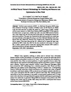
TABLE I RESULTS FOR MLP NEURAL NETWORKS
E. Mackey–Glass Data Set In experiments, the neural network was used to predict points of the time series that result of the Mackey–Glass equation integration [10], given by (17) It is a time series with chaotic behavior, recognized as a reference in the study of the learning and generalization capacity of different architectures of neural networks and neurofuzzy systems. To obtain the time series value at integer points, fourthorder Runge–Kutta method was applied to generate 1000 data points. The time step used assumed the values , and for . The neural network training was done using 500 data points to ), using 250 data points to validation ( ( to ), by giving four inputs ( and ), and . The neural network we attempted to predict the output were tested with another 250 data points ( to ). In the classification problems, the data for training and testing the artificial neural network were divided as follows: 50% of the patterns from each class were assigned randomly to the training set, 25% were assigned to the validation set, and 25% were reserved to test the network, as suggested by [21, Proben1]. All network units implemented the hyperbolic tangent activation function. The patterns were normalized to the range [ 1, 1], the processing units were implemented by hyperbolic tangent activation function. V. RESULTS AND DISCUSSION Simulated annealing, tabu search, and the proposed methodology were implemented. A. MLP Experiments In experiments, for each topology, ten runs were performed with 30 distinct random weight initializations. Table I presents the training of a fully connected MLP neural network by using a gradient descent with momentum backpropagation. The learning rate was set to 0.001, and the momentum term to 0.7. The parameters evaluated were 1) mean classification error of test set and 2) SEP. The best performance of MLP in the artificial nose data set was the topology using ten hidden units (which contains 90 connections), a mean classification error of 6.31%. In the iris
data set, the best results was obtained by the topology with five hidden units (which contains 35 connections), a mean classification error of 6.84%. In the thyroid data set, the smallest mean classification error (7.38%) was obtained by the topology with ten hidden units (using 240 unit connections). The full connected MLP presented the best performance in the diabetes data set using ten hidden units (which contained 72 connections), a mean classification error of 27, 08%. In the prediction problem, the Mackey–Glass data set, the best performance of the MLP was found in topology using four hidden units (which contains 20 connections), a squared error percentage of 1.43. Therefore, it becomes important to optimize the network topologies, in order to verify if MLP networks can obtain better performances when the architecture is defined by an optimization method. B. Optimization Methodologies Experiments For SA, TS, and the proposed methodology, the maximal topology in the artificial nose data set contains six input units, ten hidden units, and three output units ( and ; the maximum number of connections is equal to 90). In the iris data set, the maximal topology contains and . For the thyroid data set, the maximal topology contains and . In the diabetes data set, the maximal topology and . In contains the Mackey–Glass experiments, the maximal topology contains and . In the experiments with simulated annealing, the representation of solutions, the cost function, and the generation mechanism for new solutions were the same as explained in Section III. was set to The probability of inverting the connectivity bits was set to 1, and the tempera20%. The initial temperature was set to 0.9. The temperature was decreased at ture factor each ten iterations , and the maximum number of iterations was set to 1000. The performance of simulated annealing is impacted by the choice of its parameters, but there are no rules for adjusting the configuration to produce better results. Thus, the configuration used in this paper, which was chosen after some preliminary experiments, may not have been optimal for the problem. A more rigorous parameter exploration may have generated better
LUDERMIR et al.: AN OPTIMIZATION METHODOLOGY FOR NEURAL NETWORK WEIGHTS AND ARCHITECTURES
results, but this paper does not intend to present an exhaustive exploration of the adjustable parameters, which would be very time consuming. This paper aims to show that good results have been achieved by simulated annealing for the optimization problem, despite its difficulty for parameter adjustment. In the experiments with tabu search, the representation of solutions, the cost function, and the generation mechanism for new solutions are the same as used in the SA implementation, as well as the probability of inverting the connectivity bits. In each iteration, the generation mechanism produces 20 distinct new solutions, and the algorithm chooses the best one (in terms of the cost function) which is not in the tabu list. The tabu list stores the ten most recently visited solutions. Since the connection weights are real numbers, the likelihood of finding solutions that are identical is extremely small. Therefore, a proximity criterion is used to relax the strict comparison of weights, as implemented by Sexton et al. for the training of feedforward neural networks [11]. According to this criterion, a new solution is considered equal to one of the tabu solutions in the list if each connectivity bit in the new solution is identical to the corresponding connectivity bit in the tabu solution and if of the each connection weight in the new solution is within corresponding connection weight in the tabu solution, where the parameter is a real number. In this paper, is set to 0.01. As in the SA experiments, there are no rules for adjusting the TS parameters to produce better results, and the configuration used in this paper was chosen after some preliminary experiments and may not have been optimal for the problem. Again, this paper aims to show that good results can be achieved by TS for the problem, despite its difficulty for parameter adjustment. The maximum number of iterations allowed for TS is 100. This number is less than the maximum number of iterations in the SA experiments (1000), since each iteration of TS evaluates a set of neighbors, instead of only one neighbor solution. For this reason, TS needs, in general, fewer iterations to converge than SA. The proposed methodology was implemented using the same parameters adopted in the SA experiments, but the maximum number of iterations was set to 100, since the method evaluates a set of 20 new solutions at each iteration, as done by TS. In order to improve the generalization performance of the networks, the topologies given as solutions by optimization methods were trained with the backpropagation with momentum algorithm, in a hybrid training approach, as discussed before. The parameters of the backpropagation algorithm for fine-tuning were: learning rate was set to 0.001 and the momentum term to 0.7. For each initial topology, ten distinct random weight initializations were used, and the initial weights were taken from a uniform distribution between 1.0 and 1.0. The results for SA, TS, and the proposed methodology are presented in Table II. It can be seen, for all data sets, that the networks obtain low classification error when compared to those obtained by MLP networks without topology optimization (Table I) and the mean number of connections is much lower than the maximum number allowed. In all data sets, the best optimization performance was obtained by the proposed methodology. For the artificial nose data set, the classification error was around 1.42% (the full connected MLP obtained a
1457
TABLE II RESULTS FOR THE OPTIMIZATION APPROACHES
classification error of 6.30%) and the mean number of connections 29.10 (the maximum number allowed was 90). In the iris data set, the best classification error was of 4.61% (6.84% in a full connected MLP) and the mean number of connections 7.73 (maximum of 35). In the thyroid data set, the mean classification error was 7.33% (7.38% in a fully connected MLP) and the mean number of connections 71.54 of 240 allowed in a fully connected network. For the diabetes data set, the mean classification error was of 25.87% (the fully connected MLP obtained an error of 27.08%) using mean connection number of 25.50 (100 connections allowed). For the prediction problem, the Mackey–Glass data set, the obtained squared error percentage was 0.68 (1.43 in a full connected neural network) using a mean of 8.56 connections of 20 allowed in a fully connected MLP. It can be seen that the performances of TS and SA are similar, for all data sets. A paired-differences test with 95% confidence level [24] was applied in order to confirm the statistical significance of these conclusions. The superiority of the results obtained by TS, in most of the cases, can be explained in the following way: at each iteration, TS evaluates 20 new solutions; therefore it has a greater chance to find better solutions in the search space. The SA method evaluates a single new solution at each iteration; thus it needs more iterations to find good solutions. The maximum number of iterations for SA was 1000, but this quantity may have not been enough for allowing a satisfactory exploration in the search space. In contrast with SA, TS used a maximum of 100 iterations in experiments. For the proposed methodology, the test has concluded that the classification error was statistically lower than the iris and artificial nose data sets and statistically equivalent to that obtained by the other methods in the remainder data sets. The mean number of connections for the proposed methodology was lower than all remaining approaches, for all data sets. It can be seen
1458
IEEE TRANSACTIONS ON NEURAL NETWORKS, VOL. 17, NO. 6, NOVEMBER 2006
that the proposed methodology is able to perform a better exploration in the topology search space due to the combination of the advantages of SA and TS, in order to generate MLP networks with small number of connections and high classification performance. All the approaches implemented in this paper are able to eliminate input units in MLP topologies. Therefore, it is important to verify which input features are discarded and which are more relevant in the neural networks results. In experiments, the proposed methodology performed a better exploration in the architecture search space than the remaining approaches, generating a larger number of topologies, which do not need all these inputs. The inputs with the highest usage frequency have the highest importance in the classification or prediction task (e.g., in the artificial nose data set, the first sensor certainly has obtained the most significant differences in the responses for the three vintages of wine). This information can be used in real applications to reduce the database complexity and improve the performance of the classifier. VI. FINAL REMARKS This paper has shown that the combination of simulated annealing and tabu search in the proposed methodology can be used successfully for simultaneous optimization of MLP network topology and weights. Both the architecture and the weights of an MLP network were represented in the same solution, which is considered as a point in the search space. In this way, the methodology searches for the global minimum, which represents an MLP network with low complexity and good performance. Considering the data sets used in this paper, the methodology was able to generate automatically MLP topologies with many fewer connections than the maximum number allowed. The results also generate interesting conclusions about the importance of each input feature in the classification and prediction task. The proposed methodology was originally not designed to deal with different number of hidden layers but it does work with different numbers of hidden layers. Some experiments were made with more than one hidden layer. In any case, a decision needs to be made about the size of the initial topology. So in the experiments made in this paper, the initial topologies have only one hidden layer with all possible feedforward connections. As future work, some regularization methods, such as weight decay and weight elimination [25], could be used to improve the cost function. REFERENCES [1] D. E. Rumelhart, G. E. Hinton, and R. J. Williams, “Learning internal representations by error propagation,” in Parallel Distributed Processing, D. E. Rumelhart and J. L. McClelland, Eds. Cambridge, MA: MIT Press, 1986, vol. 1, pp. 318–362. [2] S. Kirkpatrick, C. D. Gellat, Jr., and M. P. Vecchi, “Optimization by simulated annealing,” Science, vol. 220, pp. 671–680, 1983. [3] F. Glover, “Future paths for integer programming and links to artificial intelligence,” Comput. Oper. Res., vol. 13, pp. 533–549, 1986. [4] J. H. Holland, Adaptation in Natural and Artificial Systems. Ann Arbor, MI: Univ. Michigan Press, 1975. [5] X. Yao, “Evolving artificial neural networks,” Proc. IEEE, vol. 87, no. 9, pp. 1423–1447, Sep. 1999.
[6] J. E. G. de Souza, B. B. Neto, F. L. dos Santos, C. P. de Melo, M. S. Santos, and T. B. Ludermir, “Polypyrrole based aroma sensor,” Synth. Metals, vol. 102, pp. 1296–1299, 1999. [7] C. L. Blake and C. J. Merz, UCI Repository of Machine Learning Databases. Irvine, CA: Dept. Inf. Comput. Sci., Univ. California, 1998. [8] E. Anderson, “The irises of the Gaspé peninsula,” Bull. Amer. Iris Soc., vol. 59, pp. 2–5, 1953. [9] J. Quinlan, “Simplifying decision trees,” Int. J. Man–Machine Studies, vol. 27, pp. 221–234, 1987. [10] M. C. Mackey and L. Glass, “Oscillation and chaos in physiological control systems,” Science, vol. 197, pp. 287–289, 1977. [11] R. S. Sexton, B. Alidaee, R. E. Dorsey, and J. D. Johnson, “Global optimization for artificial neural networks: A tabu search application,” Eur. J. Oper. Res., vol. 106, no. 2–3, pp. 570–584, 1998. [12] R. S. Sexton, R. E. Dorsey, and J. D. Johnson, “Optimization of neural networks: A comparative analysis of the genetic algorithm and simulated annealing,” Eur. J. Oper. Res., vol. 114, pp. 589–601, 1999. [13] J. Tsai, J. Chou, and T. Liu, “Tuning the structure and parameters of a neural network by using hybrid Taguchi-genetic algorithm,” IEEE Trans. Neural Netw., vol. 17, no. 1, pp. 69–80, Jan. 2006. [14] P. P. Palmes, T. Hayasaka, and S. Usui, “Mutation-based genetic neural network,” IEEE Trans. Neural Netw., vol. 16, no. 3, pp. 587–600, May 2005. [15] S. Chalup and F. Maire, “A study on hill climbing algorithms for neural network training,” in Proc. 1999 Congr. Evol. Comput., 1999, vol. 3, pp. 2014–2021. [16] N. K. Treadgold and T. D. Gedeon, “Simulated annealing and weight decay in adaptive learning: The SARPROP algorithm’’,” IEEE Trans. Neural Netw., vol. 9, no. 4, pp. 662–668, Jul. 1998. [17] K. D. Boese and A. B. Kahng, “Simulated annealing of neural networks: The ‘cooling’ strategy reconsidered,” in Proc. IEEE Int. Symp. Circuits Syst., 1993, pp. 2572–2575. [18] Q. Ying-Jian, L. Si-Wei, L. Jian-Yu, and T. Hong, “Training MLP via the deterministic anneliang EM algorithm,” Int. Conf. Machine Learn. Cybern., vol. 3, pp. 1409–1413, 2002. [19] D. Karaboga and A. Kalinli, “Training recurrent neural networks for dynamic system identification using parallel tabu search algorithm,” in 12th IEEE Int. Symp. Intell. Contr., Istanbul, Turkey, 1997, pp. 113–118. [20] R. Battiti and G. Tecchiolli, “Training neural nets with the reactive tabu search,” IEEE Trans. Neural Netw., vol. 6, no. 5, pp. 1185–1200, Sep. 1995. [21] L. Prechelt, Proben1—A set of neural network benchmark problems and benchmarking rules Fakultät für Informatik, Universität Karlsruhe, Karlsruhe, Germany, Tech. Rep. 21/94, Sep. 1994. [22] A. Yamazaki and T. B. Ludermir, “Neural network training with global optimization techniques,” Int. J. Intell. Syst., vol. 13, no. 2, pp. 77–86, 2003. [23] A. Yamazaki, T. B. Ludermir, and M. C. P. de Souto, “Classification of vintages of wine by an artificial nose using time delay neural networks,” Electron. Lett., vol. 37, no. 24, pp. 1466–1467, Nov. 22, 2001. [24] T. M. Mitchell, “Evaluating hypotheses,” in Machine Learning. New York: WCB/McGraw-Hill, 1997, pp. 128–153. [25] A. S. Weigend, D. E. Rumelhart, D. E. , and B. A. Huberman, “Generalization by weight-elimination with application to forecasting,” in Advances in Neural Information Processing Systems 3, R. P. Lippmann, J. Moody, and D. S. Touretzky, Eds. San Mateo, CA: Morgan Kaufmann, 1991, pp. 875–882.
Teresa B. Ludermir received the Ph.D. degree in artificial neural networks from Imperial College, University of London, London, U.K., in 1990. From 1991 to 1992, she was a Lecturer with Kings College, London, U.K. She joined the Center of Informatics, Federal University of Pernambuco, Pernambuco, Brazil, in 1992, where she is currently a Professor and Head of the Computational Intelligence Group. She has published more than 150 articles in scientific journals and conferences and two books on neural networks. Her research interests include weightless neural networks, hybrid neural systems, and applications of neural networks. Dr. Ludermir is an Editor-in-Chief of the International Journal of Computation Intelligence and Applications. She organized two Brazilian Symposia on Neural Networks.
LUDERMIR et al.: AN OPTIMIZATION METHODOLOGY FOR NEURAL NETWORK WEIGHTS AND ARCHITECTURES
Akio Yamazaki received the M.S. and Ph.D. degrees in computer science from the Federal University of Pernambuco, Pernambuco, Brazil, in 2001 and 2004, respectively. His research interest is in artificial neural networks.
1459
Cleber Zanchettin received the B.S. degree from West Santa Catarina University, Santa Catarina, Brazil, and the M.S. degree from the Federal University of Pernambuco, Pernambuco, Brazil, both in computer science. He is currently working towards the Ph.D. degree (artificial neural network optimization) at Federal University of Pernambuco. He is a Technical Reviewer and has published papers in the areas of pattern recognition, artificial neural networks, and intelligent systems.