Anchor Modeling – Agile Information Modeling in Evolving Data

Anchor Modeling – Agile Information Modeling in Evolving Data Environments L. R¨onnb¨ack Resight, Kungsgatan 66, 101 30 Stockholm, Sweden

O. Regardt Teracom, Kakn¨ astornet, 102 52 Stockholm, Sweden

M. Bergholtz, P. Johannesson, P. Wohed DSV, Stockholm University, Forum 100, 164 40 Kista, Sweden

Abstract Maintaining and evolving data warehouses is a complex, error prone, and time consuming activity. The main reason for this state of affairs is that the environment of a data warehouse is in constant change, while the warehouse itself needs to provide a stable and consistent interface to information spanning extended periods of time. In this article, we propose an agile information modeling technique, called Anchor Modeling, that offers non-destructive extensibility mechanisms, thereby enabling robust and flexible management of changes. A key benefit of Anchor Modeling is that changes in a data warehouse environment only require extensions, not modifications, to the data warehouse. Such changes, therefore, do not require immediate modifications of existing applications, since all previous versions of the database schema are available as subsets of the current schema. Anchor Modeling decouples the evolution and application of a database, which when building a data warehouse enables shrinking of the initial project scope. While data models were previously made to capture every facet of a domain in a single phase of development, in Anchor Modeling fragments can be iteratively modeled and applied. We provide a formal and technology independent definition of anchor models and show how anchor models can be realized as relational databases together with examples of schema evolution. We also investigate performance through a number of lab experiments, which indicate that under certain conditions anchor databases perform substantially better than databases constructed using traditional modeling techniques. Keywords: Anchor Modeling, database modeling, normalization, 6NF, data warehousing, agile development, temporal databases, table elimination

1. Introduction Maintaining and evolving data warehouses is a complex, error prone, and time consuming activity. The main reason for this state of affairs is that the environment of a data warehouse is in constant change, while the warehouse itself needs to provide a stable and consistent interface to information spanning extended periods of time. Sources that deliver data to the warehouse change continuously over time and sometimes dramatically. The information retrieval needs, such as analytical and reporting needs, also change. In order

Email addresses: [email protected] (L. R¨ onnb¨ ack), [email protected] (O. Regardt), [email protected] (M. Bergholtz), [email protected] (P. Johannesson), [email protected] (P. Wohed) Preprint submitted to DKE

October 5, 2010

to address these challenges, data models of warehouses have to be modular, flexible, and track changes in the handled information [18]. However, many existing warehouses suffer from having a model that does not fulfil these requirements. One third of implemented warehouses have at some point, usually within the first four years, changed their architecture, and less than a third quotes their warehouses as being a success [33]. Anchor Modeling is a graphic data modeling technique including a number of modeling patterns. These patterns are embodied in a set of novel constructs capturing aspects such as historization and fixed sets of entities, introduced to support data designers. In addition, Anchor Modeling enables robust and flexible representation of changes. All changes are done in the form of extensions, which make different versions of a model continuously available as subsets of the latest model [2]. This enables effortless cross-version querying [10]. It is also a key benefit in data warehouse environments, as applications remain unaffected by the evolution of the data model [27]. Furthermore, evolution through extensions (instead of modifications) results in modularity which makes it possible to decompose data models into small, stable and manageable components. This modularity is of great value in agile development where short iterations are required. It is simple to first construct a partial model with a small number of agreed upon business terms and later on seamlessly extended it to a complete model. This way of working can improve on the current state in data warehouse design, where close to half of current projects are either behind schedule or over budget [33], partly due to having a too large initial project scope. Furthermore, Using Anchor Modeling results in data models in which only small changes are needed when large changes occur in the environment. Changes such as adding or switching a source system or analytical tool, which are typical data warehouse scenarios, are thus easily reflected in an Anchor Model. The reduced redesign extends the longevity of a data warehouse, shortens the implementation time, and simplifies the maintenance [32]. Similarly to Kimball’s data warehouse approach [17], Anchor Modeling is heavily inspired from practice. It has been used in the insurance, logistics and retail domains, within projects spanning from departmental to enterprise wide data warehouses development. Even though the origin of Anchor Modeling were requirements found in data warehouse environments, the technique is a generic modeling approach also suitable for other types of systems. An anchor model that is realized as a relational database schema will have a high degree of normalization, provide reuse of data, offer the ability to store historical data, as well as have the benefits which Anchor Modeling brings into a data warehouse. The relationship between anchor modeling and traditional conceptual modeling techniques for relational databases, such as ER, EER, UML, and ORM, is described in Section 10. The work presented here is a continuation and extension of the results reported in [24]. The work from [24] is extended with a technique independent formalization of Anchor Modeling, translation into relational database schemas, schema evolution examples, and results from performance tests. The article is organized as follows. Section 2 defines the basic notions of Anchor Modeling in a technology independent way and proposes a naming convention, Section 3 introduces a running example, Section 4 suggests a number of Anchor Modeling guidelines, and Section 5 show how an anchor model can be realised as a relational database. In Section 6 schema evolution examples are given. Physical database implementation is described in Section 7 and Section 8 investigates such implementations with respect to performance and introduces a number of conditions that influence it. In Section 9 advantages of Anchor Modeling are discussed, Section 10 contrasts Anchor Modeling to alternative approaches in the literature, and Section 11 concludes the article and suggests directions for further research. 2. Basic Notions of Anchor Modeling In this section, we introduce the basic notions of Anchor Modeling by first explaining them informally and then giving formal definitions. The basic building blocks in Anchor Modeling are anchors, knots, attributes, and ties. A meta model for the basic notions of Anchor Modeling is given in Figure 1. Definition 1 (Identities). Let I be an infinite set of symbols, which are used as identities. Definition 2 (Data type). Let D be a data type. The domain of D is a set of data values. Definition 3 (Time type). Let T be a time type. The domain of T is a set of time values. 2

ANCHOR

1 1

1 1

type 1..*

ATTRIBUTE

0..*

domain

0..*

0..* KNOT ROLE

0..* time range

ANCHOR ROLE

1

KNOTTED STATIC KNOTTED HISTORIZED ATTRIBUTE ATTRIBUTE

0..*

1 consists_of

type

KNOTTED ATTRIBUTE

HISTORIZED ATTRIBUTE

TIE

2..*

range 0..*

range

0..*

KNOT 1

range

0..* STATIC ATTRIBUTE

1

range

DATA TYPE

consists_of KNOTTED TIE 1..* 1

KNOTTED HISTORIZED TIE

KNOTTED STATIC TIE

STATIC TIE

0..*

0..* time range 1 TIME TYPE 1 1 time range 1

HISTORIZED TIE

time range

Figure 1: A meta model for Anchor Modeling expressed in UML class diagram notation. 2.1. Anchors An anchor represents a set of entities, such as a set of actors or events. Figure 2a shows the graphical representation of an anchor. Definition 4 (Anchor). An anchor A is a string. An extension of an anchor is a subset of I. An example of an anchor is AC Actor with an example extension {#4711, #4712, #4713}. 2.2. Knots A knot is used to represent a fixed, typically small, set of entities that do not change over time. While anchors are used to represent arbitrary entities, knots are used to manage properties that are shared by many instances of some anchor. A typical example of a knot is GEN Gender, see Figure 2d, which includes two values, ‘Male’ and ‘Female’. This property, gender, is shared by many instances of the AC Actor anchor, thus using a knot minimizes redundancy. Rather than repeating the strings a single bit per instance is sufficient. Definition 5 (Knot). A knot K is a string. A knot has a domain, which is I. A knot has a range, which is a data type D. An extension of a knot K with range D is a bijective relation over I × D. An example of a knot is GEN Gender with domain I and range string. An example extension is {h#0, ‘Male’i, h#1, ‘Female’i}. 2.3. Attributes Attributes are used to represent properties of anchors. We distinguish between four kinds of attributes: static, historized, knotted static, and knotted historized, see Figure 2. A static attribute is used to represent properties of entities (anchors), where it is not needed to keep the history of changes to the attribute values. An example of a static attribute is birthday. A historized attribute is used when changes of the attribute values need to be recorded. An example of a historized attribute is weight. A knotted static attribute is used to represent relationships between anchors and knots, i.e. to relate an anchor to properties that can take on only a fixed, typically small, number of values. Finally a knotted historized attribute is used when the relationship with a knot value is not stable but may change over time. Definition 6 (Static Attribute). A static attribute BS is a string. A static attribute BS has an anchor A for domain and a data type D for range. An extension of a static attribute BS is a relation over I × D. An example of a static attribute is ST LOC Stage Location with domain ST Stage and range string. An example extension is {h#55, ‘Maiden Lane’i, h#56, ‘Drury Lane’i}. 3

ST_NAM_Stage_Name

AC_Actor ST_LOC_Stage_Location

(a)

(b) GEN_Gender

GEN_Gender

(d)

AC_GEN_Actor_Gender

(e)

(c) AC_PLV_Actor_ProfessionalLevel

PLV_ProfessionalLevel

(f)

Figure 2: An anchor (a) is shown as a filled square and a knot (d) as an outlined square with slightly rounded corners. A static attribute (b) and a knotted static attribute (e) are shown as outlined circles. A historized attribute (c) and a knotted historized attribute (f) are shown as circles with double outlines. Knotted attributes reference a knot. Definition 7 (Historized Attribute). A historized attribute BH is a string. A historized attribute BH has an anchor A for domain, a data type D for range, and a time type T as time range. An extension of a historized attribute BH is a relation over I × D × T. An example of a historized attribute is ST NAM Stage Name with domain ST Stage, range string, and time range date. An example extension is {h#55, ‘The Globe Theatre’, 1599-01-01i, h#55, ‘Shakespeare’s Globe’, 1997-01-01i, h#56, ‘Cockpit’, 1609-01-01i}. Definition 8 (Knotted Static Attribute). A knotted static attribute BKS is a string. A knotted static attribute BKS has an anchor A for domain and a knot K for range. An extension of a knotted static attribute BKS is a relation over I × I. An example of a knotted static attribute is AC GEN Actor Gender with domain AC Actor and range GEN Gender. An example extension is {h#4711, #0i, h#4712, #1i}. Definition 9 (Knotted Historized Attribute). A knotted historized attribute BKH is a string. A knotted historized attribute BKH has an anchor A for domain, a knot K for range, and a time type T for time range. An extension of a knotted historized attribute BKH is a relation over I × I × T. An example of a knotted historized attribute is AC PLV Actor ProfessionalLevel with domain AC Actor, range PLV ProfessionalLevel, and time range date. An example extension is {h#4711, #4, 1999-04-21i, h#4711, #5, 2003-08-21i, h#4712, #3, 1999-04-21i}. 2.4. Ties A tie represents an association between two or more anchor entities and optional knot entities. Similarly to attributes, ties come in four variants, static, historized, knotted static, and knotted historized. See Figure 3. As the same entity may appear more than once in a tie, occurrences need to be qualified using the concept of roles. Definition 10 (Anchor Role). An anchor role is a string. Every anchor role has a type, which is an anchor. Definition 11 (Knot Role). A knot role is a string. Every knot role has a type, which is a knot. An example of an anchor role is atLocation, with type ST Stage, and an example of a knot role is having, with type PAT ParentalType. Definition 12 (Static Tie). A static tie TS is a set of at least two anchor roles. An instance tS of a static tie TS = {R1 , . . . , Rn } is a set of pairs hRi , vi i, i = 1, . . . , n, where Ri is an anchor role, vi ∈ I and n ≥ 2. An extension of a static tie TS is a set of instances of TS . 4

PE_wasHeld_ST_atLocation

ST_atLocation_PR_isPlaying

(a)

(b)

RAT_Rating AC_parent_AC_child_PAT_having

PAT_ParentalType

AC_part_PR_in_RAT_got

(c)

(d)

Figure 3: A static tie (a) and a knotted static tie (c) are shown as filled diamonds. A historized tie (b) and a knotted historized tie (d) are shown as filled diamonds with an extra outline. Knotted ties reference at least one knot. Identifiers of the ties are marked with black circles. An example of a static tie is PE wasHeld ST atLocation = {wasHeld, atLocation}, where the type of wasHeld is PE Performance and the type of atLocation is ST Stage. An example extension is {{hwasHeld, #911i, hatLocation, #55i}, {hwasHeld, #912i, hatLocation, #55i}, {hwasHeld, #913i, hatLocation, #56i}}. Definition 13 (Historized Tie). A historized tie TH is a set of at least two anchor roles and a time type T. An instance tH of a historized tie TH = {R1 , . . . , Rn , T} is a set of pairs hRi , vi i, i = 1, . . . , n and a time point p, where Ri is an anchor role, vi ∈ I, p ∈ T, and n ≥ 2. An extension of a historized tie TH is a set of instances of TH . An example of a historized tie is ST atLocation PR isPlaying = {atLocation, isPlaying, date}, where the type of atLocation is ST Stage and the type of isPlaying is PR Program. An example extension is {{hatLocation, #55i, hisPlaying, #17i, 2003-12-13}, {hatLocation, #55i, hisPlaying, #23i, 2004-04-01}, {hatLocation, #56i, hisPlaying, #17i, 2003-12-31}}. Definition 14 (Knotted Static Tie). A knotted static tie TKS is a set of at least two anchor roles and one or more knot roles. An instance tKS of a static tie TKS = {R1 , . . . , Rn , S1 , . . . , Sm } is a set of pairs hRi , vi i, i = 1, . . . , n and hSj , wj i, j = 1, . . . , m, where Ri is an anchor role, Sj is a knot role, vi ∈ I, wj ∈ I, n ≥ 2, and m ≥ 1. An extension of a knotted static tie TKS is a set of instances of TKS . Definition 15 (Knotted Historized Tie). A knotted historized tie TKH is a set of at least two anchor roles, one or more knot roles and a time type T. An instance tKH of a historized tie TKH = {R1 , . . . , Rn , S1 , . . . , Sm , T} is a set of pairs hRi , vi i, i = 1, . . . , n, hSj , wj i, j = 1, . . . , m, and a time point p, where Ri is an anchor role, Sj is a knot role, vi ∈ I, wj ∈ I, p ∈ T, n ≥ 2, and m ≥ 1. An extension of a knotted historized tie TKH is a set of instances of TKH . Definition 16 (Identifier). Let T be a (static, historized, knotted, or knotted historized) tie. An identifier for T is a subset of T containing at least one anchor role. Furthermore, if T is a historized or knotted historized tie, where T is the time type in T , every identifier for T must contain T. An identifier is similar to a key in relational databases, i.e. it should be a minimal set of roles that uniquely identifies instances of a tie. The circles on the tie edges in Figure 3 indicate whether the connected entity is part of the identifier (filled black) or not (filled white). Definition 17 (Anchor Schema). An anchor schema is a 13-tuple hA, K, BS , BH , BKS , BKH , RA , RK , TS , TH , TKS , TKH , Ii, where A is a set of anchors, K is a set of knots, BS is a set of static attributes, BH is a set of historized attributes, BKS is a set of knotted static attributes, BKH is a set of knotted historized attributes, RA is a set of anchor roles, RK is a set of knot roles, TS is a set of static ties, TH is a set of historized ties, 5

TKS is a set of knotted static ties, TKH is a set of knotted historized ties, and I is a set of identifiers. The following must hold for an anchor schema: (i) for every attribute B ∈ BS ∪ BH ∪ BKS ∪ BKH , domain(B) ∈ A (ii) for every attribute B ∈ BKS ∪ BKH , range(B) ∈ K (iii) for every anchor role RA ∈ RA , type(RA ) ∈ A (iv) for every knot role RK ∈ RK , type(RK ) ∈ K (v) for every tie T ∈ TS ∪ TH ∪ TKS ∪ TKH , T ⊆ RA ∪ RK Definition 18 (Anchor Model). Let A = hA, K, BS , BH , BKS , BKH , RA , RK , TS , TH , TKS , TKH , Ii be an anchor schema. An anchor model for A is a quadruple hextA , extK , extB , extT i, where extA is a function from anchors to extensions of anchors, extK is a function from knots to extensions of knots, extB is a function from attributes to extensions of attributes, and extT is a function from ties to extensions of ties. Let proji be the ith projection map. An anchor model must fulfil the following conditions: (i) for every attribute B ∈ BS ∪ BH ∪ BKS ∪ BKH , proj1 (extB (B)) ⊆ extA (domain(B)) (ii) for every attribute B ∈ BKS ∪ BKH , proj2 (extB (B)) ⊆ proj1 (extK (range(B))) (iii) for every tie T and anchor role RA ∈ T , {v | hRA , vi ∈ extT (T )} ⊆ extA (type(RA )) (iv) for every tie T and knot role RK ∈ T , {v | hRK , vi ∈ extT (T )} ⊆ proj1 (extK (type(RK ))) (v) every extension of a tie T ∈ TS ∪ TH ∪ TKS ∪ TKH shall respect the identifiers in I, where an extension extT (T ) of a tie respects an identifier I ∈ I if and only if it holds that whenever two instances t1 and t2 of extT (T ) agree on all roles in I, and for historized ties also the time range, then t1 = t2 . 2.5. Naming Convention Entities in an anchor schema can be named in any manner, but having a naming convention outlining how names should be constructed increases understandability and simplifies working with a model. If the same convention is used consistently over many installations the induced familiarity will significantly speed up recognition of the entities and their relation to other entities. A good naming convention should fulfill a number of criteria, some of which may conflict with others. Names should be short, but long enough to be intelligible. They should be unique, but have parts in common with related entities. They should be unambiguous, without too many rules having to be introduced. Furthermore, in order to be used in many different representations, the less “exotic” characters they contain the better. We suggest a naming convention that is summarized in Figure 4. A formal definition can be found in [28]. The suggested convention uses only regular letters, numbers, and the underscore character. This ensures that the same names can be used in a variety of representations, such as in a relational database, in XML, or in a programming language. Entity

Mnemonic/pattern

Descriptor/pattern

Name

Example

Anchor Knot Attribute Role Tie

Am Km Bm

Ad Kd Bd r

Am Km Am r Am

AC Actor GEN Gender AC GEN Actor Gender wasCast PE in AC wasCast

[A-Z]{2} [A-Z]{3} [A-Z]{3}

([A-Z][a-z]*)+ ([A-Z][a-z]*)+ ([A-Z][a-z]*)+ ([a-z][A-Z]*)+

Ad Kd B m Ad B d r . . . (Km r)

Figure 4: Entity naming convention, using regular expressions to describe the syntax. The suggested naming convention uses a syntax with a few semantic rules, making it possible to derive the immediate relations of an entity given its name. It also defines names for the constituents of an entity. The syntax uses three primitives: mnemonics, descriptors and roles. Names are then constructed using combinations of these primitives. The manner in which these are combined is determined by the result of letting semantic rules operate on the structure of the model. Anchor and knot mnemonics are unique in the model, while attribute mnemonics need only be unique in the set of attributes referencing the same anchor. The names of ties are built from the mnemonics of adjoined anchors and knots together with the roles they play in the relationship. Names of constituents are semantically connected to the encapsulating or referenced entity. Names of identities are mnemonics suffixed with ‘ID’, and in ties also with the role they take. Names of time ranges have ‘ValidFrom’ as a suffix. Data ranges share names with their encapsulating entity. 6

3. Running Example The scenario in this example is based on a business arranging stage performances. It is an extension of the example discussed in [16]. An anchor schema for this example is shown in Figure 5. The business entities are the stages on which performances are held, programs defining the actual performance, i.e. what is performed on the stage, and actors who carry out the performances. Stages have two attributes, a name and a location. The name may change over time, but not the location. Programs just have a name, which describes the act. If a program changes name it is considered to be a different act. Actors have a name, but since this may be a pseudonym it could change over time. They also have a gender, which we assume does not change. The business also keeps track of an actor’s professional level, which changes over time as the actor gains experience. Actors get a rating for each program they have performed. If they perform consistently better or worse, the rating changes to reflect this. Stages are playing exactly one program at any given time and they change program every now and then. To simplify casting, the parenthood between actors is needed so that it is possible to determine if an actor is the mother or father of another actor. A performance is an event bound in space and time that involves a stage on which a certain program is performed by one or more actors. It is uniquely identified by when and where it was held. The managers of the business also need to know how large the audience was at every performance and the total revenue gained from it. PE_REV_Performance_Revenue ST_NAM_Stage_Name

PE_DAT_Performance_Date

PE_wasHeld_ST_atLocation

PE_AUD_Performance_Audience ST_Stage

ST_LOC_Stage_Location

PE_Performance

PE_in_AC_wasCast GEN_Gender

ST_atLocation_PR_isPlaying PE_at_PR_wasPlayed

AC_GEN_Actor_Gender RAT_Rating

PR_Program

AC_Actor AC_NAM_Actor_Name PR_NAM_Program_Name AC_part_PR_in_RAT_got AC_parent_AC_child_PAT_having AC_PLV_Actor_ProfessionalLevel

PLV_ProfessionalLevel

PAT_ParentalType

Figure 5: A graphically represented anchor schema illustrating different modeling concepts. Four anchors PE Performance, ST Stage, PR Program and AC Actor capture the present entities. Attributes such as PR NAM Program Name and PE DAT Performance Date capture properties of those entities. Some attributes, e.g. AC NAM Actor Name and ST NAM Stage Name are historized, to capture the fact that they are subject to changes. The fact that an actor has a gender, which is one of two possible values, is captured through the knot GEN Gender and a knotted attribute called AC GEN Actor Gender. Similarly, since the business also keeps tracks of the professional level of actors, the knot PLV ProfessionalLevel and the knotted attribute AC PLV Actor ProfessionalLevel are introduced, which in addition is historized to capture attribute value changes. The relationships between the anchors are captured through ties. In the example the following ties are introduced: PE in AC wasCast, PE wasHeld ST atLocation, PE at PR wasPlayed, ST atLocation PR isPlaying, AC part PR in RAT got, and AC parent AC child PAT having to capture the existing binary relationships. The historized tie ST atLocation PR isPlaying is used to capture the fact that stages change 7

programs. The tie AC part PR in RAT got is knotted to show that actors get ratings on the programs they are playing and historized for capturing the changes in these ratings. 4. Guidelines for Designing Anchor Models Anchor Modeling has been used in a number of industrial data warehouse projects in the insurance, logistics and retail businesses, ranging in scope from departmental to enterprise wide. Based on this experience and a number of well-known modeling problems and solutions i.e., reification of relationships [13], power types [8], update-anomalies in databases due to functional dependencies between attributes modeled within one entity in conceptual schemas [5], and modeling of temporal attributes [6, 11], valid time and transaction time [6, 15], the following guidelines have been formulated. 4.1. Modeling Core Entities and Transactions Core entities in the domain of interest should be represented as anchors in an anchor model. Properties of an entity are modeled as attributes on the corresponding anchor. Relationships between entities are modeled as ties. Properties of a relationship are modeled as knots or as attributes on the anchors related to the tie. A well-known problem in conceptual modeling is to determine whether a transaction should be modeled as a relationship or as an entity [13]. In Anchor Modeling, the question is formulated as determining whether a transaction should be modeled as an anchor or as a tie. When a transaction has some property, e.g., PE DAT Performance Date in Figure 5, it should be modeled as an anchor, otherwise it should be modeled as tie. Guideline 1: Use anchors for modeling core entities and transactions. A transaction should be modeled as a tie only if it has no properties. 4.2. Modeling Attribute Values Historized attributes are used when versioning of attribute value are of importance. A data warehouse, for instance, is not solely built to integrate data but also to keep a history of changes that have taken place. In anchor models, historized attributes take care of versioning by coupling versioning information, i.e. time of change, to an attribute value. Typical time granularity levels are date (e.g. ’YYYY-MM-DD’) and datetime (e.g. ’YYYY-MM-DD HH:MM’), which are also used in the article. A historized attribute value is considered valid until it is replaced by one with a later time. Valid time [6] is hence represented as an open interval with an explicitly specified beginning. The interval is implicitly closed when another attribute value with a later valid time is added for the same anchor instance. Guideline 2a: Use a historized attribute if versioning of attribute values are of importance, otherwise use a static attribute. A knot represents a type with a fixed set of instances that do not change over time. Conceptually a knot can be thought of as a an anchor with exactly one static attribute. In many respects, knots are similar to the concept of power types [8], which are types with a fixed and small set of instances representing categories of allowed values. In Figure 5 the anchor AC Actor gets its gender attribute via a knotted static attribute, AC GEN Actor Gender, rather than representing the actual gender value (i.e. the string ‘Male’ or ‘Female’) of an actor directly by a static attribute. The advantage of using knots is reuse, as attributes can be specified through references to a knot identifier instead of a value. The latter is undesirable because of the redundancy it introduces, i.e. long attribute values have to be repeated resulting in increased storage requirements and update anomalies. Guideline 2b: Use a knotted static attribute if attribute values represent categories or can take on only a fixed small set of values, otherwise use a static attribute. Guidelines 2a and 2b may be combined, i.e. when both attribute values represent categories and the versioning of these categories are of importance. 8

Guideline 2c: Use a knotted historized attribute if attribute values represent categories or a fixed small set of values and the versioning of these are of importance. 4.3. Modeling Relationships Static ties are used for relationships that do not change over time. For example, the actors who took part in a certain performance will never change. In contrast, a historized tie is used for relationships that change over time. For example, the program played at a specific stage will change over time. At any point in time, exactly one relationship will be valid. Guideline 3a: Use a historized tie if a relationship may change over time, otherwise use a static tie. Knotted ties are used for relationships of which the instances fall within certain categories. For example, a relationship between the anchors AC Actor and PR Program, may be categorized as ‘Good’, ‘Bad’ or ‘Mediocre’ indicating how well an actor performed in a program. These categories are then represented by instances of the knot RAT Rating. Guideline 3b: Use a knotted static tie if the instances of a relationship belong to certain categories, otherwise use a static tie. Guidelines 3a and 3b can also be combined in the case when a category of a relationship may change over time. Guideline 3c: Use a knotted historized tie if the instances of a relationship belong to certain categories and the relationship may change over time. 4.4. Modeling Large Relationships Anchor Modeling provides advantages such as the absence of null values [22] and update anomalies in anchor databases. These advantages rely on a high degree of decomposition, where attributes are modelled as entities of their own and relationships are made as small as possible. In the example in Section 3, we did not use a single tie for modeling the relationship between a performance, who participated in it, where it was held, and what was played. The reason for not using a single tie is that information about all parts of the relationship is needed before an instance can be created. To exemplify, an instance in the extension of such a tie PE in AC wasCast ST atLocation PR wasPlayed is {{hin, #911i, hwasCast, #4711i, hatLocation, #55i, hwasPlayed, #17i}}. Should the last piece of information, what was played at this performance, presently be missing, none of the other information can be recorded. By instead having three ties, as in the example, instances can be created independently of each other, and at different times. Guideline 4a: Use several smaller ties for which all roles are known, if roles may be temporarily unknown within a large relationship. The tie AC part PR in RAT got models the rating that an actor has got for playing a part in a certain program. This tie could be extended to having two different kinds of ratings: artistic performance and technical performance, both of which could be modeled as references to one and the same knot RAT Rating with the extension {h#1, ‘Bad’i, h#2, ‘Mediocre’i h#3, ‘Good’i}. The new tie AC part PR in RAT artistic RAT technical with extension {{hpart, #4711i, hin, #17i, hartistic, #2i, htechnical, #2i, 2005-03-12}, {hpart, #4711i, hin, #17i, hartistic, #3i, htechnical, #2i, 2008-08-29}}}, suffers from the modeling counterpart of update anomalies [5]. It is no longer possible to discern to which of the two ratings (artistic or technical) the historization date refers. The situation occurs in historized ties when more than one role is not in the identifier for the tie. If this situation occurs it is better to model the relationship as several ties for which those that are still historized have exactly one role outside the identifier. In the example given the tie would be decomposed into two ties AC part PR in RAT artistic and AC part PR in RAT technical, for which there can be no doubt as to what has changed between versions. Guideline 4b: Include in a (knotted) historized tie at most one role outside the identifier. 9

For a tie having one or more knot roles, it is sometimes desirable to remodel the tie such that it only contains anchor roles. This can be achieved by introducing a new anchor on which the knots appear through knotted attributes and a role for that anchor replacing the knot roles in the tie. Consider a situation in which we have a knotted historized tie of high cardinality with all anchor roles and all but one knot role in its identifier. If roles do not change synchronously, for every new version that is added only the historization part of the identifier changes and the rest will be duplicated, and if that remainder is long it leads to unnecessary duplication of data. For example, let an extension be {{hRA1 , #1i, . . . , hRAn , #ni, hRK , #21i, 2010-02-25 10:52:21}, {hRA1 , #1i, . . . , hRAn , #ni, hRK , #22i, 2010-02-25 10:52:22}}. A remodeling to a static tie is possible. The new tie has {{hRA1 , #1i, . . . , hRAn , #ni, hRA new , #538i}}, the introduced anchor has {#538}, and the introduced knotted historized attribute has {h#538, #21, 2010-02-25 10:52:21i, h#538, #22, 2010-02-25 10:52:22i} as extensions. The new model duplicates less data and makes the retrieval of the history over changes in the knotted identities (and values if joined) optional, but it also puts the values “farther away” from the tie. Whether or not to remodel will depend on the amount of duplication and how fast this duplication will occur by the speed with which new versions arrive. Guideline 4c: Replace the knot roles in a tie with an anchor role and an anchor with knotted attributes, if roles do not change synchronously within the relationship. 4.5. Modeling States A state is a time dependent condition, such that for any given time point it is either true or false. Over a period of time there may be sequential intervals in which a condition is interchangeably true or false. Since historized attributes and ties can only model the starting point of such an interval, the only way to exit a state is by the transition into a mutually exclusive state. For example, being married is a state, and if divorced there is likely to be a time of being single (in a non-married state) before the next marriage. The information that an actor was married between 1945-10-17 and 1947-08-29 cannot be captured by a single instance in an anchor model. Two instances are needed, one for when the actor entered the married state with the time point 1945-10-17 and one for when the actor entered the unmarried state with the time point 1947-08-29. In Anchor Modeling knots are used to model states of entities, attributes, and relationships. The states a specific knot is modeling should also be mutually exclusive, such that no two of them can both be true, and exhaustive, such that one of them is always true. In the most basic and common form, modeled states are of the types ‘in state’ and ‘not in state’. For instance, a knot modeling the states needed to capture marriage can have the extension {h#0, ‘Not married’i, h#1, ‘Married’i}. Of the two conditions ‘Not married’ and ‘Married’, exactly one is true at any given moment. A more advanced state model would have the form ‘in first state’, . . . , ‘in nth state’, and ‘in neither of first to nth state’. An example extension for such a knot is {h#1, ‘Red’i, h#2, ‘Green’i, h#3, ‘Blue’i, h#0, ‘Lacking color’i}. Guideline 5: Use knots to model states of entities, attributes, and relationships, for which the states represented by a knot should be mutually exclusive and exhaustive. The example in Section 3 can be extended to handle such states as when an actor resigns, when an actor stops having a professional level due to inactivity, or when a stage is not playing any program at all. For example the knot ACT Active with the extension {h#0, ‘Resigned’i, h#1, ‘Active’i} and a knotted historized attribute AC ACT Actor Active can be used to determine whether an actor is still active or not. The knot PLV ProfessionalLevel can be extended with the state ‘Expired’, to determine whether an actor’s professional level has expired or not. Finally, the knot PST PlayingStatus with the extension {h#0, ‘Stopped’i, h#1, ‘Started’i} and a knotted historized tie ST atLocation PR isPlaying PST currentStatus can be used to determine the durations with which programs are playing at the stages. Note, however, that not all attributes that change over time represent states. For example, the attribute ‘weight’, whose values may change over time, is not represented by states. Whenever a new weight is measured it simply replaces the old one and the essential difference is that there is no ‘non-weight state that can be had. This should not be confused with an unknown weight, which would result in the absence of an instance. 10

5. From Anchor Model to Relational Database An anchor schema can be automatically translated to a relational database schema through a number of transformation rules. An open source modeling tool providing such functionality is available on-line at http://www.anchormodeling.com/modeler. Here we present the intuition behind the translation. A formalization of the rules can be found in [29]. Each anchor is translated into a table containing a single column. The domain for that attribute is the set of identities I (will use the set of integers). The name of the table is the anchor and the name of the column is the abbreviation of the Anchor suffixed with ID. For example the anchor AC Actor will be translated into the table AC Actor(AC ID) where the domain for AC ID is I, see Figure 6c. A knot is translated into a binary table, in which one column contains knot values and the other one knot identities. For example, the knot GEN Gender is translated to the table GEN Gender(GEN ID, GEN Gender), see Figure 6a. GEN Gender

AC NAM Actor Name

GEN ID (PK)

GEN Gender

AC ID (PK, FK)

AC NAM Actor Name

AC NAM ValidFrom (PK)

#0 #1

‘Male’ ‘Female’

bit

string

#4711 #4711 #4712

‘Arfle B. Gloop’ ‘Voider Foobar’ ‘Nathalie Roba’

1972-08-20 1999-09-19 1989-09-21

integer

string

date

(a) knot

(b) historized attribute AC Actor

PE in AC wasCast

AC ID (PK)

PE ID in (PK, FK)

AC ID wasCast (PK, FK)

AC ID (PK, FK)

GEN ID (FK)

#4711 #4712 #4713

#911 #912 #913

#4711 #4711 #4712

#4711 #4712 #4713

#0 #1 #1

integer

integer

integer

integer

bit

(c) anchor

AC GEN Actor Gender

(d) static tie

(e) knotted static attribute

Figure 6: Example rows from the anchor AC Actor, the knot GEN Gender, the knotted static attribute AC GEN Actor Gender, the historized attribute AC NAM Actor Name, and the static tie PE in AC wasCast tables. Each attribute is translated into a distinct table containing a column for identities and a column for values. If the attribute is static the resulting table is binary. For instance, a static attribute AC NAM Actor Name will be translated into the table AC NAM Actor Name(AC ID, AC NAM Actor Name). The primary key of such tables (AC ID in this case) is a foreign key referring to the identity column of the anchor table (AC Actor.AC ID) that possesses the attribute. If the attribute is knotted, also the second column contains a foreign key. For instance, the knotted attribute AC GEN Actor Gender will be translated to the table AC GEN Actor Gender(AC ID, GEN ID), see Figure 6e, where GEN ID is a foreign key referring to the GEN Gender.GEN ID column. The tables corresponding to historized attributes contain, in addition, a third column for storing the time points at which attribute values become valid. If for instance AC NAM Actor Name is a historized attribute (as assumed in the example in Figure 6b), it will be translated to the table AC NAM Actor Name(AC ID, AC NAM Actor Name, AC NAM ValidFrom). This is done in a similar fashion for knotted historized attributes. Finally, ties are translated into tables with primary keys composed of a subset of the foreign keys that the tie refers to. For example, the static tie PE in AC wasCast is translated into the table PE in AC wasCast( PE ID in, AC ID wasCast), see Figure 6d, where both columns are part of the primary key, as well as foreign keys. AC ID wasCast refers for instance to AC Actor.AC ID. The logic for the translation of historized, knotted static, and knotted historized ties is similar to the principles of historized, knotted static, and knotted historized attributes. The complete translation of the model from Figure 5 is shown in Figure 7. Similarly 11

to the translation to relation schemas, an anchor schema can be translated to XML. An example of this is shown in [30]. Anchor Schema AC Actor PR Program ST Stage PE Performance

(AC ID∗ ) (PR ID∗ ) (ST ID∗ ) (PE ID∗ )

Knot Schema GEN Gender PLV ProfessionalLevel RAT Rating PAT ParentalType

(GEN ID∗ , GEN Gender) (PLV ID∗ , PLV ProfessionalLevel) (RAT ID∗ , RAT Rating) (PAT ID∗ , PAT ParentalType)

Attribute Schema AC GEN Actor Gender AC PLV Actor ProfessionalLevel AC NAM Actor Name PR NAM Program Name ST LOC Stage Location ST NAM Stage Name PE DAT Performance Date PE REV Performance Revenue PE AUD Performance Audience

(AC ID∗ , GEN ID) (AC ID∗ , PLV ID, AC PLV ValidFrom∗ ) (AC ID∗ , AC NAM Actor Name, AC PLV ValidFrom∗ ) (PR ID∗ , PR NAM Program Name) (ST ID∗ , ST LOC Stage Location) (ST ID∗ , ST NAM Stage Name, ST NAM ValidFrom∗ ) (PE ID∗ , PE DAT Performance Date) (PE ID∗ , PE REV Performance Revenue) (PE ID∗ , PE AUD Performance Audience)

Tie Schema AC parent AC child PAT having AC part PR in RAT got ST atLocation PR isPlaying PE in AC wasCast PE at PR wasPlayed PE wasHeld ST atLocation

(AC ID parent∗ , AC ID child ∗ , PAT ID having ∗ ) (AC ID part∗ , PR ID in∗ , RAT ID got, AC part PR in RAT got ValidFrom∗ ) (ST ID atLocation∗ , PR ID isPlaying, ST atLocation PR isPlaying ValidFrom∗ ) (PE ID in∗ , AC ID wasCast∗ ) (PE ID at∗ , PR ID wasPlayed) (PE ID wasHeld ∗ , ST ID atLocation)

Figure 7: The relational schema for the anchor schema in Figure 5 (asterisks mark primary keys).

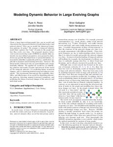
6. Schema Evolution Examples In this section the schema of the running example (Figure 5) and its corresponding implementation in a relational database will be evolved through a few examples of new requirements. One such requirement is to keep track of the durations of the programs in order to calculate the hourly revenue from a performance. This is solved by adding an attribute PR DUR Program Duration to the PR Program anchor, following Guideline 2a in Section 4 (see Figure 8). Furthermore, in order to simplify casting, which programs actors would like to play should be made available. Following Guideline 3a, this requirement is be captured by adding a static tie AC desires PR toPlay. To be able to calculate the vacancy ratio for stages, a history needs to be kept over when programs were played and when stages were vacant. The present tie ST atLocation PR isPlaying only captures the currently playing program. Following Guidelines 3c and 5 a new knotted historized tie is introduced, ST atLocation PR isPlaying PLY Playing along with the knot PLY Playing. The knot holds two values indicating whether a referring instance in the tie marks the beginning or the ending of a period in which the program was played. Usage of the old tie may be transitioned to the new one, rendering the old tie obsolete. Even though knots are assumed to be indefinitely immutable, situations may arise when the information they keep no longer fulfill its purpose. For example, say that critics introduce an new grade, “Outstanding”, for rating the acting. A solution is to add this grade as a new instance in the knot. However, to make the situation a bit more complex, critics have also decided to rename the lowest rating from “Terrible” to “Appalling”. Values in knots cannot be historized, leaving no way to express that one value has replaced 12

PE_Performance

ST_Stage

ST_atLocation_PR_isPlaying_PLY_during AC_desires_PR_toPlay PLY_Playing

(c) PR_Program

AC_Actor

(b)

AC_gained_PL_has PL_FEE_ProfessionalLevel_HourlyFee

PR_DUR_Program_Duration

(d)

(a)

PL_ProfessionalLevel

PLV_ProfessionalLevel

PL_LVL_ProfessionalLevel_Level

Figure 8: Examples of schema evolution. (a) Adding an attribute. (b) Adding a static tie. (c) Replacing a tie to gain historical capabilities. (d) Replacing a knotted attribute with a tied anchor and attributes. another in the model. If one can live with that fact, two options remain that will make the renamed rating available in the model. Either a new knot is introduced with the new names, or “Appalling” is added as an instance in the old knot. If desired, references to “Terrible” can get new instances in the tie, having references to “Appalling” and a later historization date. By only studying the model itself it is impossible to determine whether this modification is a renaming or a regrading. Another situation is when a knot starts to have properties of its own. For example, let the hourly fee for an actor depend on their professional level. Currently, the professional level is modeled as a knot, leaving no way to connect the different fees to the different levels. This can be resolved by unfolding the knot into an anchor and attributes, similar to Guideline 4c. Figure 8 shows the adding of an anchor PL ProfessionalLevel with a knotted static attribute PL LVL ProfessionalLevel Level, referring to the different professional levels. The hourly fee for each professional level is then added as a historized attribute PL FEE ProfessionaLevel HourlyFee. Finally, a historized tie AC gained PL has is added, such that the professional level for each actor can be determined. None of the schema modifications above affected the existing objects in the model. Only additions were made. Thanks to the one-to-one mapping onto the relational database schema, no existing tables will be altered by these operations. Furthermore, remaining entities will not be affected if obsolete entities are removed. As a result, evolution in an anchor schema and corresponding relational database schema can hence be done on-line and non-destructively, through extensions and by leaving every previous version as a subset of the latest schema. In situations where such a requirement is not necessary, entities may also be removed once they become obsolete. In a less normalized relational schema, the described evolution cases will involve operations altering already existing objects, which raises the complexity considerably. 7. Physical Implementation In this section an implementation of a relational database schema based on an anchor schema is discussed. We will refer to such a database schema plus its relations as an anchor database. When we discuss individual relation schemas that have their origin in anchor, tie and attribute constructs in an anchor schema we will refer to them as anchor, tie and attribute tables respectively. First the indexing of tables is discussed, followed by practices for how data should be entered into an anchor database, views and functions that 13

simplify querying, and the conditions for these to take advantage of table elimination [23] in order to gain performance. Code samples are also provided, showing how some tables, views and functions are created in Transact-SQL. 7.1. Indexes in an Anchor Database Indexes in general, and clustered indexes in particular, are used to delimit the range of a table scan or remove the need for a table scan altogether as well as removing or delimiting the need to sort searched-for-data. A clustered index is an index with a sort order equal to the physical sort order of the corresponding table on disc. In this section we will discuss what indexes on the various constructs in an anchor database will look like and motivate them from a performance point of view. Figure 10 shows how some indexes are created for different table types. Clustered unique indexes over the primary keys in an anchor database as well as unique indexes over the values in knot tables can be automatically generated given an anchor schema. 7.1.1. Indexes on Anchor and Knot Tables Since anchor tables are referenced from a number of attribute and tie tables, a unique clustered index should be created on the primary key of each anchor table. This ensures that the number of records to be scanned in queried tables will not be too large, e.g. the number of time-costly disc-accesses will be minimal. To make the treatment of indexes uniform, clustered indexes are also created for all knot tables, even if such are not always needed in theory. An additional unique index over the values in a knot table improves query performance when a condition is set on the column. Searching can then stop once a match has been found. 7.1.2. Indexes on Attribute Tables An attribute table contains a foreign key against an anchor table and optionally information on historization. A composite unique clustered index should be created on the foreign key column in ascending order together with the historization column in descending order1 . This means that on the physical media where the table data is stored, the latest version for any given identity comes first. This will ensure more efficient retrieval of data since a good query optimizer will realize that a sort operation is unnecessary. The optimizer will also utilize the created clustered indexes when joining attribute tables with their anchor table, ensuring that no sorting has to be made since both the anchor and attribute tables are already physically ordered on disc. This also means that the accesses to the storage media can be done in large sequential chunks, provided that data is not fragmented on the storage media itself. 7.1.3. Indexes on Tie Tables Tie tables contain two or more foreign keys against an anchor table, zero or more foreign keys towards knot tables, and optionally information on historization. A tie table should always have a unique clustered index over the primary key, however the order in which the columns appear can not be unambiguously determined from the identifier of the tie. An order has to be selected that fits the need best, perhaps according to what type of queries will be the most common. In some cases an additional index with another ordering of the columns may be necessary. In the running example in Section 3 the historized knotted tie AC part PR in RAT got models the current rating that an actor has got for performing a certain program, together with the time at which this rating became relevant. The unique clustered index of the corresponding tie table is composed of the foreign keys against the anchor tables in ascending order, together with the historization column in descending order. This index will ensure that we do not have to scan the entire AC Actor table for each row of the entire PR Program table in order to find the values that we are looking for. 1 Note that the indexing order of the columns is of less importance. Database engines read data in large chunks into memory and reading forwards or backwards in memory is equally effective. We do, however, in order to be consistent, use the same ordering in all of our indexes.

14

7.1.4. Partitioning of Tables In addition to indexes, access to the tables in the anchor database may be improved through partitioning. For example, if the number of actors and programs are very large and most accesses are made to the ones with the highest rating (see the historized knotted tie table above), performance can be further improved by partitioning the tie table based on the rating. Partitioning, if the database engines support it, will split the underlying data on the physical media into as many chunks as the cardinality of the knot. This allows for having frequently accessed partitions on faster discs and less data to scan during query execution. The two best candidates for partitioning in an anchor database are knot values and the time type used for historization (i.e. we assume that users tend to access certain values of knots more frequently than other values, as well as certain dates being of more or less importance). 7.2. Loading Practices When loading data into an anchor database a zero update strategy is used. This means that only insert statements are allowed and that data is always added, never updated. If there are non-persistent entities or relations in a model these have to be modeled using a knot holding the state of persistence, rather than removing rows, as discussed in Guideline 5. Delete statements are allowed only for removing erroneous data. A complete history is thereby stored for accurate information [26]. If a zero update strategy is used together with properly maintained metadata, it is always possible to find the rows that belong to a certain batch, came from a specific source system, were loaded by a particular account, or were added between some given dates. Instead of having a fault recovery system in place every time data is added, it can be prepared and used only after an error is found. Since nothing has been updated, the introduced errors are in the form of rows, and these can easily be found. Scripts can be made that allow for removal of erroneous rows, regardless of when they were added. Data will never change once it is in place, thereby guaranteeing its integrity. Avoiding updates gives an advantage in terms of performance, due to their higher cost compared to insert statements. By not doing updates there is also no row locking, a fact that lessens the impact on read performance when writing is done in the database. 7.3. Views and Functions Due to the large number of tables and the handling of historical data, an abstraction layer in the form of views and functions is added to simplify querying in an anchor database. It de-normalizes the anchor database and retrieves data from a given temporal perspective. There are three different types of views and functions introduced for each anchor table, corresponding to the most common queries: latest view, point-in-time function, and interval function [35, 26]. These are based on an abstract complete view. Views and functions for tie tables are created in a way analogous to those for anchor tables. See the right side of Figure 10 for a couple of examples of these views and functions. Note that these views and functions can be automatically generated, with the exception of the natural key view, as its composition is unknown to the schema. 7.3.1. Complete View The complete view of an anchor table is a de-normalization of it and its associated attribute tables. It is constructed by left outer joining the anchor table with all its associated attribute tables. 7.3.2. Latest View The latest view of an anchor table is a view based on the complete view, where only the latest values for historized attributes are included. A sub-select is used to limit the resulting rows to only those containing the latest version. See Figure 9.

15

select * from lST Stage ST ID

ST NAM Stage Name

ST NAM ValidFrom

ST LOC Stage Location

#55 #56

‘Shakespeare’s Globe’ ‘Cockpit’

1997-01-01 1609-01-01

‘Maiden Lane’ ‘Drury Lane’

integer

string

date

string

select * from pST Stage(‘1608-01-01’) where ST NAM Stage Name is not null ST ID

ST NAM Stage Name

ST NAM ValidFrom

ST LOC Stage Location

#55

‘The Globe Theatre’

1599-01-01

‘Maiden Lane’

integer

string

date

string

select * from dST Stage(‘1598-01-01’, ‘1998-01-01’) ST ID

ST NAM Stage Name

ST NAM ValidFrom

ST LOC Stage Location

#55 #55 #56

‘The Globe Theatre’ ‘Shakespeare’s Globe’ ‘Cockpit’

1599-01-01 1997-01-01 1609-01-01

‘Maiden Lane’ ‘Maiden Lane’ ‘Drury Lane’

integer

string

date

string

Figure 9: Example rows from the latest view lST Stage, the point-in-time function pST Stage given the time point ‘1608-01-01’, and the interval function dST Stage in the interval given by the time points ‘1598-01-01’ and ‘1998-01-01’ for the anchor ST Stage. 7.3.3. Point-in-time Function The point-in-time function is a function for an anchor table with a time point as an argument returning a data set. It is based on the complete view where for each attribute only its latest value before or at the given time point is included. A sub-select is used to limit the resulting rows to only those containing the latest version before given time point. See Figure 9. The absence of a row for the stage on Drury Lane indicates that no data is present for it (which in this case depends on the fact that the theatre was not yet built in 1608). Without the condition on the column ST NAM Stage Name a row with a null value in that column would have been shown. 7.3.4. Interval Function The interval function is a function for an anchor table taking two time points as arguments and returning a data set. It is based on the complete view where for each attribute only values between the given time points are included. Here the sub-select must ensure that the time point used for historization lies within the two provided time points. See Figure 9. 7.3.5. Natural Key View The natural key, i.e. that which identifies something in the domain of discourse, of the anchor PE Performance is composed of when and where it was held. When it was held can be found in the attribute PE DAT Performance Date and where it was held in the attribute ST LOC Stage Location. A performance is uniquely identified by the values in these two attributes. However, these attributes belong to different anchors, which is commonplace in an anchor model. The parts that make up a natural key may be found in attributes spread out over several anchors. When data is added to an anchor database it has to be determined if it is for an already known entity or for a new one. This is done by looking at the natural key, and as this may have to be done frequently, views for each anchor table is provided that act as a look-ups for its natural keys. Such a view joins the necessary anchor, attribute, and tie tables in order to translate natural key values into their corresponding identifiers. Note that it is possible for a single anchor to have several differently composed natural keys. Parts of the

16

1 2 3 4 5 6 7 8 9 10 11 12 13 14 15 16 17 18 19 20 21 22 23 24 25 26 27 28 29 30 31 32 33 34 35 36 37 38 39 40 41 42 43 44 45 46 47 48 49 50 51 52 53 54 55

create table AC Actor ( AC ID int not null, primary key clustered ( AC ID asc ) ); create table GEN Gender ( GEN ID tinyint not null, GEN Gender varchar(42) not null unique, primary key clustered ( GEN ID asc ) ); create table AC GEN Actor Gender ( AC ID int not null foreign key references AC Actor ( AC ID ), GEN ID tinyint not null foreign key references GEN Gender ( GEN ID ), primary key clustered ( AC ID asc ) ); create table AC NAM Actor Name ( AC ID int not null foreign key references AC Actor ( AC ID ), AC NAM Actor Name varchar(42) not null, AC NAM ValidFrom date not null, primary key clustered ( AC ID asc, AC NAM ValidFrom desc ) ); create table PR Program ( PR ID int not null, primary key clustered ( PR ID asc ) ); create table RAT Rating ( RAT ID tinyint not null, RAT Rating varchar(42) not null unique, primary key clustered ( RAT ID asc ) ); create table AC part PR in RAT got ( AC ID part int not null foreign key references AC Actor ( AC ID ), PR ID in int not null foreign key references PR Program ( PR ID ), RAT ID got tinyint not null foreign key references RAT Rating ( RAT ID ), AC part PR in RAT got ValidFrom date not null, primary key clustered ( AC ID part asc, PR ID in asc, AC part PR in RAT got ValidFrom desc ) ); create index secondary AC part PR in RAT got on AC part PR in RAT got ( PR ID in asc, AC ID part asc, AC part PR in RAT got ValidFrom desc );

56 57 58 59 60 61 62 63 64 65 66 67 68 69 70 71 72 73 74 75 76 77 78 79 80 81 82 83 84 85 86 87 88 89 90 91 92 93 94 95 96 97 98 99 100 101 102 103 104 105 106 107 108 109 110 111

create view lAC part PR in RAT got as select [AC PR RAT].AC ID part, [AC PR RAT].PR ID in, [AC PR RAT].RAT ID got, [RAT].RAT Rating, [AC PR RAT].AC part PR in RAT got ValidFrom from AC part PR in RAT got [AC PR RAT] left join RAT Rating [RAT] on [RAT].RAT ID = [AC PR RAT].RAT ID got where [AC PR RAT].AC part PR in RAT got ValidFrom = ( select max(sub.AC part PR in RAT got ValidFrom) from AC part PR in RAT got [sub] where [sub ]. AC ID part = [AC PR RAT].AC ID part and [sub ]. PR ID in = [AC PR RAT].PR ID in ); create function pAC Actor ( @timepoint date ) returns table return select [AC].AC ID, [AC GEN].GEN ID, [GEN].GEN Gender, [AC NAM].AC NAM Actor Name, [AC NAM].AC NAM ValidFrom from AC Actor [AC] left join AC GEN Actor Gender [AC GEN] on [AC GEN].AC ID = [AC].AC ID left join GEN Gender [GEN] on [GEN].GEN ID = [AC GEN].GEN ID left join AC NAM Actor Name [AC NAM] on [AC NAM].AC ID = [AC].AC ID and [AC NAM].AC NAM ValidFrom = ( select max([sub].AC NAM ValidFrom) from AC NAM Actor Name [sub] where [sub ]. AC ID = [AC].AC ID and [sub ]. AC NAM ValidFrom 1000000 then 1 else null end), count(case when Gender = ’Female’ then 1 else null end), count(case when UserName is not null then 1 else null), count(case when Ethnicity in (’Asian’, ’European’) then 1 else null end), count(case when BirthDate > ’1969−01−01’ then 1 else null end), count(case when SSN ’’ then 1 else null end) from Actor less normalized ac where Earnings From = ( select max(Earnings From) from Actor less normalized sub where sub.ID = ac.ID );

19 20 21 22 23 24 25 26 27 28 29 30 31 32 33 34

select count(1) as numberOfHits from lAC Actor where AC ERN Actor Earnings > 1000000 and GEN Gender = ’Female’ and AC USR Actor UserName is not null and ETH Ethnicity in (’Asian’,’European’) and AC BIR Actor BirthDate > ’1969−01−01’ and AC SSN Actor SocialSecurityNumber ’’;

Figure 16: Two example queries from the experiment, one without conditions over the single table and one with conditions over the latest view in the anchor database. to outperform the less normalized database. This behavior can be seen in the graphs in Figure 18, which are curve-fitted from the resulting measurements of the experiment and sometimes extrapolated to the points where the curves intersect. Note that the number of measurements in some cases are few and that the graphs should be seen as showing an approximative behavior. In the graphs a single condition is allowed to change, while all others remain fixed. What is shown in the graphs can be explained as follows. (a) historizing a column value in the single table database will duplicate information. In an anchor database, only the table for the affected attribute will gain extra rows as new versions are added. The impact on performance is evident when using time dependent queries, such as finding the latest version or the version that was valid at a certain point in time. This is due to the fact that self-joins have to be made and the narrow and optimally ordered attribute tables perform much better than the wide single table, even though it had indexes on the historization columns. (b) sparse data is represented by the absence of rows in an anchor database, thereby reducing the amount of data that needs to be scanned during a query. In the single table database, absence of data will be represented by null values, which a query manager must inspect in order to take the appropriate action. Therefore, the query time is constant for the single table database, and decreasing down to zero as all rows go absent in the anchor database. (c) the knot construction is beneficial for performance when there is a small number of unique values shared by many instances, and these values are longer than the key introduced in the knot. Rather than having to repeat a value, a knot table can be used and its key referenced using a smaller data type2 . If all attribute tables are knotted, the query time becomes significantly shorter in the anchor database compared to the single table database, in which no changes are made and the query time remains constant. 2 Although not examined in the experiment, in cases where a knot is unsuitable, perhaps due to values that cannot be predicted, the candidate attribute table can be compressed. This provides a higher degree of selectivity than can be achieved in a corresponding single table database. Note that compressed tables trade off less disk space for higher cpu utilization.

21

Scenario

Ratio of modeled to queried attributes and millions of rows Single attribute

1/3 of attributes

2/3 of attributes

All attributes

Modeled attributes

0.1

1

10

0.1

1

10

0.1

1

10

0.1

1

10

1

6 12 24

−2 −2 1

−3 −2 1

−2 1 1

−3 −4 −8

−4 −5 −8

−3 −4 −7

−4 −5 −8

−5 −11 −20

−6 −10 −16

−4 −8 −9

−9 −18 −29

−10 −16 −25

2

6 12 24

1 +2 +2

+2 +3 +6

+2 +4 +5

−7 −6 −3

−2 −2 −2

1 −3 −6

−7 −8 −5

−3 −2 −4

−5 −12 −6

−5 −9 −7

−2 −4 −14

−12 −26 −22

3

6 12 24

1 +2 +3

+2 +4 +7

+3 +5 +8

−2 −2 −2

1 1 1

1 1 −3

−3 −3 −3

1 −2 −2

1 −5 −3

−3 −4 −5

−2 −2 −3

−4 −13 −13

4

6 12 24

+2 +2 +4

+2 +4 +6

+3 +3 +6

1 1 1

+2 +2 1

+2 +2 1

1 1 1

1 1 1

+2 −2 1

−2 −2 −2

1 1 1

1 −5 −4

(a) Comparisons for queries without conditions. Scenario

Ratio of modeled to queried attributes and millions of rows

Modeled attributes

Single attribute

1/3 of attributes

2/3 of attributes

All attributes

0.1

1

10

0.1

1

10

0.1

1

10

0.1

1

10

1

6 12 24

1 1 1

−2 −2 −2

1 1 +2

1 1 1

−2 −3 −4

1 −2 −4

1 −2 −4

−3 −3 −6

−2 −4 −7

1 −4 −4

−2 −3 −8

−3 −5 −8

2

6 12 24

+2 +2 +3

1 +2 +3

+3 +5 +10

+2 1 −2

1 −2 −2

+2 1 −2

1 −2 −3

−2 −4 −4

1 −3 −2

1 −2 −3

−3 −4 −4

−2 −4 −3

3

6 12 24

+2 +2 +3

1 +2 +3

+4 +7 +14

+2 1 1

+5 1 −2

+5 +3 +2

+2 1 −2

−2 −2 −2

+2 1 +2

+2 1 −2

−2 −3 −3

1 1 1

4

6 12 24

+3 +4 +8

+3 +4 +11

+7 +8 +14

+3 +2 +2

+7 +2 1

+9 +3 +2

1 1 +2

1 1 1

+3 1 +2

1 1 1

1 1 1

+2 1 1

(b) Comparisons for queries with conditions.

Figure 17: Query times in an anchor database compared to a single table for queries (a) without and (b) with conditions. When a number, n, is positive the anchor database is n times faster than the single table, when negative n times slower, and when 1 roughly the same. (d) for every instance of an entity its identity is propagated into many tables in an anchor database, increasing the total size of the database. The less this overhead is relative to the information not stored in keys, the less the negative performance impact will be. The single table is not affected, since all attributes reside in the same row as the identity, compared to several attribute tables. If the amount of data is much larger than the amount residing in keys, the query time in an anchor database will approach that in the single table database. (e) the larger size of rows in the single table compared to those of the normalized tables in the anchor database causes more data having to be read during a query, provided that not all attributes are used in the query. Eventually the time it takes to read this data from the single table will be longer than the time it takes to do a join in the corresponding anchor database. Furthermore, the less attributes that are used in the query the sooner the anchor database will outperform the single table database. (f) the query time in an anchor database is independent of the number of attribute tables for a query that does not change between tests. In contrast, for the single table the amount of data that needs to be scanned 22

during a query grows with the number of attributes it contains and queries take longer to execute. As long as a query does not use all attributes, the anchor database will be faster than the single table. Furthermore, the more rows that are scanned the sooner the anchor database will overtake the single table database, due to the difference in scanned data size being multiplied by the number of rows. (g) the performance will increase for the anchor database the fewer attributes that are used in the query. This is thanks to table elimination, which effectively reduces the number of joins having to be done and the amount of data having to be scanned. If the attributes after table elimination are few enough, the extra cost of the remaining joins with narrow attribute tables will take less time than scanning the wide single table, in which data not queried for is also contained. (h) for every added condition limiting the number of rows in the final result set, the intermediate result sets stemming from the join operations in an anchor database will become smaller and smaller. In other words, progressively less data will have to be handled, which speeds up any remaining joins. In the single table database, the whole table will be scanned regardless of the limiting conditions, unless it is indexed. However, it is not common that a wide table has indexes matching every condition, which is why no such indexes were used in the experiment. Query time (y-axis) plotted against (x-axis):

(a) number of (b) degree of versions per sparsity instance

(c) number of knots per attributes

(d) associated data to identifier ratio

Anchor Database

(e) number of rows

Less normalized database

(f) number of (g) number of attributes in queried the model attributes

(h) number of conditioned attributes

Figure 18: Curve-fitted and extrapolated graphs comparing query times (shown on the y-axis) in an anchor database (solid line) to a single table (dashed line) under different conditions (shown on the x-axis).

8.4. Conclusions from the Experiment A limitation of the experiment is the small number of steps in which the degrees of condition fulfillment are allowed to vary. Due to the large number of conditions, a set of tests had to be chosen that would yield indicative results taking reasonable time to perform. A deeper investigation into the relationships between the conditions may be done as further research. The behavior in other RDBMS could be different and therefore needs to be verified. Furthermore, the performance on different types of hardware should also be measured and compared. Standardized test suites and benchmarks, such as TPC-H3 , also remain to be investigated. The experiment served the purpose of determining under which general conditions an anchor database performs well. The high degree of normalization and the utilization of table elimination make anchor databases less I/O intense under normal querying operations than less normalized databases. This makes anchor databases suitable in situations where I/O tends to become a bottleneck, such as in data warehousing [21]. Some of the results can also be carried over to the domain of OLTP, where queries often pinpoint and retrieve a small amount of data through conditions. In a situation where an anchor database performs worse, the impact of that disadvantage will have to be weighed against other advantages of Anchor Modeling. The results from the experiment have proved that a high degree of normalization is not necessarily detrimental to performance. On the contrary, under many circumstances the performance is improved when compared to the less normalized database. How many of these results can be carried over to a comparison between an anchor database and a de-normalized star schema database, i.e. a database in 2NF, remains to be investigated and provides a direction for further research. 3 Transaction

Processing Performance Council, http://www.tpc.org.

23

9. Benefits Anchor Modeling offers several benefits. The most important of them are categorized and listed in the following subsections: ‘Ease of Modeling’, ‘Simplified Database Maintenance’, and ‘High Performance Databases’. The benefits listed in ‘Ease of Modeling’ are valid regardless of what representation is used, whereas ‘Simplified Database Maintenance’ and ‘High Performance Databases’ are specific to anchor databases, i.e. the relational representation of an anchor model and its physical implementation (see Sections 5 and 7). 9.1. Ease of Modeling Expressive concepts and notation — Anchor models are constructed using a small number of expressive concepts (Section 2). This together with the use of modeling guidelines (Section 4) reduce the number of options available when solving a modeling problem, thereby reducing the risk of introducing errors in an anchor model. Historization by design — Managing different versions of information is simple, as Anchor Modeling offers native constructs for information versioning in the form of historized attributes and ties (Sections 2.3 and 2.4). Agile development — Anchor Modeling facilitates iterative and agile development, as it allows independent work on small subsets of the model under consideration, which later can be integrated into a global model. Changing requirements is handled by additions without affecting the existing parts of a model (cf. bus architecture [17]). Reduced translation logic — The graphical representation used in Anchor Modeling (Section 2), can be used for conceptual and logical modeling. These also map directly onto tables when represented physically as an anchor database, with a small but precise addition of logic handling special considerations in that representation. This near 1-1 relationship between the different levels of modeling simplifies, or even eliminates the need for, translation logic. Reusability and automation — The small number of modeling constructs together with the naming conventions (Section 2.5) in Anchor Modeling yield a high degree of structure, which can be taken advantage of in the form of re-usability and automation. For example, templates for recurring tasks, such as loading, error handling, and consistency checks can be made, and automatic code generation is possible, speeding up development. 9.2. Simplified Database Maintenance Ease of attribute changes — In an anchor database, data is historized on attribute level rather than row level. This facilitates tracing attribute changes directly instead of having to analyse an entire row in order to derive which of its attributes have changed. In addition, the predefined views and functions (Section 7.3) also simplify temporal querying. With the additional use of metadata it is also possible to trace when and what caused an attribute value to change. Absence of null values — There are no null values in an anchor database4 . This eliminates the need to interpret null values [27] as well as waste of storage space. Simple index design — The clustered indexes in an anchor database are given for attribute, anchor and knot tables. No analysis of what columns to index need be undertaken as there are unambiguous rules for determining what indexes are relevant. Update-free asynchrony — In an anchor database asynchronous arrival of data can be handled in a simple way. Late arriving data will lead to additions rather than updates, as data for a single attribute is stored in a table of its own (compared to other approaches where a table may include several attributes) [17, pp. 271–274]. 4 It

should, however, be noted that nulls may appear as a result of outer joins.

24

9.3. High Performance Databases High run-time performance — For many types of queries, an anchor database achieves much better performance compared to databases that are less normalized. The combination of fewer columns per table, table elimination (Section 7.4), and minimal redundancy (Section 2.2) restricts the data set scanned during a query, yielding less response time. Efficient storage — Anchor databases often have smaller size than less normalized databases. The high degree of normalization (Section 10) together with the knot construction (Section 2.2), absence of null values, and the fact that historization never unnecessarily duplicates data means that the total database size is usually smaller than that of a corresponding less normalized database. Parallelized physical media access — When using views and functions (Section 7.3), the high degree of decomposition and table elimination makes it possible to parallelize physical media access by separating the underlying tables onto different media [21]. Tables that are queried more often than others can also reside on speedier media for faster access. Less index space needed — Little extra index space is needed in an anchor database, since most indexes are clustered and only rearrange the actual data. The narrowness of the tables in an anchor database, means that an additional index only in rare occasions provide a performance gain. Most of the time the table can be scanned quickly enough anyway. Relevant compression — Attribute tables in an anchor database can be compressed. Database engines often provide compression on table level, but not on column level. In an anchor database compression can be pinpointed to where the effect will be the largest, compared to a less normalized database. Reduced deadlock risk — In databases with select, insert, update and delete operations, there is a risk of entering a deadlock if these are not carried out carefully. Due to the fact that in anchor databases only inserts and selects are done, which produce less locking, the risk of entering a deadlock is reduced. Better concurrency — In a table with many columns a row lock will keep other queries waiting if the same row is accessed by all of them, unless column locking is possible. This is regardless of which columns are accessed by the queries. In an anchor database, the corresponding columns are spread over several tables, and queries will not have to wait for rows to unlock as long as different attribute tables are accessed by them. Query independence — Knowledge about the intended queries is not necessary in Anchor Modeling, as in, for example, star-join schemas. Anchor models are thereby better suited for general analysis, i.e. when the intended queries are hard to predict5 . The benefits of Anchor Modeling are relevant for any database but especially valuable for data warehouses. In particular, the support for iterative and incremental development, the ease of temporal querying, and the management of asynchronous arrival of data help providing a stable and consistent interface to rapidly changing sources and demands of a data warehouse. 10. Related Research Anchor Modeling is compared to other approaches in the following sections. First, other data warehousing approaches are discussed, including dimensional modeling and Data Vault, followed by conceptual modeling, such as ORM and ER. A comparison with less normalized databases is also done and finally temporal databases are discussed. 10.1. Data Warehousing Approaches One well established approach for data warehouse design is the Dimensional Modeling approach proposed by Kimball [17]. In dimensional modeling, a number of star-join schemas (stars for short) are used to capture 5 Many warehouse analysis and reporting tools are, unfortunately, still built with the assumption that the underlying solutions are only based on the star-join schema approach.

25

the modeled domain and each star focuses on a specific process, see Figure 19a. It is composed of a fact table, for capturing process activities and measures as well as a number of dimension tables for capturing entities, attributes and descriptions. In contrast to Anchor Modeling, Kimball advocates a high degree of de-normalization of the dimensions. The rationale for this is to reduce the number of joins needed when accessing the data warehouse and in this way speed up the response time. Furthermore, also Inmon points out that “lots of little tables” leads to performance problems [14, p. 104], however, he does not to the same extent as Kimball advocate complete de-normalization, but leaves this as an issue for the designers. However, though highly normalized, anchor databases have proven to offer fast retrieval. Actor Satellite

Date D

Performance F

Date ID Date Attr...

Date FK Stage FK Program FK Revenue Audience

Stage D

AID (FK) Load DTS Gender Parent AID (FK) ParentalType Record Source

Program D Program ID Program Name

Date D

PE_in_AC_wasCast Link Program D

PE_in_AC_wasCast F

AID Actor Name (NK) Load DTS Record Source

AC_part_PR_in_ RAT_got Link AID (FK) PrID (FK) Load DTS Record Source

AID (FK) PeID (FK) Load DTS Record Source

Program ID Program Name

Date ID Stage ID Program ID Actor ID

Stage D

Actor ProfessonalLevel Satellite AID (FK) Load DTS ProfessionalLevel Record Source

Actor Hub

Stage ID Stage Name Stage Location

Date ID Date Attr...

Actor Name Satellite AID (FK) Load DTS Actor Name Record Source

AID (FK) PrID (FK) Load DTS Rating Date Record Source

Actor D Performance Hub

Performance Satellite

Actor ID Actor Name (1) Actor ProfessionalLevel (1) Actor Gender ActorParent ID Actor ParentType ActorParent Name (1) ActorParent ProfessionalLevel (1) ActorParent Gender

Stage ID Stage Name Stage Location

PeID Date (NK) Stage (NK) Program (NK) Load DTS Record Source

PeID (FK) Load DTS Revenue Date Audience Record Source

(a) Star join

PE_at_PR_wasPlayed Link

Program Hub PrID Program Name (NK) Load DTS Record Source

PeID (FK) PrID (FK) Load DTS Record Source

Date ... ... ... Actor (id)

Gender (code)

has

in

1

Actor

ActorName ... ... ...

*

wasCast

Id Name Gender {..}

1

has

in

date

AC_part_PR_in _RAT_got

... ... ... ...

Audience

has

Performace (id)

Program (id)

ProfessionalLevel {..} Date

for

Date Rating {,,,}

Rating (code)

got

* *

has

Actor ProfessionalLevel

0..* PE_in_AC_was_Cast

part

0..*

for

Date

Date

Program Name Satellite PrID (FK) Load DTS Name Record Source

(b) Data Vault Professional Level (code)

Revenue

AC_part_PR_in_ RAT_got Satellite

Progam Name

has

Performance Id Date Revenue Audience

(c) ORM

in PE_at_PR_ wasPlayed 0..*

1

1

Program Id Name

(d) UML

Figure 19: A part of the running example (Section 3) modeled using different modeling techniques. Another approach for data warehousing is the Data Vault approach [19]. It contains three primitives: Hub, Satellite and Link. Hubs are used to capture business entities and add a data warehouse identifier to them, Satellites are used to capture the attributes of the business entities, and Links, as the name indicates, capture the relationships between the business entities. The instances of these three concepts are physically represented as database tables, which in addition to the business/data warehouse attributes also contain meta data attributes such as Load DTS and Record Source. In terms of Anchor Modeling, Hubs translate approximately to anchors (and contain in addition business keys), Satellites translate to attributes or a set of attributes, and Links translate to historized ties. We interpret business keys used in the Data Vault terminology as natural keys in traditional database design terminology. At first glance, the Data Vault approach may appear similar to the Anchor Modeling approach, however, there are a few essential differences. First, while in Anchor Modeling business keys are treated just as normal 26

attributes, in Data Vault the business keys of entities are integral parts of the Hubs. This leads to the question of which natural key to select as business key, when there is more than one natural key for an entity to choose from, for example due to data with different sources. Second, Satellites are not necessarily highly normalized. In fact, “normalization to the nth degree is discouraged” [20] (see the Actor and Performance Satellites). This makes the somewhat risky assumption that attributes in the same Satellite have changed synchronously and that they will continue to do so. It also makes it impossible to eliminate attributes not queried for, see table elimination 7.4, if they reside in the same table. Third, while Anchor Modeling is a general approach with wide applicability and not limited to data warehousing applications, the Data Vault approach only addresses the area of data warehousing. 10.2. Conceptual Modeling Approaches Anchor Modeling has several similarities to the ORM (Object Role Modeling) approach which was established already during the 1990s [12]. ORM is a modeling notation widely used for conceptual modeling and data base design. In addition [12] also provides a modeling methodology for designing a domain description in an ORM model and translating it into a logical data base design (typically normalized up to the 3NF). An anchor model can be captured in an ORM model by representing the anchors as Objects types, attributes as Value types, (static) ties as Predicates, historized attributes and ties as Predicates with Time point as one of the predicate’s roles, etc. See Figure 19c. However, there are some essential differences between Anchor Modeling and ORM. ORM does not have any explicit notation for time, which Anchor Modeling provides. Furthermore, the methodology provided with ORM [12] for constructing database models suggests that these are realized in 3NF, which is typical for relational database design. Prof. Level Date

ActorProfessional Level

Id

for

Actor Name

Gender

1 n

Actor

n

Audience Revenue

PE_in_ AC_was Cast

m

AC_part PR_in_RAT _got

Rating Date

m Name

Id

1 Performance

Date

n

PE_at_ PR_was Played

n Program

Id

Figure 20: A part of the running example (Section 3) modeled using ER. Anchor Modeling is also similar to ER (Entity Relationship) modeling [4], see Figure 20, and UML (Unified Modeling Language) [3], see Figure 19d. Three constructs have correspondences in ER schemas: anchors correspond to entities, attributes correspond to attributes (anchors and attributes together hence correspond to a class in UML), and a tie maps to a relationship or an association. While the knot-construct has no immediate correspondence to any construct in an ER schema, it is similar to so called power-types [8], i.e. categories of, often intangible, concepts. Power types, and knots, are used to encode properties that are shared by many instances of other, often tangible, concepts. Anchor Modeling offer no general mechanism for generalization/specialization as in EER (Enhanced Entity Relationship) models [7], instead Anchor Modeling provide three predefined varieties of attributes and ties in order to represent either temporal properties or relationships to categories. 10.3. Less Normalized Databases A key feature of anchor databases, is that they are highly normalized. This stems mainly from the fact that every distinct fact (attribute) in an anchor model is translated into a relational table of its own, in the form of anchor-key, attribute-value, and optional historical information. In contrast, in an ordinary 3NF schema several attributes are included in the same table. A table is in sixth normal form if it satisfies no non-trivial join dependencies, i.e. a 6NF table cannot be decomposed further into relational schemas with 27

fewer attributes [6]. All anchors, knots and attributes will give rise to 6NF tables; the only constructs in an anchor model that could give rise to non-6NF tables are ties. For an analysis of anchor models and normal forms refer to [25], which is based on the definition of 6NF according to [6]. 10.4. Temporal Databases A temporal database is a database with built-in time aspects, e.g. a temporal data model and a temporal version of a structured query language [34]. Database modeling approaches, such as the original ER model, do not include specific language elements that explicitly support temporal concepts. Extensions [9] to ER schemas encompass temporal constructs such as valid time, the time (interval) in which a fact is true in the real world, and transaction time, the time in which a fact is stored in a database [1, 6, 15]. Anchor Modeling provide syntax elements for representing the former, i.e. valid time, for both attributes (historized attributes) and ties (historized ties). In addition, if metadata is used transaction time can also be represented, a more detailed analysis of time concepts in Anchor Modeling are discussed in the next section. Anchor Modeling does not provide a query language with operators dedicated to querying the temporal elements of the model, however, it does provide views and functions for simplifying and optimizing temporal queries. 10.4.1. Time in Anchor Modeling In Anchor Modeling there are three concepts of time, each of which is stored differently in the database. To avoid confusion with common terminology, we will name them changing time, recording time, and happening time. The names try to capture what the times represent: ‘when a value is changed’, ‘when information was recorded’, and ‘when an event happened’. 10.4.2. Changing Time The changing time for a historized attribute or tie is the interval during which its value or relation is valid in the domain of discourse being modeled, i.e. it corresponds to the concept of valid time [1, 6, 15] as discussed in the previous paragraph. In Anchor Modeling, this interval is defined using a single time point. That time point is used as an explicit starting time for the interval in which an instance can be said to have a certain value or relationship. When a new instance is added, having the same identity but a later time point, it implicitly closes the interval for the previous instance. Since partial attributes are not present in an anchor model, and hence no null values in an anchor database, we also have to explicitly invalidate instances, rather than removing or updating them, by modeling a knot holding the state of validity for the attribute or tie. 10.4.3. Recording Time For maintenance and analysis purposes, another type of time is often necessary, the recording time. Recording time in Anchor Modeling corresponds to the concept of transaction time [1, 6, 15] discussed above. Loosely speaking it can be said to be the time when a certain piece of information is entered into the domain of discourse, or “the time (period) during which a fact is stored in the database” [15]. Since this is information about information, this is handled through the addition of metadata in an anchor database. In many scenarios a single recording time per piece of information is sufficient, corresponding to the time when the data was loaded into the database. However, it can in some cases be necessary to store an array of recording times if data has passed through a number of systems before reaching the model. In an anchor database, such metadata is represented through references to a metadata structure, which preferably also should be anchor modeled. 10.4.4. Happening Time The happening time is used to represent the moment or interval at which an event took place in the domain of discourse. This is very similar to the event occurrence time [11], i.e. the instant at which the event occurs in the real-world. In Anchor Modeling this type of time is regarded as being an attribute of the event itself. It should therefore be modeled as one or two attributes depending on the event being momentaneous (“happened at”) or having duration (“happened between”). Happening times are attributes/properties of things in the domain of discourse that take on values of time types. Some examples of such things are: a 28

person, a coupon, and a purchase, having happening times such as: person birth date, person deceased date, coupon valid from, coupon valid to, purchase date, and purchase time. Being attributes, they may in addition have both changing times and recording times. The reason for introducing “happening time” as a concept of its own is to avoid it being confused with valid time or transaction time per se. 11. Conclusions and Further Research Anchor Modeling is a technique that has been proven to work in practice for managing data warehouses. Since 2004 several data warehouses have been built using Anchor Modeling, which are still in daily use. These have been built for companies in the insurance, logistics and retail businesses, ranging in scope from departmental to enterprise wide. The one having the largest data volume is currently close to one terabyte in size, with a few hundred million rows in the largest tables. Different aspects of Anchor Modeling have been the determining factor when choosing it instead of other techniques. In the insurance business its evolvability and maintainability were key features, as migration was slowly and iteratively done from a federated data warehouse architecture. For a corporate performance management data warehouse Anchor Modeling was chosen because of the easy access to historical data during the consolidation process, its ability to automate many tasks, and the possibility to stringently reuse data loading templates in the ETL tool. In the retail data warehouse the analysis requirements were unclear and volatile, and as Anchor Modeling makes no presumptions about queries while retaining high performance for most of them, it reduced the overall project risk. An interest for Anchor Modeling has recently been shown from the health care domain, in which the ability to handle sparse and historized data is greatly valued. Furthermore, some software vendors are evaluating the use of an anchor database as a persistence layer, because its flexibility simplifies development and its non-destructive extensibility mechanisms alleviate the need to manage legacy data when a system is upgraded. Case studies from the mentioned sites, implementations of anchor models in other domains and other representations, as well as the deployment of Anchor Modeling for very large databases, provide directions for further research. Anchor Modeling is built on a small set of intuitive concepts complemented with a number of modeling guidelines and supports agile development of data warehouses. A key feature of Anchor Modeling is that changes only require extensions, not modifications. This feature is the basis for a number of benefits provided by Anchor Modeling, including ease of temporal querying and high run-time performance. Anchor Modeling differs from main stream approaches in data warehousing that typically emphasize de-normalization, which is considered essential for fast retrieval. Anchor Modeling, on the other hand, results in highly normalized data models, often even in 6NF. Though highly normalized, these data models still offer fast retrieval. This is a consequence of table elimination, where narrow tables with few columns are scanned rather than wide tables with many columns. Performance tests on Microsoft SQL Server have been carried out indicating that anchor databases outperform less normalized databases in typical data warehouse scenarios. Comparative performance tests as well as physical implementations of views and functions on other DBMS suggest a direction for future work. Another line of research concerns the actual implementation of the anchor model. Most commercial Database Management Systems (DBMS) are mainly row-oriented, i.e. every attribute of one row is stored in a given sequence, followed by the next row and its attributes until the last row of the table. Since anchor databases to a large degree consist of binary tables, column stores, i.e. column oriented DBMSs [31] that store their content by column rather than by row might offer a better solution. Moreover, for OLAP-workloads, which often involve a smaller number of queries involving aggregated columns over all data, column stores can be expected to be especially well suited. Anchor modeling supports agile information modeling by dispensing with the requirement that an entire domain or enterprise has to be modeled in a single step. The possibility of an all-encompassing model is not a realistic option. Furthermore, at some point in time, a change may occur that could not have been foreseen. Anchor Modeling is built upon the assumption that perfect predictions never can be made. A model is not built to last, it is built to change.

29

References [1] A. Artale and E. Franconi, Reasoning with Enhanced Temporal Entity-Relationship Models, in: Proc. of the 10th Int. Workshop on Database and Expert Systems Applications, Florence, Italy, IEEE Computer Society, 1999, pp. 482–486. [2] B. Bebel, J. Eder, C. Koncilia, T. Morzy, and R. Wrembel, Creation and Management of Versions in Multiversion Data Warehouses, in: Hisham Haddad, Andrea Omicini, Roger L. Wainwright, Lorie M. Liebrock (Eds.), Proceedings of the 2004 ACM symposium on Applied computing (SAC), ACM New York, NY, USA, 2004, pp. 717–723. [3] G. Booch, J. Rumbaugh, and J. Jacobson, The Unified Modelling Language User Guide, Addison Wesley, 1999. [4] P. Chen, The Entity Relationship Model – Toward a Unified View of Data, ACM Transactions on Database Systems, Vol. 1, Issue 1, (1976), pp. 9–36. [5] E. F. Codd, Further Normalization of the Data Base Relational Model, in: R.J.Rustin (Ed.), Data Base Systems: Courant Computer Science Symposia Series 6, Prentice-Hall, 1972, pp. 33–64. [6] C. E. Date, H. Darwen, and N. A. Lorentzos, Temporal Data and the Relational Model, Elsevier Science, 2003. [7] R. Elmasri and S. B. Navathe, Fundamentals of Database Systems, 5th ed., Addison Wesley, 2006. [8] M. Fowler, Analysis Patterns: Reusable Object Models, Addison-Wesley, 1997. [9] H. Gregersen and J.S. Jensen, Temporal Entity-Relationship Models – A Survey, IEEE Transactions on Knowledge and Data Engineering, Vol. 11, No. 3, (1999) pp. 464–497. ¨rger, S. Rizzi, and G. Vossen Schema versioning in data warehouses: Enabling cross-version [10] M. Golfarelli, J. Lechtenbo querying via schema augmentation, Data & Knowledge Engineering, Vol. 59, Issue 2, (2006), pp. 435–459. [11] H. Gregersen, C.S. Jensen, The Consensus Glossary of Temporal Database Concepts, in: O. Etzion et al. (Eds.) Temporal Databases: Research and Practice, Springer, LNCS, Vol. 1399, 1998, pp. 367–405. [12] T. Halpin, Information Modeling and Relational Databases: From conceptual analysis to logical design using ORM with ER and UML, Morgan Kaufmann Publishers, 2001. [13] D.C. Hay, Data Model Patterns: Conventions of Thought, Dorset House Publishing, 1996. [14] W. H. Inmon, Building the Data Warehouse, 3rd ed., John Wiley & Sons Inc., 2002. [15] C. S. Jensen and R. T. Snodgrass, Temporal Data Management, IEEE Transactions on Knowledge and Data Engineering, Vol. 11, No. 1, (1999), pp. 36–44. [16] V. V. Khodorovskii, On Normalization of Relations in Relational Databases, Programming and Computer Software, Vol. 28, No. 1, (2002), pp. 41–52. [17] R. Kimball and M. Ross, The Data Warehouse Toolkit: The complete guide to Dimensional Modeling, 2nd ed., Wiley Computer Publishing, 2002. [18] X. Li, Building an Agile Data Warehouse: A Proactive Approach to Managing Changes, in: M. H. Hamza (Ed.), Proc. of the 4th IASTED Intl. Conf. on Communications, Internet, and Information Technology, USA, ACTA Press, 2006. [19] D. Linstedt and K. Graziano and H. Hultgren, The Business of Data Vault Modeling, Daniel Linstedt, 2nd ed., 2009. [20] Data Vault Basics, http://danlinstedt.com/about/data-vault-basics/, valid at September 17th 2010. [21] M. Nicola and H. Rizvi, Storage Layout and I/O Performance in Data Warehouses, in: H-J Lenz et al (Eds.) Proc. of the 5th Intl. Workshop on Design and Management of Data Warehouses (DMDW’03), Germany, CEUR-WS.org, Vol. 77, 2003, pp. 7.1–7.9. ´, Conceptual Modeling of Information Systems, Springer-Verlag Berlin/Heidelberg, 2007. [22] A. Olive [23] G. N. Paulley, Exploiting Functional Dependence in Query Optimization, PhD thesis, Dept. of Computer Science, University of Waterloo, Waterloo, Ontario, Canada, Sept. 2000. ¨ nnba ¨ ck, M. Bergholtz, P. Johannesson, and P. Wohed, Anchor Modeling – An Agile Modeling [24] O. Regardt, L. Ro Technique Using the Sixth Normal Form for Structurally and Temporally Evolving Data, in: A.H.F. Laender et al (Eds.), Proc. of 28th Intl. Conf. on Conceptual Modeling, Brazil, Springer Berlin/Heidelberg, LNCS, Vol. 5829, 2009, pp. 234–250 . ¨ nnba ¨ ck, M. Bergholtz, P. Johannesson, and P. Wohed, Analysis of normal forms for anchor [25] O. Regardt, L. Ro models, http://www.anchormodeling.com/wp-content/uploads/2010/08/6nf.pdf, valid at September 16th 2010. [26] S. Rizzi and M. Golfarelli, What Time is it in the Data Warehouse?, in: A. Min Tjoa and J. Trujillo (Eds.) Proc. of 8th Intl. Conf. on Data Warehousing and Knowledge Discovery, DaWaK 2006, Poland, Springer Berlin/Heidelberg, LNCS, Vol. 4081, 2006, pp. 134–144. [27] J. F. Roddick, A Survey of Schema Versioning Issues for Database Systems, Information and Software Technology, Vol. 37, Issue 7, (1995), pp. 383–393. ¨ nnba ¨ ck, O. Regardt, M. Bergholtz, P. Johannesson, and P. Wohed, Anchor Modeling: Naming Convention, [28] L. Ro http://www.anchormodeling.com/wp-content/uploads/2010/09/AM-Naming.pdf, valid at September 16th 2010. ¨ nnba ¨ ck, O. Regardt, M. Bergholtz, P. Johannesson, and P. Wohed, From Anchor Model to Relational [29] L. Ro Database, http://www.anchormodeling.com/wp-content/uploads/2010/09/AM-RDB.pdf, valid at September 16th 2010. ¨ nnba ¨ ck, O. Regardt, M. Bergholtz, P. Johannesson, and P. Wohed, From Anchor Model to XML, http: [30] L. Ro //www.anchormodeling.com/wp-content/uploads/2010/09/AM-XML.pdf, valid at September 16th 2010. [31] M. Stonebraker et al., C-Store: A Column-oriented DBMS, in: K. B¨ ohm et al, Proc. of the 31st Intl. Conf. on Very Large Data Bases, Norway, ACM, 2005, pp. 553–564. [32] D. Theodoratos and T. K. Sellis, Dynamic Data Warehouse Design, in: M. K. Mohania and A. M. Tjoa (Eds.) 1st Intl. Conf. on Data Warehousing and Knowledge Discovery, DaWaK ’99, Italy, Springer Berlin/Heidelberg, LNCS, Vol. 1676 1999, pp. 1–10. [33] H. J. Watson and T. Ariyachandra, Data Warehouse Architectures: Factors in the Selection Decision and the Success of the Architectures, Technical Report, Terry College of Business, University of Georgia, Athens, GA, July 2005. [34] Wikipedia – Temporal Database, http://en.wikipedia.org/wiki/Temporal_database, valid at September 17th 2010.

30

[35] E. Zimanyi, Temporal Aggregates and Temporal Universal Quantification in Standard SQL, ACM SIGMOD Record, Vol. 35, Issue 2, (2006), pp. 16–21.

31