Anomaly Detection using Context-Aided Target Tracking

1.

Anomaly Detection using Context-Aided Target Tracking

JEMIN GEORGE JOHN L. CRASSIDIS TARUNRAJ SINGH ADAM M. FOSBURY

The main objective of this work is to model and exploit available contextual information to provide a hypothesis on suspicious vehicle maneuvers. This paper presents an innovative anomaly detection scheme, which utilizes L1 tracking to perform L2/L3 data fusion, i.e., situation/threat refinement and assessment. The proposed concept involves a context-aided tracker called the Con-Tracker, a multiple-model adaptive estimator, and an L2/L3 hypothesis generator. The purpose of the Con-Tracker is to incorporate the contextual information into a traditional Kalman filter-based tracker in such a way that it provides a repeller or attractor characteristic to a specific region of interest. Any behavior of the vehicle that is inconsistent with the repeller or attractor characteristic of the current vehicle location would be classified as suspicious. Such inconsistent vehicle behavior would be directly indicated by a high measurement residual, which then may be used to estimate the process noise covariance associated with the context-aware model using a multiple-model adaptive estimator. Based on the rate of change of the estimated process noise covariance values, an L2/L3 hypothesis generator red-flags the target vehicle. Simulation results indicate that the proposed concept involving context-aided tracking enhances the reliability of anomaly detection.

Manuscript received October 9, 2009; revised May 26, 2010, November 13, 2010, and February 1, 2011, released for publication February 14, 2011. Refereeing of this contribution was handled Peter Willett. Authors’ addresses: J. George, U.S. Army Research Laboratory, Networked Sensing & Fusion Branch, Adelphi, MD 20783; J. Crassidis and T. Singh, Department of Mechanical & Aerospace Engineering, University at Buffalo, State University of New York, Amherst, NY 14260; A. Fosbury, Johns Hopkins University, Applied Physics Laboratory, Laurel, MD 20723.

c 2011 JAIF 1557-6418/11/$17.00 ° JOURNAL OF ADVANCES IN INFORMATION FUSION

INTRODUCTION

Anomaly detection refers to the problem of finding patterns in data that do not conform to expected normal behavior. Anomaly detection is extensively used in a wide variety of applications such as monitoring business news, epidemic or bioterrorism detection, intrusion detection, hardware fault detection, network alarm monitoring, and fraud detection [13]. Anomaly detection in target tracking is an essential tool in separating benign targets from intruders that pose a threat. This paper presents a new, innovative anomaly detection scheme using context-aided target tracking. Various data, feature, and knowledge fusion strategies and architectures have been developed over the last several years for improving the accuracy, robustness, and overall effectiveness of anomaly detection technologies. Singh et al. [41] illustrate the capabilities of hidden Markov models (HMMs), combined with featureaided tracking, for the detection of asymmetric threats. In [41], HMMs are integrated into feature-aided tracking using a transaction-based probabilistic model and a procedure analogous to Page’s test is used for the quickest detection of abnormal events. An information fusion-based decision support tool is presented in [8] to aid the identification of a target carrying out a pattern of activity, which could be comprised of a wide variety of possible sub-activities. Barker et al. [8] propose the time series anomaly detection methods to process multi-modal sensor data, which are then integrated by a Bayesian information fusion algorithm to provide a probability that each candidate under observation is carrying out the target activity. While the traditional anomaly-based intrusion detection approach builds one global profile for normal activities and detects intrusions by comparing current activities with the normal profile, Salem and Karim [39] propose a context-based profiling methods for building more realistic normal profiles than global ones. Moreover, contextual information is also exploited to build attack profiles that can be used for diagnosis purposes. Jackson et al. [21] propose a cognitive fusion approach for detecting anomalies appearing in the behavior of dynamic self-organizing systems such as sensor networks, mobile ad hoc networks, and tactical battle management. Fusion of relevant sensor data, maintenance database information, and outputs from various diagnostic and prognostic technologies have proven effective in reducing false alarm rates, increasing confidence levels in early fault detection, and predicting time to failure or degraded condition requiring maintenance action. Roemer et al. [38] provide an overview of various aspects of data, information, and knowledge fusion, including the places where fusion should exist within a health management system, the different types of fusion architectures, and a number of different fusion techniques. Compared to these existing context-aided anomaly detection schemes, the proposed

VOL. 6, NO. 1

JUNE 2011

39

approach has five main advantages: ² Existing context-aided anomaly detection schemes are strictly observation-based while the proposed approach utilizes a dynamic model of the target. In current approaches, observations are compared to a nominal/begin target activity, while the proposed approach compares the target model to that of a nominal model. ² The presented approach can be easily modified so that the target model refinement is a byproduct of the proposed anomaly detection scheme. ² The dynamic target model can be used to predict future target states or activities. ² The proposed scheme is easily compatible with existing target tracking algorithms. ² The context-aided anomaly detection technique presented here is more general compared to existing methods that are tailored to a specific scenario. While early tracking algorithms have relied almost exclusively on target location measurements provided by sensors such as radars [31], [40], more advanced techniques have incorporated information pertaining to the orientation, velocity, and acceleration of the target [18], [25]—[27], [43], [46]. This progression suggests that increasing the amount of information incorporated into the algorithm can improve the quality of the tracking process. In ground-based target tracking, a map of terrain features affecting target motion is usually available. A terrain-based tracking approach that accounts for the effects of terrain on target speed and direction of movement is presented in [36]. In [34], it has been shown that the incorporation of local contextual information, such as the terrain data, can significantly improve tracker performance. In recent years, researchers have explored the overt use of contextual information for improving state estimation in ground target tracking by incorporating them into the tracking algorithm as potential fields to provide a repeller or attractor characteristic to a specific region of interest [44], [45]. In [19], the local contextual information, termed “trafficability,” incorporates local terrain slope, ground vegetation, and other factors to put constraints on the vehicle’s maximum velocity. Simulation results given in [19] show that the use of trafficability can improve estimate accuracy in locations where the vehicle path is influenced by terrain features. There exist several constrained target tracking algorithms. The kinematic constraints on target state provides information that can be processed as a pseudomeasurement to improve tracking performance. For example, Alouani [3] shows that the filter utilizing the kinematic constraint as a pseudo-measurement is unbiased when the system with the kinematic constraint is observable and the use of the kinematic constraint can increase the degree of observability of the system. Alouani and Blair [1], [2] propose a new formulation 40

Fig. 1. System flowchart.

of the kinematic constraint for constant speed targets, which is shown to be unbiased and, under mild restriction, uniformly asymptotically stable. Though the proposed approach exploits contextual information to place constraints on target velocity, an explicit expression for the kinematic constraints on target state cannot be easily obtained since the contextual information depends on the current target position. Also, the use of a kinematic constraint as a pseudo-measurement would severely degrade the performance of the proposed anomaly detection scheme. The main goal of this work is to exploit available contextual information to provide a hypothesis on suspicious vehicle maneuvers and perform L2/L3 data fusion,1 i.e., situation and threat, refinement and assessment (see [24] for the Joint Directors of Laboratories’ description of the various data fusion levels). Although the approach presented herein can be applied to any vehicle system, such as air-, ground- or sea-based vehicles, the particular application here involves maritime tracking and contextual information. For example, it is desired to “red-flag” a boat that approaches a restricted high-value unit area. Also, a vessel that is erratically zigzagging across a marked shipping channel may be red-flagged for suspicious activity. The process to provide a hypothesis of this notion is depicted in Fig. 1. The proposed concept involves exploiting the mathematically rigorous approaches of L1 tracking in an L2/L3 situation and threat, refinement and assessment scheme. In [37], a statistical anomaly detection scheme for maritime vessels using adaptive kernel density estimation scheme is presented. The methodology pre1 Level 1 (L1) fusion is aimed at combining sensor data to obtain accurate system states, Level 2 (L2) fusion dynamically attempts to develop a description of relationships among entities and events, and Level 3 (L3) fusion projects the current situation into the future to draw inferences about threats.

JOURNAL OF ADVANCES IN INFORMATION FUSION

VOL. 6, NO. 1

JUNE 2011

sented here consist of three main components: a contextaided tracker, called “Con-Tracker,” a Multiple-Model Adaptive Estimator, and a hypothesis generator. The Con-Tracker combines contextual information with L1 measurement information to provide state estimates (position and velocity). Depth, marked shipping channel locations, and high-value unit information are a few examples of contextual information pertaining to the particular maritime scenario considered here. The purpose of the Con-Tracker is to use the contextual information in such a way that it provides a repeller or attractor characteristic to each region developed through a grid-spaced map of a particular area of interest. In the propagation stage of the Con-Tracker, vehicle states are propagated according to the repeller or attractor characteristic of the current location of the vehicle. Any behavior of the vehicle that is inconsistent with the repeller or attractor characteristic of the current location would be classified as suspicious. Such inconsistent vehicle behavior would be directly indicated by a high measurement residual, which may then be used to estimate the process noise covariance associated with the target model. Thus, Con-Tracker accuracy is not only a function of the contextual information provided; its performance also depends on the usual Kalman “tuning” issue, i.e., determination of the process noise covariance [4], [15]. The tuning process is a function of the actual vehicle motion, which can vary. This variation is the key to the hypothesis generator. This is best explained by an example. Suppose that when a vehicle is heading towards a high-value unit, the contextual information incorporated into the Con-Tracker would repel the vehicle away from the high-value unit during the propagation stage of the tracker. However, if the vehicle still proceeds towards the high-value unit, which is shown directly through the measurements of the vehicle location, then in order to provide good tracker characteristics, a large value of process noise covariance must be chosen, i.e., tuned. The aforementioned tuning issue is usually performed in an ad-hoc manner. However, mathematical tools can be used to automatically tune the tracker. Multiple-model estimation schemes are useful for the process noise identification (tuning) problem. Multiplemodel estimation approaches run parallel trackers, where each tracker uses a different value for the process noise covariance. The covariance is identified using the likelihood function of the measurement residuals, which provides weights on each individual tracker [4]. There exist several multiple-model-based target tracking schemes, such as the Multiple-Model Adaptive Estimator (MMAE), Interacting Multiple Model (IMM), Adaptive-Interacting Multiple Model (A-IMM), and Variable Structure-Interacting Multiple Model (VS-IMM). All of these approaches are based on a near-constant velocity model in some form. Kastella and Kreucher [23] describe the design and implementation of a multiple-model nonlinear filter (MMNLF)

for ground target tracking using ground moving target indicator (GMTI) radar measurements. While target tracking in an arbitrarily dense multitarget-multisensor environment is a formidable problem, the interacting multiple model algorithm techniques have been shown to achieve reliable tracking performance [6], [10], [16], [28]—[30]. The IMM estimator, originally proposed by Blom [9], is a suboptimal hybrid filter that was shown to achieve an excellent compromise between performance and complexity. Munir and Atherton [17], [32], [33] describe an A-IMM algorithm for maneuvering target tracking. The algorithm proposed in [33] estimates the target acceleration using a two-stage Kalman estimator, and the estimated acceleration value is fed to the subfilters in an IMM algorithm, where the subfilters have different acceleration parameters. A detailed survey of existing IMM methods for target tracking problems is presented in [30]. The main difference between IMM-based approaches and MMAE schemes is that IMM involves interaction between the models that require the explicit knowledge of transition probabilities between the modes. Since the calculation of transition probabilities could be computationally expensive, an MMAE approach is utilized here for the selection of appropriate process noise covariance. The MMAE scheme implemented here consists of a bank of Con-Trackers, each with a different process noise covariance. Assuming the estimated process noise covariance values are consistent with the truth, a small value of process noise covariance corresponds to a case where the context-aware target model is an accurate representation of the true target, and a large value of process noise covariance indicates that the context-aware target model is a poor representation of the truth and the target does not comply with the available contextual information. The process noise covariance is estimated as a weighted sum of all the process noise covariances used and the weight associated with each covariance is calculated using the likelihood of the process noise covariances conditioned on the current-time measurementminus-estimate residual. The estimated covariance is incorporated into an L2/L3 hypothesis scheme that provides a hypothesis on whether or not a vehicle motion should be alerted to an analyst. The L2/L3 hypothesis generator red-flags the vehicle based on the rate of change of the process noise covariance and the contextual information provided. Details of these processes are provided in the subsequent sections. 2.

CON-TRACKER

The main difference between a traditional tracker and the context-aided Con-Tracker is that the target model used in the Con-Tracker accounts for the local contextual information. The local contextual information is incorporated into the Con-Tracker model as trafficability values. Trafficability is a value between zero and one, where zero indicates a region that is

ANOMALY DETECTION USING CONTEXT-AIDED TARGET TRACKING

41

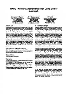
Fig. 2. Maritime trafficability values database.

not traversable and one indicates a region that is completely traversable. For the maritime applications considered here, these trafficability values are based on local traversability information and accounts for the following four “contextual” data: ² ² ² ²

Depth information, marked channel information, anti-shipping reports (ASR), and locations of high-value units (HVU).

The individual trafficability values corresponding to each contextual information are combined into a single value, which is used to indicate the repeller or attractor characteristic of a specific region. Details of this procedure are given next. First, a particular area of interest is divided into a grid-field, similar to a 15 £ 20 grid-field, as shown in Fig. 2. In Fig. 2, the purple channels indicate marked shipping lanes. As shown in Fig. 2, the area of interest contains three high-value units centered around cells (2, 11), (6, 14), and (11 : : : 15, 8). The area also contains two anti-shipping areas centered about cells (4, 2) and (5, 17). Finally, low-depth areas are mainly indicated using different shades of brown. According to the vehicle type that is being tracked, a single trafficability value, ºi , is assigned to each cell. This variable is a decimal 42

value between 0 and 1 and corresponds to the fraction of maximum velocity that the vehicle can attain in that grid location. For example, the grid cell (10, 17) has a trafficability of zero due to the depth information, and therefore, the vessels are supposed to avoid and navigate around this particular cell. Trafficability data is also used to deflect the direction of target motion given by the past velocity information. In order to implement this, at each propagation stage in the Con-Tracker, we consider a 3 £ 3 trafficability grid-field that depends on the current vehicle position. For example, if the vehicle is located in cell (13, 3), the 3 £ 3 trafficability grid-field consists of cells (12, 2), (12, 3), (12, 4), (13, 2), (13, 3), (13, 4), (14, 2), (14, 3), and (14, 4). A generic representation of the 3 £ 3 trafficability grid-field is shown in Fig. 3. The vehicle is assumed to be located in square 5 of the 3 £ 3 grid. The 3 £ 3 grid is continually re-centered about the vehicle as it moves throughout the region so that it is always located in the center (square 5) of the 3 £ 3 trafficability ˆ 2 R2 represents grid-field. In Fig. 3, the unit vector G tg the preferred direction of the vehicle strictly based on the trafficability information of the surrounding cells, ˆ ¡ 2 R2 is a unit vector in the direction of target motion G given by the past state information, and the unit vecˆ + 2 R2 represents the nudged velocity direction. A tor G


VOL. 6, NO. 1

JUNE 2011

where E[wk wTk ] = ¨ Qk ¨ T 2 ¢t3

ˆ ¡ is the direction of target Fig. 3. 3 £ 3 Trafficability grid-field: G ˆ + is the nudged ˆ is the preferred direction of target, G velocity, G tg velocity direction, and ºi indicate the trafficability of ith cell.

preferred direction based on the velocity constraint is calculated as P ˆ ˆ = ° j (ºj Gj )° G (1) tg P ° ˆ )° ° j (ºj G ° j

ˆ 2 R2 where j 2 f1, 2, 3, 4, 6, 7, 8, 9g. The unit vector G j points from the current vehicle location to the center of square j. Now the nudged velocity direction of motion is given as ˆ¡ ˆ ˆ + = G + ¹Gtg G (2) ˆ ¡ + ¹G ˆ k kG tg

where ¹ is a weighting coefficient that is calculated based on the absolute average difference in the trafficability values between the current location and the surrounding feasible locations P j jºj ¡ º5 j ¹= : (3) 8 Note that the proposed technique for determining the nudged velocity direction is chosen because it is least expensive in terms of computational requirements. 2.1. Filter Algorithm The theoretical developments of the Con-Tracker algorithm, which is based on the standard near-constant velocity tracker, are now shown. The state vector used in the filter is x 2 R4 , i.e., x = [¸ Á v¸

vÁ ]T

(4)

where ¸, Á, v¸ , and vÁ are the longitude and latitude locations of the target vehicle and the corresponding rates. In the case of the near-constant velocity models used in the ®-¯ tracker, zero-mean Gaussian white process noise is added to the model to account for the possible variations in velocity [7], [22]. Our approach modifies this concept by using the following discretetime model 2 3¯ ¯ ¸ + v¸ ¢t ¯ 6 7¯ Á + vÁ ¢t 6 7¯ 6 q 7¯ 7¯ xk+1 = 6 (5) 6 º5 v2 + v2 cos μ 7¯ + wk ¸ Á 6 7¯ 4 q 5¯ ¯ º5 v¸2 + vÁ2 sin μ ¯

6 3 6 6 6 0 6 =6 6 2 6 ¢t 6 q 6 2 1k 4 0

¢t2 q 2 1k

0

q 1k

3

¨ 2 R4£2

0

0

¢tq1k

¢t2 q 2 2k

0

and

Qk ´

3

7 7 7 ¢t q 2k 7 7 2 7 7 7 0 7 7 5 ¢tq2k 2

¢t q 3 2k

with

0

·

q 1k

0

0

q 2k

¸

:

The angle μ, the angle between the velocity vector and the local y-axis (north axis), defines the assumed ˆ + , i.e., direction of motion of the vehicle, G ˆ + = [cos μ G

sin μ]T :

(6)

ˆ + is determined using the trafficabilThe unit vector G ity data as explained in (2). The coefficient º5 is the q 2 2 trafficability of the current cell. The v¸ + vÁ term is simply the magnitude of the vehicle velocity and the trigonometric terms are used to project this value onto the appropriate axes. When no trafficability information is present, º5 defaults to one, and the trigonometric terms are given by v , cos μ = q ¸ v¸2 + vÁ2

vÁ sin μ = q v¸2 + vÁ2

(7)

which reduce (5) to the standard near-constant velocity ˆ ¡ in (2) model used in the ®-¯ tracker. Notice that the G is given as 3T 2 v Á ˆ ¡ = 4 q v¸ 5 : q (8) G 2 2 2 v¸ + vÁ v¸ + vÁ2 The measurement vector is assumed to be y = [¸ Á]T + [v¸

vÁ ]T

(9)

where v = [v¸ vÁ ]T is the zero-mean Gaussian whitenoise sequence, i.e., E[v] = 0 and E[vj vTk ] = R±jk . Let · ¸ 1 0 0 0 H= 0 1 0 0 then the measurement equation can be written as yk = Hxk + vk :

(10)

The near-constant velocity target model without the velocity nudging can be written in concise form as

k


xk+1 = ª xk + wk

(11) 43

where

2

1 0 ¢t

60 1 6 ª =6 40 0 0 0

0 1 0

0

TABLE I Summary of Con-Tracker Algorithm

3

¢t 7 7 7: 0 5 1

The estimation error covariance is defined as Pk = E[(xk ¡ xˆ k )(xk ¡ xˆ k )T ], and the following equations are used to propagate and update the error covariance matrix ¡ = ª Pk+ ª T + ¨ Qk ¨ T Pk+1

Initialize

xˆ (t0 ) = xˆ ¡ , P0¡ = E[(x0 ¡ xˆ ¡ )(x0 ¡ xˆ ¡ )T ] 0 0 0

Kalman Gain

Kk = Pk¡ H T [HPk¡ H T + R]¡1

Update

ˆ¡ ˆ¡ xˆ + k = xk + Kk [yk ¡ H xk ]

Velocity Nudging

ˆ¡= G

(12)

Pk+ = [I ¡ Kk Hk ]Pk¡

Kk =

¡1

+ R] :

k

¡ ¡ x+ k = xk + Kk [yk ¡ Hxk ]:

(16)

The Con-Tracker algorithm is summarized in Table I. Note that the Con-Tracker algorithm is very similar to that of a traditional Kalman filter-based tracking algorithm without the velocity nudging during the propagation stage. Since the process noise is added to the context-aware near-constant velocity model to account for variations in velocity, the process noise covariance Qk indicates the accuracy of target model in (5), i.e., how well a target complies with the given contextual information and the constant velocity assumption. If the target vehicle follows the model precisely, then Qk would be fairly small. If the vehicle maneuvers are erratic and inconsistent with the model, then the process noise covariance would be large. Since one does not know the precise value of the process noise covariance, an MMAE approach is implemented to estimate the process noise covariance based on the measurement residual. 3. MULTIPLE-MODEL ADAPTIVE ESTIMATION A brief overview of the MMAE approach is presented in this section. More details on the formulation of MMAE can be found in [4], [11], [42]. MMAE is a recursive estimator that uses a bank of filters that depend 44

(vˆ ¸+ )2 + (vˆ Á+ )2

P ˆ ) (º G °Pj j j ° ° (ºj Gˆ j )°

k

j

[cos μ

ˆ+ sin μ]T = G

¡ Pk+1 = ª Pk+ ª T + ¨ Qk ¨ T 2 ¸ˆ + + vˆ ¸+ ¢t

Propagation

3¯ ¯ ¯ ˆÁ+ + vˆ + ¢t ¯ 6 7 Á ¯ 6 7 ¡ xˆ k+1 = 6 p ¯ 7 4 º (vˆ ¸+ )2 + (vˆÁ+ )2 cos μ 5¯ ¯ p +2 ¯ + 2

(14)

The vector xˆ ¡ k is referred to as the a priori state estimate and the vector xˆ + k is referred to as the a posteriori state estimate. The estimates are propagated and updated using 3¯ 2 ¯ ¸ˆ + + vˆ ¸+ ¢t ¯ ¯ 7 6 7¯ 6 Áˆ + + vˆ Á+ ¢t ¯ 7 6 7¯ 6 q xˆ ¡ (15) + + k+1 = 6 º 7 2 2 (vˆ ¸ ) + (vˆ Á ) cos μ 7¯¯ 6 ¯ 5 4 q ¯ º (vˆ ¸+ )2 + (vˆ Á+ )2 sin μ ¯

p

#¯ ¯ ¯ p +2 ¯ (vˆ ¸ ) + (vˆ Á+ )2 ¯ vˆ Á+

vˆ ¸+

ˆ ¡ + ¹G ˆ ˆ+=G G tg

Pk¡

Pk¡ H T [HPk¡ H T

Pk+ = [I ¡ Kk Hk ]Pk¡

ˆ = G tg

(13)

ˆ¡ T = E[(xk ¡ xˆ ¡ where k )(xk ¡ xk ) ] is the a priori er+ ˆ+ T ror covariance and Pk = E[(xk ¡ xˆ + k )(xk ¡ xk ) ] is the a posteriori error covariance. The matrix Kk is the usual Kalman gain and can be calculated using

"

º

(vˆ ¸ ) + (vˆ Á ) sin μ

k

on some unknown parameters. In the problem under consideration, these unknown parameters are the process noise variances (diagonal elements of the process noise covariance) denoted by the vector qk = [q1k q2k ]T . For notational simplicity, the subscript k is omitted for q. Initially, a set of distributed elements is generated from some known probability density function (pdf) of q, denoted by p(q), to give fq(`) ; ` = 1, : : : , Mg. Here, M denotes the number of filters in the filter bank. The goal of the estimation process is to determine the conditional pdf of the `th element q(`) given the current-time measurement yk . Application of Bayes’ law yields p(Yk , q(`) ) p(q(`) j Yk ) = p(Yk ) p(Y j q(`) )p(q(`) ) = PM k (j) (j) j=1 p(Yk j q )p(q )

(17)

where Yk denotes the sequence fy0 , y1 , : : : , yk g. The probabilities p(q(`) j Yk ) can be written as p(q(`) j Yk ) = =

p(yk , Yk¡1 , q(`) ) p(yk , Yk¡1 ) p(yk j Yk¡1 , q(`) )p(Yk¡1 , q(`) ) : p(yk , Yk¡1 )

Since p(Yk¡1 , q(`) ) = p(q(`) j Yk¡1 )p(Yk¡1 ), p(q(`) j Yk ) can be written as p(q(`) j Yk ) =

p(yk j Yk¡1 , q(`) )p(q(`) j Yk¡1 )p(Yk¡1 ) : p(yk j Yk¡1 )p(Yk¡1 )


VOL. 6, NO. 1

JUNE 2011

Fig. 4. Uniform distribution and Hammersley quasi-random sequence comparison. (a) Uniform distribution. (b) Hammersley quasi-random sequence.

Now the probabilities p(q(`) j Yk ) can be computed through [4] p(y j xˆ ¡(`) )p(q(`) j Yk¡1 ) p(q(`) j Yk ) = PM k k ¡(j) ˆ )p(q(j) j Yk¡1 )] j=1 [p(yk j xk (18) xˆ ¡(`) ) k

(`)

in the since p(yk , j Yk¡1 , q ) is given by p(yk j Kalman recursion. The recursion formula can be cast into a set of defined weights $k(`) , so that (`) $k(`) = $k¡1 p(yk j xˆ ¡(`) ) k

(19)

$(`) $k(`) Ã PM k (j) j=1 $k

(20)

where $k(`) ´ p(q(`) j y˜ k ). The weights at time t0 are initialized to $0(`) = 1=M for ` = 1, 2, : : : , M. The convergence properties of the MMAE are shown in [4], which assumes ergodicity in the proof. The ergodicity assumptions can be relaxed to asymptotic stationarity and other assumptions are even possible for non-stationary situations [5]. The conditional mean estimate is the weighted sum of the parallel filter estimates xˆ ¡ k =

M X

$k(j) xˆ ¡(j) : k

(21)

j=1

Also, the error covariance of the state estimate can be computed using M X T ˆ ¡(j) ¡ xˆ ¡ Pk¡ = $k(j) [fPk¡ g(j) + (xˆ ¡(j) ¡ xˆ ¡ k )(xk k ) ]: k j=1

(22) The specific estimate for q at time tk , denoted by qˆ k , and error covariance, denoted by Pk , are given by M X qˆ k = $k(j) q(j) (23a) j=1

Pk =

M X j=1

$k(j) (q(j) ¡ qˆ k )(q(j) ¡ qˆ k )T :

(23b)

Equation (23b) can be used to define 3¾ bounds on the estimate qˆ k . At time t0 , all the filters have the same weight associated with them and there are many possibilities for the initial distribution of the process noise covariance parameters. A simple approach is to assume a uniform distribution. We instead choose a Hammersley quasirandom sequence [20] due to its well-distributed pattern. A comparison between the uniform distribution and the Hammersley quasi-random sequence for 500 elements is shown in Fig. 4. Clearly, the Hammersley quasirandom sequence provides a better “spread” of elements than the uniform distribution. In low dimensions, the multidimensional Hammersley sequence quickly “fills up” the space in a well-distributed pattern. However, for very high dimensions, the initial elements of the Hammersley sequence can be very poorly distributed. Only when the number of sequence elements is large enough relative to the spatial dimension, the sequence is properly behaved. This is not much of a concern for the process noise covariance adaption problem since the dimension of the elements will be much larger than the dimension of the unknown process noise parameters. 4.

L2/L3 HYPOTHESIS GENERATOR

As mentioned in Section 2, the estimated process noise covariance is indicative of how well the target vehicle follows the context-aware near-constant velocity model. If the target vehicle follows the model precisely, then the estimated process noise covariance would be fairly small, and if the vehicle maneuvers are erratic and inconsistent with the model, then the process noise covariance would be large. The incorporation of contextual data into the model allows variations in target vehicle velocity that are consistent with the given contextual information. For example, if the target vehicle in cell (7, 13) of Fig. 2 that is traveling toward cell (5, 15) makes a sharp right turn to avoid the high value unit in cell (6, 14), then the sudden change in the vehicle’s velocity is consistent with the contextual data provided, and therefore, would not result in an increase


45

in the estimated process noise covariance. However, if the target vehicle in cell (6, 3) that is traveling toward cell (3, 1) continues to travel in a straight line with a constant velocity, then there would be an increase in the estimated process noise covariance and the vehicle would be red-flagged despite its consistent behavior in accordance with the near-constant velocity model. This is because its passage into cell (5, 2) is in contrast to the anti-shipping activities reported in that area. Thus, a hypothesis on suspicious vehicle maneuvers can be synthesized based on the change in estimated process noise covariance. The near-constant velocity model combined with the trafficability information is given by 2 3¯ ¯ ¸ + v¸ ¢t ¯ 6 7¯ Á + vÁ ¢t 6 7¯ 6 q 7¯ 7¯ xk+1 = 6 (24) 6 º5 v2 + v2 cos μ 7¯ + wk : ¸ Á 6 7¯ 4 q 5¯ ¯ 2 2 º5 v¸ + vÁ sin μ ¯k

Any abrupt maneuver of the target vehicle that is inconsistent with the context-aware model can be treated as system process noise. This would, in turn, result in a sudden increase in the process noise covariance estimated by the MMAE. The two main objectives of the L2/L3 hypothesis generator is to red-flag a vehicle based on the anomalies in its behavior that are indicated by the change in process noise covariance and identify the reason behind the red-flagging. Since any anomaly in target behavior is indicated by a change in estimated process noise covariance, the proposed red-flagging algorithm is based on two sets of process noise covariance values. One set, fqˆ 1k , qˆ 2k g, is the MMAE estimate based on the Con-Tracker mea³ 1k , q ³2k g, surement residual values and the second set, fq is a second pair of MMAE estimates obtained using the standard Kalman filter-based tracker. The only difference between these two trackers is that the standard Kalman filter-based tracker does not make use of any contextual information. The second set of estimates, ³ 1k , q ³2k g, is used to normalize the first set of process fq noise covariance values. The normalized process noise covariances values are given as q¯ 1k =

qˆ 1k , ³ 1k q

q¯ 2k =

qˆ 2k : ³ 2k q

(25)

Normalization would eliminate any minor deviations in the process noise covariance values due to additive measurement noise. It also helps to clearly identify any abrupt maneuver of the target vehicle that is inconsistent with the given contextual information. After normalizing the elements of the process noise covariance matrix, their Euclidian norm is calculated as q kqk k = (q¯ 1k )2 + (q¯ 2k )2 : (26) 46

The rate of change of the normalized process noise covariance norm can be calculated as 1 (27) [kqk k ¡ kqk¡1 k]: ¢t The “change” in process noise covariance indicates the “occurrence” of target activity that is inconsistent with the prior knowledge. Therefore, a vehicle is red-flagged if the rate of change on the normalized process noise covariance norm is greater than a prescribed threshold, i.e., (28) ¢qk > ¢qmax ) Red-Flag: ¢qk =

Considering the rate of change of the normalized process noise covariance norm instead of the absolute magnitude helps to circumvent the slow transient response of the MMAE and thus, to avoid red-flagging a target long after the occurrence of an anomaly. A second red-flagging algorithm can be formulated based on a simple Â2 -test [7], [12], [35]. Suppose that a measurement residual is defined by ek = yk ¡ Hx¡ k, ¡ where yk is the measurement and Hxk is its corresponding estimate. For our case, the length of the measurement vector is m = 2, corresponding to longitude and latitude coordinates. The theoretically correct covariance associated with ek , denoted by Ek , can be derived from the Kalman filter equations, i.e., it is known from the Kalman tracking process. Define the following normalized error square (NES) "k = eTk Ek ek :

(29)

The NES can be shown to have a Â2 distribution with m degrees of freedom. A suitable check for the NES is to numerically show that the following condition is met with some level of confidence Ef"k g = m:

(30)

Typically, one writes the Â2 variable with its degrees of freedom as Â22 . A probability region can be constructed by cutting off the percent-difference upper tail. For example, a 99% probability region for a Â2 variance can be taken as the one-sided probability region (cutting off the 1% upper tail) [0,

Â22 (0:99)] = [0,

9:210]:

(31)

Other values can be found on page 84 of [7]. If the calculated Â2 value from (29) falls within this region, then an Â2 test indicates that the vehicle follows the Con-Tracker model with a high confidence of 99% and should not be red-flagged. The red-flagging reasoner deals with identifying the contextual information that is conflicting with the current target vehicle location. For example, the grid cell (2, 11) of Fig. 2 has a trafficability of zero due to the high-value unit location. Therefore, if a vehicle is located in cell (2, 11), then the conflicting contextual information is the high-value unit locations. Since the


VOL. 6, NO. 1

JUNE 2011

Con-Tracker is assumed to have access to all the contextual information, the simplest red-flagging reasoner can be synthesized by identifying which of the four contextual data contributes to the zero trafficability at the current location. The main assumption behind this approach is that there is only one piece of contextual information that is contributing to the zero trafficability at any specific time. A second red-flagging reasoner can be formulated as a hypotheses testing problem. Assuming that the hypotheses for the red-flagging reasoner problem can be stated as: ² H1 : Track is influenced by all contextual data except depth. ² H2 : Track is influenced by all contextual data except marked channels. ² H3 : Track is influenced by all contextual data except anti-shipping factor. ² H4 : Track is influenced by all contextual data except high-value unit factor. ² H5 : Track is influenced by all contextual data. Five different Con-Trackers can be designed according to the five different hypotheses given above. The hypothesis corresponds to the Con-Tracker that has the maximum likelihood value p(yk j x¡ k ) is selected as the candidate hypothesis. The a priori probability density function p(yk j x¡ k ) can easily be obtained from the appropriate Con-Tracker equations. 5. RESULTS In order to evaluate the performance of the a priori subsystem, a test case scenario is developed where we consider Hampton Roads Bay, Virginia, near the Norfolk Naval Station. The area of interest is first divided into a 15 £ 20 grid-field as shown in Fig. 2. Afterward, a trafficability value is assigned to each cell based on the target vessel type and the individual contextual data. Since we consider four different contextual data here, a combined trafficability value is also assigned to each cell by combining the four individual trafficability values. As shown in Fig. 2, the harbor area contains three high-value units centered around cells (2, 11), (6, 14), and (11 : : : 15, 8). The harbor area also contains two antishipping areas centered about cells (4, 2) and (5, 17). There are several marked shipping lanes in the harbor area that are indicated by shaded purple channels. For simulation purposes, we consider four different target vessels. 1) Two Ski Boats: Both ski boat tracks are indicated by red lines in Fig. 2. Details on the individual ski boats are given below: ² Ski Boat 1: Ski boat 1 starts in cell (15, 8) and travels toward cell (2, 1). Ski boat 1 crosses over two different marked channels at cells (14, 7) and (11, 5). Finally, the ski boat 1 crosses over a anti-shipping

Fig. 5. Ski boat 1 trajectories: Measured position (Meas), Con-Tracker estimate (ConT) & tracker estimate (Trac).

area located around cell (14, 2) and travels towards cell (2, 1). ² Ski Boat 2: Ski boat 2 starts in cell (15, 1) and travels toward cell (4, 20). Ski boat 2 crosses over a marked channel in cell (11, 7) and an anti-shipping area located around cell (5, 17) while traveling toward cell (4, 20). 2) Tugboat: Tugboat starts in cell (1, 20) and travels along the marked channel toward cell (13, 1). Its track is indicated by green lines in Fig. 2. 3) Sailboat: This boat is considered as a distressed vessel that is stranded in cell (7, 3) due to low water depth. For simulation purposes, the measurements are assumed to be obtained from an X-band coastal radar with a sampling frequency of 1/6 Hz. More details on state-of-the-art maritime surveillance technologies can be found in [48] and [47]. The measurement covariance is assumed to be of magnitude 1 £ 10¡7 to 2 £ 10¡7 . In the MMAE algorithm, 200 different filters are implemented using process noise covariance values in the range of 1 £ 10¡10 to 2 £ 10¡20 . The initial error covariance is selected to be 10¡6 £ I4 and the initial process noise covariance estimate is selected to be the ensemble mean of process noise covariance values. Details of the simulation results are given next. 5.1. Ski Boat 1 As shown in Fig. 2, ski boat 1 starts in cell (15, 7) and travels toward cell (2, 1). Fig. 5 shows the measured and estimated trajectories for ski boat 1. Fig. 5 contains the estimated trajectories from both context-aided ConTracker (denoted as ConT) and the traditional Kalman filter-based tracker (denoted as Trac). Fig. 6(a) shows the estimated process noise covariance variance values from the Con-Tracker/MMAE fqˆ 1k , qˆ 2k g and the Kalman ³ 1k , q ³2k g. The normalized process filter tracker/MMAE fq noise covariance norm, kqk k, is given in Fig. 6(b). Note


47

Fig. 6. Con-Tracker & tracker-estimated process noise covariance and normalized norm for ski boat 1. (a) Estimated q1 and q2 . (b) Normalized process noise covariance norm.

Fig. 7. Rate of change of normalized process noise covariance norm and trafficability values for ski boat 1. (a) Rate of change of kqk k. (b) Trafficability values.

the sudden increase in kqk k at times 50 sec, 150 sec, and 350 sec. The first increase in the process noise covariance values occur when the ski boat crosses over the marked channel located about cell (14, 7). The second increase in process noise covariance values occurs when the ski boat crosses over the second marked channel located about the cell (11, 5) at around 145 sec. The final increase in the process noise covariance values occurs when the ski boat enters the anti-shipping area located about cell (4, 2) at around 350 sec. Shown in Fig. 7 are the rate of change of normalized process noise covariance norm, ¢qk , and the trafficability values, º, for ski boat 1. The target vehicle (ski boat 1) is red-flagged based on the rate of change of normalized process noise covariance norm. The maximum allowable ¢qk is selected to be ¢qmax = 0:8. Note that at times 50 sec, 150 sec, and 350 sec, ¢qk is higher than its threshold value, and therefore, the target vehicle is red-flagged at these instances. Also note the low trafficability values at these instances as shown in Fig. 7(b). Fig. 8(a) shows μ, which is the angle between the velocity vector and the local y-axis, for the Con-Tracker 48

and the traditional Kalman filter-based tracker. The angle is measured positive clockwise and negative counterclockwise. Note that the angle obtained from the Kalman filter based tracker is much smoother compared to the one obtained from the Con-Tracker. The discrepancies in the Con-Tracker’s angle is due to the velocity nudging that occurs when the target vehicle encounters a zero-trafficability area. Also note that when the boat is traveling in a completely traversable region, μ obtained for the Con-Tracker and the traditional Kalman filter-based tracker are very similar. Fig. 8(b) shows the red-flag alerts for ski boat 1. Here, zero indicates a no red-flag alert and one indicates a red-flag occurrence. Note that the red-flag occurrence and the large deviations in μ are consistent with the results shown in Fig. 7. 5.2. Ski Boat 2 As depicted in Fig. 2, the second ski boat starts in cell (15, 1) and travels toward cell (4, 20). Fig. 9 shows the measured and estimated tracks for ski boat 2. Fig. 10(a) contains the estimated process noise covariance variance values from the Con-Tracker/MMAE


VOL. 6, NO. 1

JUNE 2011

Fig. 8. Con-Tracker & tracker-estimated direction and red-flag indicator for ski boat 1. (a) Boat direction. (b) Red-flag indicator.

Fig. 9. Ski boat 2 trajectories: Measured position (Meas), Con-Tracker estimate (ConT) & tracker estimate (Trac).

fqˆ 1k , qˆ 2k g and the Kalman filter-based tracker/MMAE ³ 1k , q ³2k g. Fig. 10(b) shows the normalized process fq noise covariance norm, kqk k, for ski boat 2. Note the sudden increase in kqk k at times 400 sec and 850 sec. The first increase in the process noise covariance values occurs when ski boat 2 crosses over the marked channel located about cell (11, 7). The second increase in the process noise covariance occurs when ski boat 2 enters the anti-shipping area located about cell (5, 17) around 850 sec. Shown in Fig. 11 are the rate of change of normalized process noise covariance norm, ¢qk , and the trafficability values, º, for ski boat 2. The maximum allowable ¢qk for ski boat 2 is also selected to be ¢qmax = 0:80. Note that at times 400 sec and 850 sec, ¢qk is higher than its threshold value, and therefore, the target vehicle would be red-flagged at these instances. Also note the low trafficability values at these instances as shown in Fig. 11(b).

Fig. 10. Con-Tracker & tracker-Estimated process noise covariance and normalized norm for ski boat 2. (a) Estimated q1 and q2 . (b) Normalized process noise covariance norm. ANOMALY DETECTION USING CONTEXT-AIDED TARGET TRACKING

49

Fig. 11. Rate of change of normalized process noise covariance norm and trafficability values for ski boat 2. (a) Rate of change of kqk k. (b) Trafficability values.

Fig. 12. Con-Tracker & tracker-estimated direction and red-flag indicator for ski boat 2. (a) Boat direction. (b) Red-flag indicator.

obtained for ski boat 1, the angle obtained from the Kalman filter-based tracker is much smoother compared to the one obtained from the Con-Tracker. The discrepancies in the Con-Tracker’s angle is due to the velocity nudging that occurs when the target vehicle encounters a zero-trafficability area. Fig. 12(b) shows the red-flag alerts for ski boat 2. Note that the red-flag occurrence and the large deviations in μ are consistent with the results shown in Fig. 11.

Fig. 13. Tugboat trajectories: Measured position (Meas), Con-Tracker estimate (ConT) & tracker estimate (Trac).

Fig. 12(a) shows the the angle between the velocity vector and the local y-axis, for the Con-Tracker and the Kalman filter-based tracker. Similar to the results 50

5.3 Tugboat The tugboat starts in cell (1, 20) and travels along the marked channel toward cell (13, 1). Fig. 13 shows the measured and estimated tracks for the tugboat. Fig. 14(a) contains the estimated process noise covariance variance values from the Con-Tracker/MMAE fqˆ 1k , qˆ 2k g and the Kalman filter-based tracker/MMAE ³ 1k , q ³2k g. Fig. 14(b) shows the normalized process fq noise covariance norm, kqk k, for the tugboat. Shown in Fig. 15 are the rate of change of normalized process noise covariance norm, ¢qk , and the trafficability values, º, for the tugboat.


VOL. 6, NO. 1

JUNE 2011

Fig. 14. Con-Tracker & tracker-estimated process noise covariance and normalized norm for tugboat. (a) Estimated q1 and q2 . (b) Normalized process noise covariance norm.

Fig. 15. Rate of change of normalized process noise covariance norm and trafficability values for tugboat. (a) Rate of change of kqk k. (b) Trafficability values.

Fig. 16. Con-Tracker & tracker-estimated direction and red-flag indicator for tugboat. (a) Boat direction. (b) Red-flag indicator.

Fig. 16(a) shows the the angle between the velocity vector and the local y-axis, for the Con-Tracker and the Kalman filter-based tracker. Fig. 16(b) shows the red-flag alerts for the tugboat. Note that there is no redflag occurrence for the tugboat since it remains in the marked shipping channel.

5.4 Sailboat A sailboat is considered as a distressed vessel that is stranded in cell (7, 3) due to low water depth. Fig. 17 shows the measured and estimated tracks for the sailboat. Fig. 18(a) contains the estimated process noise covariance variance values from the Con-Tracker/MMAE


51

noise covariance norm, ¢qk , and the trafficability values, º, for the sailboat. The maximum allowable ¢qk for the sailboat is also selected to be ¢qmax = 0:80. Fig. 20(a) shows the the angle between the velocity vector and the local y-axis, for the Con-Tracker and the Kalman filter-based tracker. Fig. 20(b) shows the red-flag alerts for the sailboat. Note that the red-flag occurrences of the sailboat are consistent with the low trafficability values given in Fig. 19(b). 6.

Fig. 17. Sailboat trajectories: Measured position (Meas), Con-Tracker estimate (ConT) & tracker estimate (Trac).

fqˆ 1k , qˆ 2k g and the Kalman filter-based tracker/MMAE ³ 1k , q ³2k g. Fig. 18(b) shows the normalized process fq noise covariance norm, kqk k, for the sailboat. Shown in Fig. 19 are the rate of change of normalized process

FINAL REMARKS

The objective of this work is to develop a contextaware target model and exploit available contextual information to provide a hypothesis on suspicious target maneuvers. The proposed concept involves utilizing the L1 tracking approach to perform L2/L3 situation and threat, refinement and assessment. A new context-aided tracker called the Con-Tracker is developed here. This tracker, which has its foundation in the standard Kalman filter based tracker, incorporates the available contextual information into the target vehicle model as trafficability values. Based on the trafficability values, the target

Fig. 18. Con-Tracker & tracker-estimated process noise covariance and normalized norm for sailboat. (a) Estimated q1 and q2 . (b) Normalized process noise covariance norm.

Fig. 19. Rate of change of normalized process noise covariance norm and trafficability values for sailboat. (a) Rate of change of kqk k. (b) Trafficability values. 52


VOL. 6, NO. 1

JUNE 2011

Fig. 20. Con-Tracker & tracker-estimated direction and red-flag indicator for sailboat. (a) Boat direction. (b) Red-flag indicator.

vehicle is either attracted or repelled from a particular area. Though the traditional Kalman filter-based tracker uses a near-constant velocity model, the Con-Tracker allows reasonable variations in velocity that are consistent with the contextual information. Any abrupt variations in velocity that is inconsistent with the contextaware target model would account for suspicious target maneuvers. Also, target maneuvers that are inconsistent with the given contextual information are also considered to be suspicious. Similar to the traditional Kalman filter-based tracker, the accuracy of the Con-Tracker estimates depends on the estimator parameters, such as the measurement noise covariance and the process noise covariance. While the measurement noise covariance can be readily obtained from sensor calibration, the process noise covariance value is usually treated as a tuning parameter. The proposed scheme utilizes a MMAE to estimate the process noise covariance value. Since the process noise is added to the near-constant velocity model to account for reasonable variations in velocity, target maneuvers involving large variations in velocity that are inconsistent with the contextual information would result in an increase in the estimated process noise covariance value. Based on the rate of change of the estimated process noise covariance values, an L2/L3 hypothesis generator red-flags the target vehicle. Simulation results indicate that the context-aided tracking enhances the reliability of erratic maneuver detection. There are several parts of the proposed scheme that can be further modified and improved. The current L2/L3 hypothesis generator uses the process noise covariance estimated using the MMAE approach. One of the main drawbacks of the MMAE approach is that it requires a long convergence period. Once the process noise covariance value increases due to an erratic vehicle maneuver, the MMAE approach requires the vehicle to travel through a perfect trafficability area for a long period of time before the process noise covariance value settles back at its initial low value. The convergence properties of the MMAE can be improved by incorporating correlations between various measurement times,

i.e., replacing the MMAE with the generalized MMAE (see [14]). The red-flagging design considered here depends on a threshold value for the rate of change of the normalized process noise covariance norm. A probabilistic red-flagging scheme, which integrates the current posterior error covariance and estimated process noise covariance, may be considered for future work. Finally, the accuracy and performance of the proposed scheme can be improved by considering more refined trafficability grid-field and more frequent and accurate measurements. ACKNOWLEDGEMENT This work was supported by Silver Bullet Solutions through an Office of Naval Research grant. The authors wish to thank David McDaniel and Todd Kingsbury from Silver Bullet Solutions for their support and generation of the data that was used in this paper. REFERENCES [1]

[2]

[3]

[4]

[5]

[6]


A. Alouani and W. Blair Use of a kinematic constraint in tracking constant speed, maneuvering targets. In Proceedings of the 30th IEEE Conference on Decision and Control, vol. 2, 1991, 2055—2058. A. Alouani and W. Blair Use of a kinematic constraint in tracking constant speed, maneuvering targets. IEEE Transactions on Automatic Control, 38, 7 (July 1993), 1107—1111. A. Alouani, W. Blair, and G. Watson Bias and observability analysis of target tracking filters using a kinematic constraint. In Proceedings of the Twenty-Third Southeastern Symposium on System Theory, 1991, 229—232. B. Anderson and J. B. Moore Optimal Filtering. Mineola, NY: Dover Publications, 1979. B. Anderson, J. B. Moore, and R. M. Hawkes Model approximations via prediction error identification. Automatica, 14, 6 (Nov. 1978), 615—622. Y. Bar-Shalom, K. Chang, and H. Blom Tracking a maneuvering target using input estimation versus the interacting multiple model algorithm. IEEE Transactions on Aerospace and Electronic Systems, 25, 2 (Mar. 1989), 296—300. 53

[7]

[8]

[9]

[10]

[11]

[12]

[13]

[14]

[15]

[16]

[17]

[18]

[19]

[20]

[21]

[22]

54

Y. Bar-Shalom, X. R. Li, and T. Kirubarajan Estimation with Applications to Tracking and Navigation. New York, NY: John Wiley & Sons, Inc., 2001. J. Barker, R. Green, P. Thomas, G. Brown, and D. Salmond Information fusion based decision support via hidden Markov models and time series anomaly detection. In 12th International Conference on Information Fusion, 2009, 764—771. H. A. P. Blom An efficient filter for abruptly changing systems. In The 23rd IEEE Conference on Decision and Control, Dec. 1984, 656—658. H. Blom and Y. Bar-Shalom The interacting multiple model algorithm for systems with Markovian switching coefficients. IEEE Transactions on Automatic Control, 33, 8 (Aug. 1988), 780—783. R. G. Brown and P. Hwang Introduction to Random Signals and Applied Kalman Filtering, 3rd ed. New York, NY: John Wiley & Sons, 1997, 353—361. B. Brumback and M. Srinath A chi-square test for fault-detection in kalman filters. IEEE Transactions on Automatic Control, 32, 6 (June 1987), 552—554. V. Chandola, A. Banerjee, and V. Kumar Anomaly detection: A survey. ACM Computing Surveys (CSUR), 41, 3 (2009), 1—58. J. L. Crassidis and Y. Cheng Generalized multiple-model adaptive estimation using an autocorrelation approach. In Proceedings of the 9th International Conference on Information Fusion, Florence, Italy, July 2006, paper 223. J. L. Crassidis and J. L. Junkins Optimal Estimation of Dynamic Systems. Boca Raton, FL: CRC Press, 2004. E. Daeipour and Y. Bar-Shalom An interacting multiple model approach for target tracking with glint noise. IEEE Transactions on Aerospace and Electronic Systems, 31, 2 (Apr. 1995), 706—715. M. Efe and D. Atherton Maneuvering target tracking using adaptive turn rate models in the interacting multiple model algorithm. In Proceedings of the 35th IEEE Conference on Decision and Control, vol. 3, 1996, 3151—3156. R. Fitzgerald Simple tracking filters: Position and velocity measurements. IEEE Transactions on Aerospace and Electronic Systems, AES-18, 5 (Sept. 1982), 531—537. A. M. Fosbury, T. Singh, J. L. Crassidis, and C. Springen Ground target tracking using terrain information. 10th International Conference on Information Fusion, July 2007. J. M. Hammersley Monte Carlo methods for solving multivariable problems. Annals of the New York Academy of Sciences, 86 (1960), 844—874. G. Jackson, L. Lewis, and J. Buford Behavioral anomaly detection in dynamic self-organizing systems: A cognitive fusion approach. In International Conference on Integration of Knowledge Intensive Multi-Agent Systems, Apr. 2005, 254—259. P. R. Kalata ®-¯; target tracking systems: A survey. In American Control Conference, 1992, 832—836.

[23]

K. Kastella and C. Kreucher Multiple model nonlinear filtering for low signal ground target applications. IEEE Transactions on Aerospace and Electronic Systems, 41, 2 (Apr. 2005), 549—564.

[24]

O. Kessler and F. White Data fusion perspectives and its role in information processing. In M. E. Liggins, D. L. Hall, and J. Llinas (Eds.), Handbook of Multisensor Data Fusion: Theory and Practice, Boca Raton, FL: CRC Press, 2009, ch. 2.

[25]

T. Kirubarajan, Y. Bar-Shalom, and K. Pattipati Topography-based vs-imm estimator for large-scale ground target tracking. In IEE Colloquium on Target Tracking: Algorithms and Applications, 1999.

[26]

T. Kirubarajan, Y. Bar-Shalom, K. Pattipati, and I. Kadar Ground target tracking with variable structure imm estimator. IEEE Transactions on Aerospace and Electronic Systems, 36, 1 (Jan. 2000), 26—46.

[27]

T. Kirubarajan, Y. Bar-Shalom, K. Pattipati, I. Kadar, B. Abrams, and E. Eadan Tracking ground targets with road constraints using an imm estimator. In Proceedings of IEEE Aerospace Conference, 5, 21—28 (1998), 5—12.

[28]

D. Lerro and Y. Bar-Shalom Interacting multiple model tracking with target amplitude feature. IEEE Transactions on Aerospace and Electronic Systems, 29, 2 (Apr. 1993), 494—509.

[29]

X. Li and Y. Bar-Shalom Design of an interacting multiple model algorithm for air traffic control tracking. IEEE Transactions on Control Systems Technology, 1, 3 (Sept. 1993), 186—194.

[30]

E. Mazor, A. Averbuch, Y. Bar-Shalom, and J. Dayan Interacting multiple model methods in target tracking: A survey. IEEE Transactions on Aerospace and Electronic Systems, 34, 1 (Jan. 1998), 103—123.

[31]

R. Moose, H. Vanlandingham, and D. Mccabe Modeling and estimation for tracking maneuvering targets. IEEE Transactions on Aerospace and Electronic Systems, AES-15, 3 (May 1979), 448—456.

[32]

A. Munir and D. Atherton Maneuvering target tracking using an adaptive interacting multiple model algorithm. In American Control Conference, 2 (1994), 1324—1328.

[33]

A. Munir and D. Atherton Adaptive interacting multiple model algorithm for tracking a manoeuvring target. IEE Proceedings–Radar, Sonar and Navigation, 142, 1 (Feb. 1995), 11—17.

[34]

P. O. Nougues and D. E. Brown We know where you are going: Tracking objects in terrain. IMA Journal of Mathematics Applied in Business & Industry, 8 (1997), 39—58.

[35]

J. Ouyang, N. Patel, and I. Sethi Chi-square test based decision trees induction in distributed environment. In IEEE International Conference on Data Mining Workshops, 15—19 (2008), 477—485.


VOL. 6, NO. 1

JUNE 2011

[36]

[37]

[38]

[39]

[40]

[41]

D. B. Reid and R. G. Bryson A non-Gaussian filter for tracking targets moving over terrain. In Proceedings of the 12th Annual Asilomar Conference on Circuits, Systems, and Computers, Pacific Grove, CA, Nov. 1978, 112—116. B. Ristic, B. La Scala, M. Morelande, and N. Gordon Statistical analysis of motion patterns in ais data: Anomaly detection and motion prediction. In 2008 11th International Conference on Information Fusion, 2008. M. Roemer, G. Kacprzynski, and M. Schoeller Improved diagnostic and prognostic assessments using health management information fusion. In IEEE Systems Readiness Technology Conference AUTOTESTCON Proceedings, 2001, 365—377. B. Salem and T. Karim Context-based profiling for anomaly intrusion detection with diagnosis. In Third International Conference on Availability, Reliability and Security, 2008, 618—623. R. Singer Estimating optimal tracking filter performance for manned maneuvering targets. IEEE Transactions on Aerospace and Electronic Systems, AES-6, 4 (July 1970), 473—483. S. Singh, H. Tu, W. Donat, K. Pattipati, and P. Willett Anomaly detection via feature-aided tracking and hidden Markov models. IEEE Transactions on Systems, Man and Cybernetics, Part A: Systems and Humans, 39, 1 (Jan. 2009), 144—159.

[42]

[43]

[44]

[45]

[46]

[47]

[48]

R. F. Stengel Optimal Control and Estimation. New York, NY: Dover Publications, 1994, 402—407. D. Sworder and R. Hutchins Maneuver estimation using measurements of orientation. IEEE Transactions on Aerospace and Electronic Systems, 26, 4 (July 1990), 625—638. D. Tenne and B. Pitman Tracking a convoy of ground vehicles. Center for Multisource Information Fusion, The State University of New York at Buffalo, Amherst, NY, Tech. Rep., Jan. 2002. D. Tenne, B. Pitman, T. Singh, and J. Llinas Velocity field based tracking of ground vehicles. Center for Multisource Information Fusion, The State University of New York at Buffalo, Amherst, NY, Tech. Rep., Aug. 2003. M. Ulmke and W. Koch Road-map assisted ground moving target tracking. IEEE Transactions on Aerospace and Electronic Systems, 42, 4 (Oct. 2006), 1264—1274. M. Vespe, M. Sciotti, and G. Battistello Multi-sensor autonomous tracking for maritime surveillance. In International Conference on Radar, 2008, 525—530. M. Vespe, M. Sciotti, F. Burro, G. Battistello, and S. Sorge Maritime multi-sensor data association based on geographic and navigational knowledge. In IEEE Radar Conference, 2008.

Jemin George received his B.S. (’05), M.S. (’07), and Ph.D. (’10) in aerospace engineering from the State University of New York at Buffalo. In 2008, he was a summer research scholar with the U.S. Air Force Research Laboratory’s Space Vehicles Directorate at Kirtland Air Force Base in Albuquerque, New Mexico. He was a National Aeronautics and Space Administration Langley Aerospace Research Summer Scholar with the Langley Research Center in 2009. From 2009— 2010 he was a research fellow with the Stochastic Research Group, Department of Mathematics, Technische Universitat Darmstadt, Darmstadt, Germany. He is currently with the Networked Sensing & Fusion Branch of the U.S. Army Research Laboratory. His principal research interests include stochastic systems, control theory, nonlinear filtering, information fusion, and target tracking. He is a student member of IEEE and AIAA. ANOMALY DETECTION USING CONTEXT-AIDED TARGET TRACKING

55

John L. Crassidis is a Professor of Mechanical and Aerospace Engineering at the University at Buffalo (UB), State University of New York, and also associate director for UB’s Center for Multisource Information Fusion. He received his B.S., M.S., and Ph.D. in mechanical engineering from the State University of New York at Buffalo. Prior to joining UB in 2001, he held previous academic appointments at Catholic University of America from 1996 to 1998 and Texas A&M University from 1998 to 2001. From 1996 to 1998, he was a NASA postdoctoral research fellow at Goddard Space Flight Center, where he worked on a number of spacecraft projects and research ventures involving attitude determination and control systems. His current research interests include nonlinear estimation and control theory, spacecraft attitude determination and control, attitude dynamics and kinematics, and robust vibration suppression. He is first author of the textbook Optimal Estimation of Dynamic Systems and has authored or coauthored more than 150 journal and refereed conference papers.

Tarunraj Singh received his B.E. degree from Bangalore University, Bangalore, India, his M.E. degree from the Indian Institute of Science, Bangalore, and Ph.D. degree from the University of Waterloo, Waterloo, ON, Canada, all in mechanical engineering. He was a postdoctoral fellow with the Aerospace Engineering Department, Texas A&M University, College Station. Since 1993, he has been with the University at Buffalo, Buffalo, NY, where he is currently a professor in the Department of Mechanical and Aerospace Engineering. He was a von Humboldt Fellow and spent his sabbatical at the Technische Universitat Darmstadt, Darmstadt, Germany, and at the IBM Almaden Research Center in 2000—2001. He was a National Aeronautics and Space Administration Summer Faculty Fellow with the Goddard Space Flight Center in 2003. His research has been supported by the National Science Foundation, Air Force Office of Scientific Research, National Security Agency, Office of Naval Research, and various industries, including MOOG Inc. Praxair and Delphi Thermal Systems. He has published more than 175 refereed journal and conference papers and has presented over 40 invited seminars at various universities and research laboratories. His research interests are in robust vibration control, estimation, and intelligent transportation.

Adam M. Fosbury received his B.S. in aerospace engineering and M.S. and Ph.D. in mechanical engineering from the State University of New York at Buffalo. From 2006 to 2007, he was a National Research Council Postdoctoral Research Fellow with the Air Force Research Laboratory Space Vehicles Directorate. In 2007, he became a full-time employee of the Air Force Research Laboratory. He left AFRL for the Johns Hopkins Applied Physics Laboratory in 2010 and is now performing guidance, navigation and control work for several spacecraft. He is currently a member of the AIAA Technical Committee on Guidance, Navigation and Control. 56


VOL. 6, NO. 1

JUNE 2011