Anonymizing Bipartite Graph Data using Safe ... - VLDB Endowment

Anonymizing Bipartite Graph Data using Safe Groupings Graham Cormode, Divesh Srivastava

Ting Yu, Qing Zhang∗

AT&T Labs–Research, Florham Park, NJ

North Carolina State University, Raleigh, NC

{graham,divesh}@research.att.com

{tyu,qzhang4}@ncsu.edu

ABSTRACT

them; much analysis can then be performed on structural properties of this graph. In this work, we study data that can be modeled as bipartite graphs—there are two types of entity, and associations link together one entity of each type. In the pharmacy, customers buy products, and in SIGMOD, authors write papers, building (customer, product) and (author, paper) associations. Each entity can be involved in few or many associations, but in most common situations, only a tiny fraction of all possible associations are present. In other words, the induced graph is quite sparse, and we must ensure that these associations are not easily revealed. Although the data is private, it is still desirable to allow aggregate analysis based on the structure of the graph. Pharmaceutical companies wish to understand which pattern of products are bought by people in particular age ranges; public health organizations want to watch for disease outbreaks affecting particular demographics based on certain types of medicine being purchased; SIGMOD may encourage analysis of hot topics in databases, or better understanding of coauthorship patterns. Publishing the raw data would allow these questions to be answered directly, but would fail to meet the privacy concerns outlined above. The model where the data owner accepts queries and either adds noise to results or refuses to answer some questions requires the data owner to be an active participant and may limit what analysis is possible. Instead, we adopt the approach of publishing some anonymized version of the data, and ensuring that the scope for inferring any given association from this data is limited while the key properties, in particular the structure of the underlying graph, is preserved. This approach allows a wide variety of ad hoc analyses and novel valid uses of the data, while ensuring our privacy goals are met. The problem of publishing anonymized data has attracted significant interest in recent years [7, 8, 9, 12, 13, 15, 16]. However, the focus has mostly been on tabular data, rather than the associations we study here. As a consequence, applying existing anonymization techniques tends to erase almost all structure, so that little use can be made of the resulting data. Moreover, a tabular approach ignores the inherent graph properties which hold a lot of the value of the data: e.g. structure such as number of customers buying the same product, pattern of other common products between customers using the same product, and so on. These are all important features of interest for aggregate analysis, but are radically altered by simply treating the data as a table and masking or perturbing the data. In Section 3, we work through several detailed examples to show that existing approaches for tabular data are insufficient for handling associations. Some recent work has begun to address anonymizing graph data, motivated by social network structure. Our work differs by making different assumptions about the strength of the attacker and the utility of the graph data: Prior work [1, 5] tends to assume a

Private data often comes in the form of associations between entities, such as customers and products bought from a pharmacy, which are naturally represented in the form of a large, sparse bipartite graph. As with tabular data, it is desirable to be able to publish anonymized versions of such data, to allow others to perform ad hoc analysis of aggregate graph properties. However, existing tabular anonymization techniques do not give useful or meaningful results when applied to graphs: small changes or masking of the edge structure can radically change aggregate graph properties. We introduce a new family of anonymizations, for bipartite graph data, called (k, `)-groupings. These groupings preserve the underlying graph structure perfectly, and instead anonymize the mapping from entities to nodes of the graph. We identify a class of “safe” (k, `)-groupings that have provable guarantees to resist a variety of attacks, and show how to find such safe groupings. We perform experiments on real bipartite graph data to study the utility of the anonymized version, and the impact of publishing alternate groupings of the same graph data. Our experiments demonstrate that (k, `)-groupings offer strong tradeoffs between privacy and utility.

1.

INTRODUCTION

Private data often arises in the form of associations between entities. An example is the products bought by customers at a pharmacy. The set of products being sold and their properties is public knowledge, and it may be no secret which customers visit a particular pharmacy. However, the association between a particular individual and a particular medication is often considered sensitive, since it is indicative of a disease or health issue that they have. A large example of association data is the Netflix prize data set, released in 2006, which was anonymized based on an unspecified heuristic method [2]. Another example is that of authors and papers: for a conference such as SIGMOD, reviewers learn information about submitted papers (title, area, abstract), and could (in future) also see detailed information about authors who have submitted papers, in order to verify conflicts of interest. But, since SIGMOD is a double-blind conference, the association between authors and papers should not be revealed to reviewers. The most natural way to model such data is as a graph structure: nodes represent entities, and edges indicate an association between ∗ Yu and Zhang were partially sponsored by the NSF through grants IIS0430166 and CNS-0747247.

Permission to make digital or hard copies of portions of this work for personal or classroom use is granted without fee provided that copies Permission to copy without feefor all profit or part or of this material is granted provided are not made or distributed commercial advantage and that copies are this not made distributed direct commercial thatthe copies bear noticeor and the fullforcitation on the firstadvantage, page. the VLDB copyright notice and the title of the publication andthan its date appear, Copyright for components of this work owned by others VLDB and notice is must givenbethat copying is by permission of the Very Large Data Endowment honored. Base Endowment. To copy otherwise, to republish, on servers Abstracting with credit is permitted. Toorcopy otherwise,totopost republish, or to redistribute to lists, requires a fee and/or special permission from the to post on servers or to redistribute to lists requires prior specific publisher, ACM. permission and/or a fee. Request permission to republish from: VLDB ‘08, August 24-30, 2008, Auckland, New Zealand Publications Dept., ACM, Inc. Fax +1 (212) 869-0481 or Copyright 2008 VLDB Endowment, ACM 000-0-00000-000-0/00/00. [email protected]. PVLDB '08, August 23-28, 2008, Auckland, New Zealand Copyright 2008 VLDB Endowment, ACM 978-1-60558-305-1/08/08

833

Customer c1 c2 c3 c4 c5 c6

State NJ NC CA NJ NC CA

(a) Customer table

Product p1 p2 p3 p4 p5 p6

Availability Rx OTC OTC OTC Rx OTC

(b) Product table

Customer c1 c1 c2 c2 c3 c3

Product p2 p6 p3 p4 p2 p4

Customer c4 c5 c5 c6 c6

Product p5 p1 p5 p3 p6

(c) Customer-Product table

c1

p1

c2

p2

c3

p3

c4

p4

c5

p5

c6

p6

(d) Graph Representation

Figure 1: Example data set lot of knowledge or power on behalf of the attacker (in particular, knowledge of node degrees, or of particular subgraphs), and shows that under such assumptions some associations can be inferred. In contrast, we address a different but equally important range of the privacy-utility tradeoff. We give a new approach for anonymizing associations which can be represented as bipartite graphs and show it to be resilient against certain attack models. Our Contributions. Our methodology is based on the idea that rather than masking or altering the graph structure, we should preserve the graph structure exactly, and instead focus on masking the mapping from entities to nodes of the graph. This approach ensures that the complex and sensitive graph structure is not affected, and so we can be sure that any analysis based principally on the graph structure will be correct. Privacy is ensured by grouping the nodes and entities: we partition the nodes in the graph, and the corresponding entities, into groups so that, given a group of nodes, there is a (secret) mapping from these nodes to the corresponding group of entities. There is no information published that would allow an attacker to work out, within a group, which node corresponds to which entity. This gives a tradeoff between privacy and utility: intuitively, larger groups give more privacy, but less certainty when answering queries which select a subset of entities. We give a simple condition for a grouping to be safe, which precisely limits the ability of an attacker to make any inference from the published information alone. We provide an algorithm which is successful at finding safe groupings in practice, and go on to describe how to answer a variety of query types efficiently given the published anonymized data. We also give formal analysis of how little can be deduced by an attacker who has additional background knowledge in the form of known associations between particular pairs of entities, and show that there is high security for entities about whom no information is known by the attacker. We demonstrate the efficacy of our approach with a careful experimental analysis of the ease of building safe groupings, and the accuracy with which a variety of queries can be answered over such anonymized data. We also study the effect of variations of our approach, and demonstrate that techniques based on publishing two versions of the same data, while significantly increasing the utility and accuracy of query answering, can also expose more associations to unintended revelation.

2. 2.1

were co-written by a set of authors; which websites were visited by users; which courses were taken by students; and so on. Throughout, we shall work with an illustrative example of a set of customers C = V and a set of products P = W . An edge (c, p) indicates customer c ∈ C bought product p ∈ P . Observe that here, as in many of the examples above, the graph is relatively sparse: each customer typically buys only a small fraction of all products, and each product is bought by only a few customers (with a few exceptions, e.g. many customers buy aspirin). As a consequence, the number of edges e is small compared to the number of possible edges, which is n × m. More formally, we say that a graph is α-sparse if e ≤ αnm; we will subsequently provide a necessary bound on the α-sparseness for our method to succeed. In full generality, we can consider graphs with multiedges, with weights or additional attributes. However, for clarity, we describe only the unweighted, undirected, single edge case: this has sufficient richness to capture many challenging problems. In a relational database, a bipartite graph G = (V, W, E) is naturally and concisely represented by three tables, corresponding to V , W and E. In our example, we would have a table of customers V , including attributes such as gender and location (from a customer loyalty scheme, say); a table of products W , including attributes such as price, type, and whether it is available Over the Counter (OTC) or by prescription only (Rx); and a customer-product table E encoding who bought what. Thus entities in the tables V and W correspond to nodes in the graph defined by E, in a 1:1 fashion. Example 1. Figure 1 shows a sample instantiation of this schema with Figure 1(d) showing the graph representation of the customerproduct relation in Figure 1(c). Customers have an additional attribute, state, indicating whether they are based in New Jersey (NJ), North Carolina (NC) or California (CA). The availability of a product indicates whether it is Over the Counter or Prescription Only. Since the graph accurately represents the relational data, we use both graph and relational terminology.

2.2

PRELIMINARIES Graph Model

Throughout, we focus on problems of anonymizing bipartite graphs G = (V, W, E) (bigraph for short). That is, the bigraph G consists of m = |V | nodes of one type, n = |W | nodes of a second type, and a set of |E| edges E ⊆ V × W . Such graphs can encode a large variety of data, in particular, the set of existing links between two sets of objects. For example, we can encode which documents

834

Privacy Goals

Our objective is to publish an anonymized version of the graph G, which still allows a broad class of queries to be answered accurately, but which maintains privacy of the associations. To make this goal precise, we describe our privacy goals, and outline classes of queries which we aim to answer. Our privacy objective is based on the idea that in many cases it is the association between two nodes which is private and must be disguised. As noted, the set of customers of a pharmacy may not be considered particularly sensitive, and the set of products which it sells may be considered public knowledge. However, the set of products bought by a particular customer is considered private, and should not be revealed. We focus solely on preserving the privacy of associations, and assume that properties solely of entities (e.g. state of a customer) are public. Clearly, there are situations with

differing privacy requirements, commented on in Section 7. Since it is desirable to allow answering of ad hoc aggregate queries over the data (e.g. how many customers from a particular zip code buy cold remedies), we wish to release some anonymized version of this data which gives accurate answers to such queries but protects the individual associations. More strongly, we want the graph properties of the data to be preserved. This corresponds to simple features, such as the degree distribution of the nodes, but also more long-distance properties, such as the distribution of nodes reachable within two steps, three steps, etc. Here, as in all work on anonymization, there is an inherent tradeoff between privacy and utility, although this can be hard to quantify precisely. Various extreme approaches maximize one over another: publishing the original data unchanged clearly maximizes utility, but offers no privacy; removing all identifying information and publishing only an unlabeled (“fully censored”) graph gives high privacy, but limited utility for aggregate queries over nodes satisfying certain predicates. Prior work has considered strong dynamic attack models (where nodes and edges can be inserted into the graph), which can result in some small number of associations being revealed [1]. For many situations we consider, this represents a very powerful attacker, and weaker attack models may suffice. It assumes that an attacker knows what data will be covered by the release and can easily modify it in advance. But, in the pharmacy example, adding edges means particular individuals must buy certain products in certain stores at certain times, which requires a very coordinated attacker. Adding nodes could involve creating new products for sale in the stores, which may not be plausible. Similarly, passive attacks require the attacker to collect complete and accurate information for a set of individuals. Even then, such attacks [1] only reveal information about entities for which some information is already known. Entities not involved in the attack remain secure. Clearly, there are cases where such attacks are possible and the results of [1] give a strong caveat; it is the responsibility of the data owner to determine against which attacks they should be secure. In extreme cases, the unlabeled graph structure leaks information about individual edges: for example, if the underlying graph is complete then we know there is an edge between any pair from the censored graph structure alone. Or, if there are a few nodes with unique degrees and these degrees are known to the attacker, these nodes can be reidentified. But in typical cases such as the examples we consider, virtually nothing can be deduced from the graph structure alone. Again, the data owner must determine whether this level of disclosure is acceptable to them. Here we aim for privacy guarantees relative to the baseline of the unlabeled graph. In particular, we study what guarantees can be made in the following scenarios:

same assumption is implicitly present in much of the prior work on anonymizing tabular data, such as k-anonymity and permutation based methods). We are still concerned when some negative inferences eliminate enough possibilities to leave a positive inference: learning c4 bought at least one item but did not buy p1, p2, p3, p4, or p6 allows us to infer that c4 did buy p5. This form of positive inference is specifically captured and limited by our analysis.

2.3

Query Types and Utility

As in prior work, given the difficulty of giving a precise privacy/utility tradeoff, we consider approaches which first fix a given level of privacy and then try to optimize and measure the utility. In order to more precisely analyze utility, we describe a set of sample aggregate query types which we wish to support. We will measure the utility of our results by studying the accuracy with which these queries can be answered using the anonymized data. The queries can be based on predicates over solely graph properties of nodes (such as degree), which we denote Pn , and predicates over attributes of the entities, Pa . In our customer-product example, Pa could select out customers from NJ, or prescription products, while a typical Pn might be that a customer buys a single product. We separate these two types of predicates, since when we publish a censored graph, we can still evaluate Pn predicates exactly, while we have maximum uncertainty in applying Pa predicates. We list a set of types of queries of increasing complexity, based on standard SQL aggregates (sum, count, avg, min, max): • Type 0—Graph structure only: Compute an aggregate over all neighbors of nodes in V that satisfying some Pn . E.g.: Find the average number of products per customer; Compute the average number of customers buying only that product, per product. • Type 1—Attribute predicate on one side only: Compute an aggregate for nodes in V satisfying Pa ; Compute an aggregate on edges to nodes in V satisfying Pn from nodes in W satisfying Pa . E.g.: Find the average number of products for NJ customers; Find total number of CA customers buying only a single product. • Type 2—Attribute predicate on both sides: Compute an aggregate for nodes in V satisfying Pa to nodes in W satisfying Pa0 . E.g.: Count total number of OTC products bought by NJ customers; Total sales of Rx products to CA customers who buy nothing else. Naturally, one can define yet higher orders of queries that are more complex, either through more constraints or more steps through the graph. Join-style queries would compute an aggregate of nodes from V at distance 2 from other nodes in V satisfying Pa connected via nodes in W satisfying Pa0 , and so on. One can also bring in other graph properties (such as measuring the diameter of an induced subgraph). For this work, we constrain our interest principally to the classes of queries defined above, since these are sufficiently rich to be challenging to answer accurately, while being sufficiently concise to specify compactly and work with over realistic data sets. In particular, note that while queries of type 0 can easily be answered on the fully censored graph exactly, answering queries of other types requires some more information about attributes of the entities in order to give any reasonable accuracy.

Definition 1. In the static attack case, the attacker analyzes solely the information which is published by the scheme, and tries to deduce explicit associations from this information. Ideally, the number of associations which can be correctly inferred (beyond what is implicit in the censored graph) should be minimal if not zero. In the learned link attack case, the attacker may already know a few associations — for example, that customer c1 bought p2. The additional associations that can be inferred should be minimal if not zero when the number of link revelations is small.

Datasets and Experimental Environment. All experiments for this paper were implemented in JDBC and SQL Server 2000. The primary dataset used is derived from DBLP and corresponds to all conference data. It was retrieved from http://dblp.uni-trier. de/xml/ on 06/21/2007, and is available on request from the authors. The data set contains |V | = 402023 distinct authors, |W | = 543065 distinct papers, and |E| = 1401349 (author, paper) edges. It represents the kind of association we are interested in,

We are principally concerned with an attacker being able to make positive inferences, e.g. being able to deduce that c6 bought p6. We are less concerned about negative inferences, e.g. deducing that c1 did not buy p1. Since the graphs we analyze are sparse, and the maximum degree at most a constant fraction of the total number of nodes, we consider such discovery to be entirely acceptable (the

835

Customer c1 c1 c2 c2 c3 c3 c4 c5 c5 c6 c6

Product p2 p6 p3 p4 p2 p4 p5 p1 p5 p3 p6

State NJ NJ NC NC CA CA NJ NC NC CA CA

Availability OTC OTC OTC OTC OTC OTC Rx Rx Rx OTC OTC

(a) Original data table

Customer * * * * * * * * * * *

Product * * * * * * * * * * *

State * * * * CA CA * * * CA CA

Availability OTC OTC OTC OTC OTC OTC Rx Rx Rx OTC OTC

(b) 3-anonymous data table

c1 c2 c3 c4 c5 c6 c1 c2 c3 c4 c5 c6

p1 0 0 0 0 1 0 p1 * 0 * 0 * 0

p2 1 0 1 0 0 0 p2 * 0 * 0 * 0

p3 0 1 0 0 0 1 p3 0 * 0 * 0 *

p4 0 1 1 0 0 0 p4 * * * * * *

p5 0 0 0 1 1 0 p5 * * * * * *

p6 1 0 0 0 0 1 p6 * * * * * *

(c) Matrix (top), 3-anonymized (bottom)

Figure 2: Attempting to apply existing anonymization to graph data with typical features (sparse graph, power-law degree distribution, non-random structure of links). We also carried out experiments on association data from other sources such as the IMDB (actors, movies), but in the interest of brevity, we only present results from DBLP, since other data gave similar conclusions.

3.

guarantee to anticipate all reasonable queries which could be formulated: recall that the purpose of publishing anonymized data is to allow a broad variety of ad hoc queries to be posed.

3.2

APPLYING EXISTING TECHNIQUES

A natural first approach to addressing these privacy questions is to apply prior work on table anonymization, since tables can represent graph data. However, such prior anonymization techniques only try to preserve the accuracy of table-based queries, and do not consider any graph semantics. As a result, we show that fundamental graph properties are quickly lost under such transformations, and we will see that even many of our type 0 queries are answered with intolerably high error. It is difficult to exhaustively try all existing methods, so we show that for three popular representative anonymizations that the results are not usable over graph data.

3.1

Representing as a relation

Representing the customer-product example in Figure 1 using tables, gives a customer relation (Figure 1(a)), a product relation (Figure 1(b)), and a customer-product relation (Figure 1(c)). We can join these to make a single table (Figure 2(a)), and try to anonymize it. In our example, each row lists a customer, a product, the customer’s state, and the product availability. How can we meet our goal of not revealing any (customer, product) association by applying a k-anonymization algorithm? Removing all customer IDs destroys all association structure from customers to products. Setting customer as a quasi-identifier and product as sensitive attribute fails because k-anonymization allows k products bought by the same customer to be grouped together (they share a quasi-identifier). Setting (customer, product) as the sensitive attribute fails, because kanonymization does not alter or mask sensitive attributes. Instead, we could add a dummy sensitive attribute of “true” to each row to indicate that the association is sensitive. The k-anonymized version of this table must use generalization and suppression to ensure each row is indistinguishable from k − 1 others [11, 12]. Options for concealing customer and product identifiers are limited: since they are arbitrary identifiers, there is no natural hierarchy for generalization so they can only be withheld. A 3-anonymized version of our example data set shown in Figure 2(b) provides very low utility. This attempt at anonymization loses the notion of individual customers and products, and so is unable to give useful answers to the query types outlined above. Augmenting the anonymized data with some additional information risks breaching privacy and does not

836

Representing as a matrix

A fundamental problem with the above approach is that k-anonymity is formally defined so that there should be at least k individuals whose representation is identical; in this representation, each individual is present in multiple places, so for example in Figure 2(b), two rows in the anonymized table refer to the same customer, giving them weaker privacy. This leads us to represent the graph data instead as a binary matrix: rows correspond to nodes in V , columns to nodes in W , and an entry (i, j) is set to 1 if there is an edge between vi ∈ V and wj ∈ W , and 0 otherwise. We can now take such a matrix, and try to apply existing anonymization techniques on it. Similar to above, the only meaningful anonymization of a 0 or 1 value is to generalize to “*”. Applying k-anonymization is similar to having customer as a quasi-identifier and product as a sensitive attribute [11, 12]: now products with more than k buyers may be revealed, while unpopular products may be fully masked. This also virtually wipes out the utility of the data. For example, Figure 2(c) shows the matrix representation of the sample data from Figure 1, and the result of 3-anonymizing it: all that is left is a few negative associations. The fundamental problem here is that these approaches have two equally unpalatable options: either an association is fully revealed, or else it is withheld.

3.3

Anonymization Through Permutation

A third approach to anonymizing tabular data is based on the idea of “permutation”: breaking the links between quasi-identifiable attributes and sensitive attributes [15, 16]. This seems more suited to the graph setting: we have an association between nodes in a graph that we wish to anonymize. This leads to the following algorithm: form edges into groups, and within each group, publish the pair of node (multi)sets that form edges. Grouping the edges from Figure 1 into sets of size 3 and 4 based on customer pairs gives: ({c1, c1, c2, c2}, {p2, p3, p4, p6}), ({c3, c3, c4}, {p2, p4, p5}), ({c5, c5, c6, c6}, {p1, p3, p5, p6}) Equivalently, for a group containing edges e1 = (v1 , w1 ), e2 . . . e` we generate ` permuted edges by picking a random permutation π and publishing e01 = (v1 , wπ(1) ) . . . e0i = (vi , wπ(i) ) . . . e0` . Conceptually, imagine taking every edge in the group and “breaking it in the middle”, then forming new edges by joining half-edges from V to half-edges from W . This method initially seems more promis-

y5 (p1)

x6 (c5)

y6 (p6)

(a) Grouped and Relabeled Graph

Group

y4 (p4)

x5 (c6)

Y-node

x4 (c3)

Group

y3 (p3)

X-node

x3 (c2)

Group

y2 (p2)

y2 y6 y1 y3 y4 y2 y4 y3 y6 y1 y5

Product

x2 (c4)

x1 x1 x2 x3 x3 x4 x4 x5 x5 x6 x6

Group

y1 (p5)

Customer

x1 (c1)

c1 CG1 p1 PG2 x1 CG1 y1 PG1 c2 CG1 p2 PG1 x2 CG1 y2 PG1 c3 CG2 p3 PG1 x3 CG1 y3 PG1 c4 CG1 p4 PG2 x4 CG2 y4 PG2 c5 CG2 p5 PG1 x5 CG2 y5 PG2 c6 CG2 p6 PG2 x6 CG2 y6 PG2 E0 HV HW RV RW (b) Published tables representing (3, 3) grouped graph

c1 c2 c4 c3 c5 c6

{ {

} }

p2 p3 p5 p1 p4 p6

(c) Graph of Published Data

Figure 3: (3,3)-anonymization of example relation ing than the above, since it guarantees to preserve node degrees (i.e. the number of products linked to a customer is the same before and after the permutation, and vice-versa), and the true mapping from customers to products seems well-masked. However, when we try to evaluate simple graph queries (type 0) over this data, we find that the results are highly inaccurate. To show this, we created a global permutation of the DBLP data where all edges are placed into a single group and permuted. We also created a small group permutation based on sorting papers primarily by conference and year and then by author count. Groups were defined by all edges relating to each consecutive pair of papers under this ordering. Figure 7(a) shows the result of plotting the distribution of the frequency of co-authorship for each pair of co-authors. The results clearly demonstrate that this permutation approach does not accurately maintain the coauthor relationship. In the source data 1.6M pairs of coauthors have written at least one paper together, and one pair has co-written 210 papers. In the global permutation, the maximum number of papers coauthored together is only three. The permutation of small groups is closer to the source distribution, but the error is still significant. This is unsurprising since coauthors often collaborate over long periods, writing multiple papers together. Permutation of papers breaks this correlation and links unrelated authors. All other grouping methods that we tried similarly failed to preserve these basic graph properties. Therefore we conclude that this approach gives very poor answers to simple type-0 queries, and so is not suitable for further consideration, since we next propose a method which guarantees perfect answers to type-0 queries.

4.

are met (proved in Section 4.3). We give a greedy algorithm to find a ‘safe grouping’ (Section 4.4) and then show how to answer queries given the published anonymized grouping (Section 4.5). Lastly, we consider a special case where some groups are revealed exactly (Section 4.6), and provide experimental results (Section 4.7).

4.1

Definition of Grouping

In this paper, we focus on masking the mapping via grouping the nodes of the graph. This technique preserves the underlying graph structure perfectly, but masks the exact mapping from entities to nodes, so for each node we know a set of possible entities that it corresponds to. The group size k is a parameter: larger k gives more privacy, but reduces the utility. We first provide formal definitions of groupings, illustrated by an example, and then show how these groupings enable the masking. Definition 2. Given a set V , a k-grouping is a function H mapping nodes to “group identifiers” (integers) so for any v ∈ V , the subset Vv = {vi ∈ V : H(vi ) = H(v)} has |Vv | ≥ k. Formally, ∀v ∈ V : ∃Vv ⊆ V : |Vv | ≥ k ∧ (∀vi ∈ Vv : H(vi ) = H(v)) That is, H partitions of V into subsets of size at least k. The kgrouping is strict if every group Vv has size exactly k or k + 1. In other words, a k-grouping partitions V into non-intersecting subsets of size at least k. The k-grouping ensures that each group is at least size k, to meet privacy goals; strictness ensures no group is much larger than k, for accuracy. We use the definition of grouping to publish a modified version of the graph: Definition 3. Let FV be a relabeling function to relabel elements of V injectively onto a new set FV (V ); and let FW be a relabeling function to relabel elements of W injectively onto a (disjoint) set FW (W ). Given a k-grouping on V , HV , and an `-grouping on W , HW , of a graph G = (V, W, E), define the (k, `)-grouped graph G0 as G0 = (V, W, HV , HW , E 0 , RV , RW ) where: (a) V and W are the original sets of entities V and W , and HV and HW are the grouping functions defined above. (b) E 0 is the relabeled edge set given by E 0 = {(FV (v), FW (w))|(v, w) ∈ E}. (c) RV , RW are remappings defined by RV (FV (v ∈ V )) = HV (v) and RW (FW (w ∈ W )) = HW (w). When both HV and HW are strict, this is a strict (k, `)-grouping.

PRIVACY THROUGH GROUPING

All the above attempts to use existing techniques render the data virtually unusable for the simple reason that they change or mask the graph structure in ways that fundamentally alter its properties. In contrast to the table case, where modifying a row has relatively minor impact on table properties, adding or deleting an edge can have significant impact on properties of a graph (for example, it can change a graph from being connected to disconnected). So we seek to avoid techniques which involve perturbing the graph structure. Instead, we focus on techniques which retain the entire graph structure but perturb the mapping from entities to nodes. That is, methods that publish a set of edges E 0 that are isomorphic to the original edges E, but where the mapping from E to E 0 is partially or fully masked. This technique is applicable in situations where it is considered safe to publish the unlabeled graph.

Example 2. For the example in Figure 1, set groups CG1, CG2 (customer group 1 and 2) and PG1, PG2 (product group 1 and 2) as −1 −1 (CG2) = {c3, c5, c6} (CG1) = {c1, c2, c4} HC HC −1 −1 HP (P G1) = {p2, p3, p5} HP (P G2) = {p1, p4, p6}

Outline. We define our grouping method in Section 4.1, and give a ‘safety’ condition in Section 4.2 which ensures that privacy goals

837

This is a strict (3, 3)-grouping since every customer group and every product group has (exactly) three members. The resulting grouped graph is shown in Figure 3(a), with the arbitrary relabeling of nodes on xi’s and yi’s. The published information can be derived from this: Figure 3(b) shows the five published tables (in addition to the original customer and product tables, Figure 1(a) and 1(b)). The result is compactly represented as a graph in Figure 3(c): it shows the edge structure, and which sets of nodes map to which sets of entities, but hides the exact mapping.

(m,n)

(1,n)

(k, l )

(m,1) Privacy

(1, l )

(m,1) U (1,n)

(k,1) U (1, l )

The grouping functions HV and HW contain most of the necessary information to specify the modified graph as a function of original graph G. This definition is well-suited to storage within a relational database. In the above example, we publish customer and product relations as before (corresponding to V and W ); customergroup and product-group tables which encode the mapping of each customer and product to groups (corresponding to HV and HW ); a masked-customer-product relation, in which each customer and product is mapped to a new node id (E 0 ); and lastly masked-customergroup and masked-product-group tables which map from the masked identifiers to groups (RV and RW ). Note that the base relations corresponding to V and W should not contain any information relating to the graph, such as the degree of the node. Otherwise, an attacker could potentially use this to relink between rows of V or W and nodes in E 0 . Two further examples of groupings illustrate extremes of the privacy-utility tradeoff: Example 3. Smallest groups. Setting HV (v) = v and HW (w) = w, (the identity functions) gives a (1, 1)-grouped graph G0 . Here, E 0 = E, and hence G0 encodes the original graph G exactly. Every query on G0 can be answered with the same accuracy as on G. So there is perfect utility, but no more privacy than we began with. Example 4. Largest groups. Setting HV to map all m = |V | members of V to the same group, say 0, and HW to map all n = |W | members of W to, say, group 1 gives the (m, n)-grouped graph G0 . G0 has no useful information mapping between entities in V, W and the nodeset of E 0 . That is, we publish entity tables and the fully censored graph. Recall that we are assuming it is acceptable to publish a censored graph, and so we say that this grouping guarantees the same level of privacy. This retains the graph structure, as required, but completely removes the mapping from entities (e.g. customers and products) to nodes in the graph. We cannot have any more privacy in our setting, when we insist on publishing at least this much information. This offers very limited utility in answering query types 1 and 2 listed in Section 2.3, since we cannot apply any selective attribute predicate with any certainty.

(k,1) Utility

(1,1)

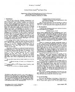
Figure 4: Lattice over groupings and privacy/utility tradeoff

4.2

Safe Groupings

There are many ways to form a k-grouping, but not all of these offer the same level of privacy, due to the local graph structure. We introduce the condition of ‘safety’ which ensures privacy holds even under revelation of certain information. Example 5. Consider a large graph G, which happens to contain the complete subgraph between nodes {v1 , v2 , v3 } and {w1 , w2 , w3 }. Suppose {v1 , v2 , v3 } forms the entirety of one group in HV , and {w1 , w2 , w3 } forms the entirety of a group in HW . From the published G0 , it is possible to infer immediately all the connections between these six nodes (a static attack). Such inference is not possible on the fully censored version of G0 , but the unfortunate choice of grouping allows information to leak. Some natural attempts to fix this, such as insisting that the density of edges between any pair of groups is low, are not guaranteed to still hold as edges are learned by an adversary. We define a stronger notion of ‘safe grouping’, which we subsequently prove is robust against static and learned link attacks. Definition 4. HV is a safe grouping of V in the context of a graph G = (V, W, E), if the following condition holds: ∀vi 6= vj ∈ V : HV (vi ) = HV (vj ) ⇒ 6 ∃w ∈ W : (vi , w) ∈ E ∧ (vj , w) ∈ E By extension, a (k, `)-grouping of a graph G is safe if HV and HW are both safe groupings. That is, a safe grouping ensures that any two nodes in the same group of V have no common neighbors in W (the definition for a safe grouping of W is symmetric, interchanging the roles of V and W ). This ensures a level of sparsity between groups, but goes further in restricting the pattern of allowed links. In the customerproducts example, it means that no two customers in the same group have bought the same product if the grouping is safe. Hence, the groupings in Figure 3 are safe. Given G and k > 1, there is no guarantee that there exists a safe k-grouping (all 1-groupings are trivially safe), but in practice they are easy to find (Section 4.4). A necessary condition for the existence of a safe (k, `)-grouping arises from the sparsity of the graph. A group of size k in V and a group of size ` together induce a subgraph of G which could have at most k` edges. However, if the grouping is safe then (within the induced subgraph) any node can have degree at most 1; otherwise, there are two nodes with a common neighbor. Figure 5(a) shows a typical structure between two groups of size k = 5 and ` = 6. So there can be at most min(k, `) edges between these two groups. This is true for every possible pair of groups. Since every

Privacy-Utility Tradeoffs. Between these two extremes lie many possibilities that trade off utility and privacy. Given a (k, `)-grouped graph, where both k and ` are fairly small, aggregate queries such as those described in Section 2.3 can be answered approximately. Bounds can be placed on the answers within which the true answer must fall (Section 4.5). When k and ` are small, these bounds are narrow; as k and ` grow large, the bounds will widen accordingly. Clearly, a (k, `)-grouping offers more utility (and less privacy) than a (k0 , `)-grouping if k < k0 ; the same holds true between (k, `)and (k, `0 ) groupings for ` < `0 . But we cannot easily compare (k, `)- and (k0 , `0 )-groupings unless k < k0 and ` < `0 . Thus, choices of k and ` define a lattice over possible groupings, bounded by (1, 1) and (m, n). We explore several points in this space in more detail; Figure 4 shows the lattice structure, including points of note that are defined and discussed in subsequent sections.

838

w with the anonymized nodes {x1 . . . xk} and {y1 . . . y`}. Since all k` possibilities are feasible, then there is an edge between v and w in exactly an e/k` fraction of feasible configurations, i.e. at most min(k, `)/k` = 1/ max(k, `), the bound on the density of the whole graph derived in Section 4.2. Since this analysis holds for every pair of groups, then the (static) attacker cannot infer any associations with certainty.

edge touches exactly two groups, the α-sparsity of the subgraph, defined by α = |E|/|V ||W |, can be at most min(k, `)/(k`) = 1/ max(k, `). Finding a k-grouping when all groups are forced to be size k can be hard even for small values of k: T HEOREM 1. Finding a safe, strict 3-grouping is NP-hard. P ROOF. Define G2 (V ) = (V, E 2 ) as the graph on V so that (vi , vj ) ∈ E 2 ⇐⇒ 6 ∃w ∈ W : (vi , w) ∈ E ∧ (vj , w) ∈ E. The requirement on HV to be safe is equivalent to requiring every pair of nodes in the same group form an edge in E 2 . That is, the group of nodes in the grouping forms a clique in (non-bipartite) G2 (V ). Therefore, a strict 3-grouping of V corresponds to a partition of G2 (V ) into triangles (forcing each group to be size 3). For any desired graph G1 = (V1 , E1 ), define a bigraph G = (V, W, E) such that G2 (V ) = G1 : create V = V1 and W ⊆ V × V , and for each (vi , vj ) ∈ E1 , insert (vi , (vi , vj )) and (vj , (vi , vj )) into E. Since partitioning a graph into triangles is NP-hard (problem [GT11] in [3]), and we can encode this problem as an instance of finding a safe, strict 3-grouping, we conclude that this problem is NP-hard also.

Under this measure, a (k, 1)-grouping offers the same static guarantee as a (k, k)-grouping. However, as we discuss in more detail in Section 4.6, there are other factors to consider. We remark on a connection to the concept of `-diversity [8]: here, the requirement is that between two groups the fraction of sensitive information (associations that are present) is bounded by 1/ max(k, `), which is similar to the `-diversity requirement. If there are small groups, the attacker’s confidence in a particular association can be higher. In particular, two groups of size 1 with an edge between them corresponds to a known association between entities. Although a safe (k, `)-grouping has no groups of size 1, in the active (learned link) attack model, when an attacker learns the existence of an edge (v, w), he may be able to refine the grouping in order to create groups of size 1. We will show that this refinement has bounded impact on the security of entities not directly impacted by the edge revelation, after presenting an example where an attacker may learn an association.

However, safe groupings can be found easily when the graph is sparse enough. For a bigraph G = (V, W, E) where every node has degree 1 (i.e. E gives a matching between V and W ), every possible grouping is safe, trivially. More generally, when the graph is sparse and does not have nodes which have (almost) all possible neighbors, safe k-groupings can be found for practical values of k (100 – 102 , say). Intuitively, the constraints posed by the edges of the graph are easy to satisfy when not too many edges are present. Most of the graph types discussed already are quite sparse and have few nodes of high degree: most shoppers purchase only a small number of the items on sale in a store, and most items are purchased by a fraction of all shoppers; most authors write only a small number of papers relative to the total number of papers written, and most papers have a small number of authors. Studying the data from DBLP, we observe that the most prolific author has written around 400 papers (out of 500K), and the most authors on a single paper is about 100 (out of 400K). In total, there are only 1.4M edges in the author-paper graph, out of a possible 400K × 500K = 200, 000M , demonstrating that typical association data is very sparse (α = 7 × 10−7 -sparse).

Example 6. Consider the four groups shown in Figure 5(c), and the three edges that connect them. Other nodes in the same groups have edges to other groups (dashed lines) which do not affect this example. In the static case, as proved above, the attacker cannot make any strong inferences. However, in the link learning case, if the attacker learns (t, v) is an edge, he can use the fact that there is only one edge between the group of t and the group of v to identify t and v with nodes in the anonymized graph. Likewise, learning (u, w) allows u and w to be identified with the nodes that represent them. As a consequence, the attacker can infer that (u, v) is an edge, no matter how many other nodes are in the groups. The example shows revealing an edge can maybe allow an attacker to learn more about the nodes that it connects, and so infer more about the connections between such nodes. But the amount revealed about entities for which the attacker does not have information is minimal. A relaxed grouping definition allowing a few groups of size one enables this intuition to be formalized.

4.3

Security of (k, `)-Groupings We analyze what can be deduced by an attacker presented with a safe (k, `)-grouping of graph data, where at least one of k and ` are greater than 1. We first argue that safe groupings are secure against the static attacks defined in Definition 1.

Definition 5. Define a (k, `)∗(p,q) -grouping as a grouping in which removing at most p nodes from V leaves a k-grouping of the remaining nodes of V , and removing at most q nodes from W leaves an `-grouping of the remaining nodes of W . Observe that a (k, `)-grouping is also a (k, `)∗(0,0) -grouping. Also, by applying Lemma 1, we note that a safe (k, `)∗(p,q) -grouping still gives a lot of privacy for nodes in the grouping: between a group of size k and one of size `, each possible edge is present in at most a 1/ max(k, `) fraction of possible configurations, as before. But also, between a group of size 1 and one of size `, there can be at most one edge in a safe grouping, and (also by Lemma 1) the edge is present in at most a 1/` fraction of possible configurations. Symmetrically, between a group of size k and one of size 1, the (at most one) edge is present in at most a 1/k fraction of possible configurations. Only between two groups of size one can we infer the existence (or absence) of an edge with certainty.

L EMMA 1. In a safe grouping, given nodes v ∈ V and w ∈ W in groups of size k and ` respectively, there are k` possible identifications of entities with nodes and the edge (v, w) is in at most a 1/ max(k, `) fraction of such possible identifications. P ROOF. Consider a group V G of V containing k nodes, and a group W G of W containing ` nodes. In the subgraph of G induced by V G and W G, there are e ≤ min(k, `) edges, following from the definition of safe grouping. There is no information available in what is published to break the symmetry between the nodes of V G, or between the nodes of W G. Recall, we insist that tables V and W contain no data related to the graph itself, such as degree or neighborhood, that could break this symmetry. For any entities v ∈ V G and w ∈ W G, it is feasible that (v, w) is an edge, and also feasible that (v, w) is not an edge. More strongly, consider the number of ways of identifying entities v and

T HEOREM 2. In the learned link case, given a safe (k, `)-grouped graph and r < min(k, `) true edges, the most an attacker can infer corresponds to a (k − r, ` − r)∗(r,r) -grouped graph.

839

Algorithm 4.1: G ROUP(V, W, E, k, j ← 0) repeat 8 for u8 ∈V > > > > > >i ← 1; > > > > > > > ∧(u, w) ∈ E) ∨ |V Gi | > k + j do > > > > > > < > : do i ← i + 1; V Gi ← V Gi ∪ u; > > j ← j + 1; V ← ∅; i ← 1; l ← 1; > > > > : (|V Gi(j−1) | > 0) >for i 8 > > > > > then V Glj ← V G ; l ← l + 1; > do > : : else V ← V ∪ V Gi(j−1) ;

c1 c4 t

v

c2

u

w

c3 c6

i(j−1)

c5

until |V | = 0

(a) Structure of safe groups

(b) Pseudocode to find safe k-grouping

} }

p2 p3 p5 p1 p4 p6

(c) (t, v) and (u, w) imply (u, v) (d) Safe (1, 3)-grouped graph

Figure 5: Safe Grouping Algorithm and Examples P ROOF. This is shown by induction over the revelation of r edges. The base case r = 0 yields the (k, `)∗(0,0) -grouped graph. In the inductive case, there is a (k − r, ` − r)∗(r,r) -grouped graph, and an additional edge (v, w) is learnt. As shown in the example above, in the worst case, this is enough to identify which node in the anonymized graph is v and which is w. This corresponds to refining of the groups: if v was in a group of size at least k − r, it is effectively split into a group of size 1 (containing v alone), and the remaining nodes now form a group of size at least k − r − 1. Likewise, the group containing w is split into one of size 1 containing w alone, and one of size at least ` − r − 1. The resulting grouping is therefore at least a (k − r − 1, ` − r − 1)∗(r+1,r+1) -grouping. Observe however, that the identification of v and w reveals nothing about any other nodes, even those connected to v and w. More precisely, the resulting grouping is still safe by Definition 4. The crucial observation is that any refinement of a safe grouping by partitioning groups into smaller pieces remains safe. By appealing to Lemma 1, the attacker cannot infer any associations beyond those that are revealed by the grouping directly (i.e. only those links between groups of size one). This is sufficient to bound the new knowledge by the (k − r, ` − r)∗(r,r) -grouping.

ordering of the nodes, or by picking a smaller value of k. Pseudocode of this heuristic is shown in Figure 5(b). In our experiments it was easy to find strict safe k-groupings for small values of k. There is the opportunity to optimize by choosing an initial ordering for the nodes, with the aim of giving better accuracy on queries. When a selective predicate is evaluated over a group, tighter query bounds are given when either (almost) all nodes in the group are selected, or none are selected. When a handful of nodes are selected from a group, there will be more uncertainty in answering the query. Putting similar nodes in a group together will therefore give higher accuracy. It is tempting to do this based on attributes of the entities. However, this can lead to attacks in the style of the minimality attack defined in [14]: knowing that groups were formed in a particular way allows an attacker to deduce the identity of nodes, and hence infer associations. Instead, if groups are chosen solely on graph properties, then we can publish the grouping algorithm, and anyone will find the same groups of nodes given the same unlabeled graph, so no information relating to the mapping of nodes to entities derives from the choice of which nodes to group together. This still gives many possibilities. For example, to improve accuracy on queries involving graph properties such as node degree (e.g. selecting customers buying a This is directly comparable to results on tabular data k-anonymization single product), sorting by node degree will greatly improve query answering. The sorted list of degrees of neighbors can break ties. where the aim is to ensure that individuals are secure up to the reveOther arrangements are possible; in our experimental evaluation lation of k − 1 pieces of information about other individuals. Here, we will compare the groupings found by an arbitrary ordering of individuals and their associations are secure up to the revelation of the nodes to one based on first sorting in the manner outlined. k − 1 pieces of information (edges) about others.

4.4

Finding a safe grouping

4.5

Query answering on (k, `)-grouped graph We show that aggregate queries of the type considered in Section 2.3 can be answered accurately and efficiently from a published (k, `)-grouped graph. First, since E 0 is isomorphic to E and queries of type 0 are solely on the underlying graph structure, they can be answered exactly. Queries of type 1 and 2 cannot guarantee perfect accuracy, since it is not possible to determine exactly which nodes their predicates select. However, they can be answered approximately, by providing bounds and expected values on the aggregate query. It is beyond the scope of this paper to cover all possible such queries, so we instead analyze various typical cases. A typical type 2 query is of the form “count the total number of OTC products bought in NJ”. Since the products within each group is known, the number of nodes selected by the product predicate in a group is easily found. The same is true for any customer group. The tightest bounds follow from evaluating the query over all possible assignments of entities to nodes, but this would be very costly, as the following theorem argues:

We describe a greedy algorithm to find a safe k-grouping of V . Precomputing the self-join of the edge table E on W allows quickly testing whether it is safe to put two nodes in the same group. For each node u in turn, the algorithm attempts to place u in the first group of the partial grouping with fewer than k nodes. If this would make the grouping unsafe, it tries the next group, and so on. If there is no group that meets these requirements, then a new group is started, containing u alone. After processing all nodes, there may be some (few) groups with fewer than k nodes in them. The algorithm collects these nodes together, and reruns the above loop allowing for groups of size k + 1 instead of k. If the graph is sufficiently sparse, then a safe grouping in which every group has either k or k + 1 nodes in is produced, and so the grouping is strict. Else, the algorithm continues but now allows groups up to size k + 2, and so on. Eventually, either a safe grouping is found, or the algorithm terminates once some large group size is reached. In this case, the method fails, but can be run again by choosing a different

840

T HEOREM 3. Finding the best upper and lower bounds for answering an aggregate query of type 2 is NP-Hard.

As above, since we have to do a constant amount of work for each edge in the original bigraph, the computational cost is O(|E|).

P ROOF. The hardness of the tight upper bound problem is shown by a reduction from the set covering problem [3]. Given subsets S1 , . . . , St , whose union is U = {a1 , . . . , au }, construct a bipartite graph (V, W, E). For each subset Si , create a node vi in V . All nodes in V are placed into a single group of size t. For each ai ∈ Sj , create a node wij in W , and an edge (vj , wij ). W is partitioned into groups corresponding to the same ai , i.e., group Gi = ∪j {wi,j }. The grouping of the graph is safe, by construction. To decide whether there exists k subsets that cover U , we set our problem as follows: the query selects k nodes in V , and exactly one node from each group of W . There is a set cover of size k if and only if the answer to the tight upper bound problem is |U |. The hardness of the tight lower bound problem is shown by a reduction from the maximum independent set problem [3]. Given an undirected graph G1 = (V1 , E1 ), construct a bipartite graph G0 = (V, W, E 0 ) similarly to the proof of Theorem 1: for each edge (vi , vj ) ∈ E1 , insert (vi , (vi , vj )) and (vj , (vj , vi )) into E 0 , and create a group of size 2 containing the two nodes (vj , vi ) and (vi , vj ). All nodes in V are put in a single group. Again, the grouping of G0 is safe by construction. To decide if there exists an independent set of size k in G, set the query to select k nodes in V , and only one node in each group of W . There is an independent set of size k if and only if the tight lower bound for this query is 0.

4.6

(k, 1)- and (1, `)-Groupings A significant class of groupings arise when all groups of one set of nodes are of size 1. These are (k, 1)- (or symmetrically, (1, `)-) groupings. Here, more is revealed about associations between entities of the same type (our focus up to now has been on associations between entities of differing types), since the true mapping from one set of nodes to entities is revealed. In the customer-products example, a (1, `)-grouping reveals exactly how many products a particular customer has bought, who has bought the same product, etc., while still protecting the exact associations. Example 9. Figure 5(d) shows a safe (1, 3)-grouping of our example data. The corresponding published tables are HW and RW as shown in Figure 3(b); HV and RV are not needed, since V maps directly onto the nodes of E 0 . Despite this information being revealed, the private associations between customers and products are still hidden: although Figure 5(d) shows that customers c1 and c3 bought the same product, it could be any one of {p2, p3, p5}. This again resembles `-diversity: any customer is known to have bought one product out of `. From Lemma 1 and Theorem 2, given a safe (k, 1)-grouping, any edge still is between one of k equally likely nodes of V , and given r edge revelations, an attacker is still faced with a (k − r, 1)∗(r,0) -grouped graph. While information is revealed about interactions between one set of nodes (customers, in the example above), in many cases, this information release may be permissible. If so, higher accuracy on queries is possible.

Instead, slightly weaker bounds are obtained by considering each pair of groups in turn to find bounds on the query answer: Example 7. Consider answering the query “Count the total number of OTC products bought in NJ”. Given a safe group CGi of ki customers, of whom ai are NJ customers; a safe group P Gj of `j products, of which bj are OTC products; and cij edges between the two groups: (i) There can be a contribution of at most Ui,j = min(ai , bj , cij ) to the query (Upper Bound). The totalP contribution over all customer groups CGi is at most Uj = min( Pi Ui,j , bj ), and the final bound over all product groups is U = j Uj . (ii) There is a contribution of at least Li,j = max(0, ai + bj + cij − ki − `j ) to the query (Lower Bound), and the bound over all customer groups is Lj P = maxi Li,j . We can sum this to get the overall lower bound, L = i Li . (iii) Treating all assignments of nodes to entities as equally likely, the expected selectivity between CGi and a b c P Gi is Eij = ik j`2ij (Expected Bound). Over all groups, the estii j Q mated expected bound is Ej = `j (1− i (1−Ei,j )), assuming independence and using inclusion-exclusion principle. The expected P bound for the query is then E = j Ej . These can be verified by simple case analysis over the structure in Figure 5(a).

Query answering on (1, `) and (k, 1)-grouped data. Queries are answered in much the same way as in the more general (k, `) case. However, many queries are answered more accurately, since the amount of uncertainty is reduced: in Examples 7 and 8, ai = ki = 1 or bj = `j = 1, simplifying the bounds. In particular, some queries of type 1 can be answered exactly: if the predicate is on the 1-grouping, the correct set of entities can be found exactly, which allows the exact answer to the aggregate query to be found. Type-2 queries can be answered with tighter bounds: Example 10. For the query of Example 7 over a (k, 1)-grouped graph, the set of OTC products is known precisely. For each OTC product, we add 1 to the upper bound if they have a buyer in a group which contains an NJ customer; and add 1 to the lower bound if they have a buyer in a group in which everyone is in NJ. For the expected bound, the expectation that a customer in a group of size ki with ai NJ customers is Ei,j = ai /ki , so Q the probability of any buyer of the product being from NJ is 1 − i (1 − Ei,j ). Similarly, for Example 8, we can consider all single products bought by NJ customers exactly, and find the corresponding bounds (upper, lower, and expected) on which are prescription only.

Such queries can be answered in time O(|E|), since each edge in the original graph connects a single pair of groups, and for groups with no edges between them (cij = 0), Ui,j = Li,j = Ei,j = 0. Example 8. The query “Find the maximum number of CA customers buying a single Rx product” can be answered by considering in turn each node that could possibly be a CA customer (is in a group which contains at least ai ≥ 1 CA customers), and finding exactly the products bought alone associated with that node. Upper and lower bounds increase by one if there are bj ≥ 1 Rx products or fewer than `j Rx products in the product’s group of size `j , respectively. These imply upper and lower bounds on the global maximum. Similarly, expected bounds follow by assuming a customer has probability of being in CA with probability ai /ki in a group of ki customers; and that a product in a group of `j product has probability bj /`j of being prescription only.

4.7

Experimental Analysis of Utility

In this section, we evaluate the utility of the anonymized data through experiments on the DBLP data. Specifically, we study the accuracy of three queries with different properties. For each query, we compute the lower bound estimation L, the upper bound estimation U , and the expected value µ. If the correct answer to the query is Q, we compute two error measurements: the error bounds U −L (the worst case error from using (U + L)/2 as an estimate for 2Q Q), and the expected error |µ−Q| . To clearly show the trends, we Q repeat each experiment over ten random choices of predicates and show the mean error bounds. The three queries are:

841

Query A Error Bounds

Query B Error Bounds 150

100

50

0

Query C Error Bounds 150

(20,20)-grouping (10,10)-grouping (5,5)-grouping

Error Bounds %

(20,20)-grouping (10,10)-grouping (5,5)-grouping

Error bounds %

Error bounds %

150

100

50

0 10

30

50 70 Pa Selectivity %

(a) Query A

90

(10,10)-grouping (1,10)-grouping (10,1)-grouping

100

50

0 10

30

50 70 Pa Selectivity %

(b) Query B

90

10

30

50 70 Pa Selectivity %

90

(c) Query C, Pa0 selectivity 0.8

Figure 6: Impact of query selectivity and group size on three queries • Query A: Find the average number of authors of any paper satisfying predicate Pa . This is a type-1 query with an attribute predicate only. We vary the selectivity of Pa from 10% to 90%.

For Query C (Figure 6(c)), there is little variation as Pa ’s selectivity varies (in this plot, selectivity of Pa0 is set to 0.8; similar experiments for other values of Pa0 are omitted for space reasons). Note that when we have a paper group of size 1, as in the (10, 1)grouping, we can directly select out exactly those papers that meet the predicate, and so have better accuracy compared to other groupings. There is little difference between the (10, 10)-grouping and the (1, 10)-grouping. This is because Pa0 selects most authors, so there is not much benefit from the (1, 10)-grouping’s ability to eliminate some candidates. When Pa0 selects fewer authors, there is a clearer advantage of (1, 10) over (10, 10) grouping. Expected Case Error Bounds. Although the above worst case bounds show that there can be a wide range between the upper and lower bounds on a query, we show next that the expected bound can give a quite accurate answer. Figures 7(b) and 7(c) show the expected error on queries B and C (the expected error on query A was too close to zero to plot). The general trend is again that higher values of selectivity give better accuracy. However, observe that the expected errors are much smaller than the worst case bounds, and do not vary much based on group size—in several cases a larger grouping achieves better expected error than a smaller one. On query C, as in the worst case, the expected error is much smaller on (10, 1) than (1, 10) or (10, 10), which are about the same for this (more selective) Pa0 ; similar results occur for other values of Pa0 . Impact of ordering on grouping. Query 2 involves a structural predicate (single author papers), so we compare ordering the grouping by degree and second-order degree to an arbitrary grouping in Figure 7(d). We see that there is a very dramatic benefit to having a grouping based on this ordering: two orders of magnitude improvement in the accuracy. This is because most groups now contain papers with the same number of authors, meaning the contribution to the aggregate can be found exactly for those groups, and the few that remain contribute to the uncertainty. We further investigate the impact of the correlation of the predicate with the grouping. For query B, we construct an artificial predicate Pa which selects the same number of total papers, but touches a variable number of papers in each paper group within a (5, 5) grouping. Figure 7(e) shows that as the number of papers touched in each group increases, both the expected and worst case bounds improve up to the point when all papers are selected in a group, the aggregate query is answered with perfect accuracy. This shows that if we can anticipate the kinds of structural predicates that end users will want, then we can improve the utility of the published data without compromising the privacy.

• Query B: Find the total number of single author papers satisfying Pa . This is also a type-1 query with both attribute predicates and structural predicates. The selectivity of Pa is varied as above, while the single author predicate is held constant. • Query C: Find the total number of papers satisfying Pa having authors who satisfy Pa0 . This is a type-2 query. We vary the selectivity of both Pa and Pa0 . These fit exactly the form of the queries we have studied in Example 7 and Example 8 (note that type-1 queries can be thought of as type-2 queries where one of the attribute predicates is always true). We do not consider any type-0 queries, since our earlier analysis shows that they can be answered exactly from the graph structure alone. We computed groupings over the papers and authors in the DBLP data described in Section 2 using the method detailed in Section 4.4. We built 20-groupings, 10-groupings, and 5-groupings over the data. The first iteration of the algorithm was able to find safe k-groupings covering almost every node: the 20-grouping of papers had 43 papers (out of 540K) not in groups of size 20, while there were just 3 authors not in groups of size 20. The next iteration easily found a safe, strict 20-grouping. The following parameters can impact query accuracy: • Group size: We compare approaches from (k, 1)-, (1, `)and (k, `)-groupings. We expect smaller group sizes to offer better accuracy for query answering. • Selectivity of predicates: More highly selective queries are more likely to touch just a few nodes within a single group, and so lead to wider worst case bounds. • Grouping formation: We will study the impact of building the groupings based on an arbitrary initial ordering of the nodes, and based on sorting based on degree and neighborhood degree, as discussed in Section 4.4. We expect sorted groupings to give better answers when queries have structural predicates based on degree. Worst Case Error Bounds. Figure 6 shows the worst case error bounds for query answering with (k, k)-groupings over the queries A, B, and C. As expected, smaller groupings achieve smaller uncertainty. There is also a clear trend for Queries A and B (Figure 6(a) and 6(b)) that as the selectivity of Pa increases, the accuracy improves. When only a single node in a group is touched by a query, as happens when selectivity is low, it could be any node, and so we have high uncertainty for the aggregate value in the group. But when many nodes are selected in a group, there is less relative uncertainty for an aggregate like sum or average.

5.

842

UNIONS OF GROUPINGS

Query B Expected Error 20

5

10

104 103 102

(5,5)-grouping (10,10)-grouping (20,20)-grouping

15 10 5

(1,10)-grouping (10,10)-grouping (10,1)-grouping

15 10 5

1

10

0 101 102 Number of Papers

0 10

103

30

50 70 Pa Selectivity %

(d) Impact of Grouping Order

90

10

Relative Error % 90

0.8

50

0.6 0.4 0.2

0 3

4

90

Distribution of Author Identifiability

100

2

50 70 Pa Selectivity %

1

Worst Case Expected

1

30

(c) Expected Error Query C, Pa0 selectivity 0.1

Impact of Predicate-Grouping Correlation 150

(20,20) random (5,5) random (20,20) sorted (5,5) sorted

10

50 70 Pa Selectivity %

(b) Expected Error on Query B

Impact of Grouping Order 105 104 103 2 10 101 100 10-1 -2 10 10-3

30

Fraction

100 0 10

(a) Type-0 queries on permuted tables

Expected Error %

Query C Expected Error 20 Expected Error %

Original Distribution Group Permutation Global Permutation

106

Expected Error %

Number of Coauthor Pairs

Distribution of Coauthorship Frequency 107

0 0 10

5

4-step 3-step 2-step 1-step 1

10

2

10

Number of Nodes Touched per Group

(e) Correlation between predicate and groups

10 k

3

10

4

5

10

6

10

(f) Attacking a (m, 1) ∪ (1, n)-grouping

Figure 7: Experiments on Grouping and Clustering In this section, we consider the impact of publishing multiple groupings of the same graph. This allows a broader class of queries to be answered with perfect accuracy, but is open to stronger classes of attack based on the graph structure. Recall that publishing the fully-censored (m, n)-grouped graph allows type-0 queries to be answered exactly, but gives us no handle to answer other query types with certainty. As observed in Section 4.6, publishing (1, `) or (k, 1) grouped graphs offers greater utility for a variety of queries while preserving the privacy of associations. So it seems that publishing both, as a (1, `) ∪ (k, 1) grouping of a graph, is desirable, since any query of type 1 could be answered exactly. But while either version of the graph in isolation is resilient against attack, publishing both allows an attacker to combine the information in the static attack model (Definition 1), as they now have information not previously available to them. If a customer has bought more products than any other, she can be identified statically from the (1, `) graph, i.e. with no background knowledge about degrees or other data. From its unique degree, the same node can be located in the (k, 1)-grouped graph, revealing all the products bought by that customer. This attack applies even over (m, 1) ∪ (1, n)-grouping, which give the most privacy in this class. More strongly, if certain types of mappings between the isomorphic (m, 1) ∪ (1, n)-grouped graphs can be found, the original data can be recovered. This problem is related to, but distinct from, the (well-studied) graph isomorphism problem. Some information will remain private: associations for customers who have only ever bought a single bespoke product unique to them cannot be recovered from (k, 1) ∪ (1, `)-grouped graphs, even though finding a valid isomorphism over these nodes is easy. But if the attacker can find node or edge pairs that must be uniquely mapped to each other in every isomorphism, their privacy is compromised. Clearly, the amount of privacy that remains is input dependent: data consisting solely of nodes with degree 1 is secure; but if each node has a unique degree then total re-identification is trivial. On realistic

data, the truth lies somewhere in between. Experimental Analysis of Privacy. We attack (m, 1) ∪ (1, n)grouped graphs, based on finding matching pairs of nodes between the two graphs. Each node in the fully censored graph is given a compact signature. Initially, the signature of every node is a default value, say 0, since there is no a priori way of telling them apart. Given a node, its next-step signature is formed by concatenating its current signature with the signatures of all its neighbors in the graph, and sorting this set lexicographically. Once next-step signatures are found for all nodes in the graph, they can be compactly relabeled (since there can be at most n different signatures for n nodes). By this construction: (a) If two nodes have different signatures then they cannot be matched in any isomorphism—since the signature canonically encodes features of the neighborhood of a node, different signatures entail non-isomorphic neighborhoods. (b) Since the process is entirely deterministic, each node will obtain the same signature every time the procedure is run on the graph. As a result, if a node receives a signature that is not shared by any other node, then this node must be uniquely matched in any isomorphism. Moreover, it can be matched to the unique node with the same signature in an isomorphic copy. Note that the implication is only one way: the guarantee is that if signatures are unique then nodes can be uniquely matched, and not vice-versa. We apply this signature scheme on the (m, 1) ∪ (1, n)-grouped graphs, and measure how many nodes are uniquely identified, and how many fall into equivalence classes of size 2, 3, 4 etc. The cumulative distribution over such classes of authors in the DBLP dataset are shown in Figure 7(f). Multiple steps of signature computation were performed, but on this data (and on similar datasets such as IMDB), no improvement was seen after the fourth iteration, and there is only limited difference from the third to fourth step. A 4-step signature is sufficient to identify half of authors uniquely, and only 20% are in equivalence classes of 10 or larger. Such privacy levels are weak for many typical applications, so we conclude

843

that (1, `) ∪ (k, 1)-groupings should be avoided. The single groupings discussed in the previous section offer much stronger privacy guarantees while allowing queries to be answered accurately.

6.

RELATED WORK

The problem of how to anonymize and publish data for others to analyze and study has attracted much study in recent years. Starting with the pioneering work of Sweeney and Samarati on kanonymization [12, 11], the core problem of anonymizing data tables has led to new techniques and definitions such as `-diversity [8], (α, k)-anonymity [13], t-closeness [7], (c, k)-safety [9], and anonymization via permutation [16, 15]. Our attempts to apply some of these methods to our problem in Section 3 either failed to give the required privacy or yielded results with very low utility. There has been considerable recent interest in anonymizing data which can be represented as a graph, motivated by wanting to publish social network data. Backstrom et al. [1] consider attacks on publishing such data with identifiers removed (the “fully censored” case). They study both active attacks, in which the attacker is allowed to insert a number of nodes and edges into the graph before it is published, and passive, where the attacker learns all the edges incident on a set of linked nodes. In both cases, a large enough known subgraph can be located in the overall graph with high probability, and hence information can be learnt about connections between nodes. However, as here, nothing is learnt about connections between nodes that are not incident on edges known to the attacker. Hay et al.[5] analyze what privacy is present inherently within the structure of typical social networks, by measuring how many nodes have similar or identical neighborhoods (based, e.g. on degrees of nearby nodes). This is similar to the attack we studied in Section 5. They analyze what additional privacy is gained by deleting and then randomly inserting up to 10% of edges, but observe that such modification can significantly alter graph properties. Similarly, Zhou and Pei [18] define privacy so that each node must have k others with the same (one-step) neighborhood characteristics, and measure the cost as the number of edges added, and number of node label generalizations. Korolova et al. [6] analyze attacks in a different model, where the attacker can only “buy” information about the neighborhood of certain nodes. Zheleva and Getoor [17] study the effectiveness of machine learning techniques to infer sensitive links which have been erased, given a graph in which non-sensitive links have been anonymized. They consider anonymizations based on grouping nodes: randomly deleting some non-sensitive edges; reporting only the number of edges between groups (similar to Section 3.3); and just reporting whether two groups have any edges. They do not consider our approach of retaining the graph structure but hiding the mapping from entities to nodes. Our work differs from prior work essentially because we focus on a different region of the privacy-utility tradeoff: we consider settings where releasing the unlabeled graph is permitted, but lacks utility, whereas prior work does not allow such release. Also relevant is work which considers relations with many sensitive attributes, since such data is often effectively represented in graph form. Nergiz et al.[10] mention the shortcomings of representing and anonymizing bitmap representations of relational data, which we argue is also insufficient for graph data in Section 3.2. Closest to our work in setting is recent work by Ghinita et al. [4] on anonymizing sparse high-dimensional data (since a bipartite graph can be seen as defining such a sparse relation). Their approach is to extend known permutation based methods [16, 15] to improve utility. In their data, sensitive attributes are rare, so they can ensure at most one sensitive attribute in each group of k individuals; in contrast, in our setting, every attribute (association) is sensitive

844

and so we cannot apply their method. Moreover, [4] does not consider graph properties of the data, which we take care to preserve. Work on `-diversity briefly considers the issue of multiple sensitive attributes, and concludes that much larger groups would be needed to guarantee privacy [8]. The crucial difference that allows our techniques to succeed is that although we have a large number of sensitive attributes (e.g. all customers) in graph data, the graph is sparse, so these can be hidden amongst many possible associations.

7.

CONCLUDING REMARKS

We have considered the problem of anonymizing data in the form of bipartite graphs, and shown that methods based on finding safe (k, `)-groupings are effective at securing published data against a variety of attacks. We have shown how to answer queries for various natural classes of aggregates, but it remains to automatically rewrite arbitrary queries to give upper, lower and expected bounds on safely grouped graphs. It is also of interest to study advanced query types, such as join-style queries over longer edge paths. We have assumed that full information can be revealed about entities, but the mapping from entities to nodes in a graph must be masked. Other models may be needed if we wish to anonymize both entities and the associations between them. Our focus has been on data that can be represented as a bipartite graph linking two types of entity. It is natural to also study arbitrary graphs over a single type of entity, i.e. social network graphs [1, 5, 6].

8.

REFERENCES

[1] L. Backstrom, C. Dwork, and J. Kleinberg. Wherefore are thou R3579X? Anonymized social networks, hiddern patterns and structural steganography. In WWW, 2007. [2] J. Bennett and S. Lanning. The Netflix prize. In KDDCup , 2007. [3] M. R. Garey and D. S. Johnson. Computers and Intractability, a Guide to the Theory of NP-Completeness. W.H. Freeman & Co., 1979. [4] G. Ghinita, Y. Tao, and P. Kalnis. On the anonymization of sparse high-dimensional data. In ICDE, 2008. [5] M. Hay, G. Miklau, D. Jensen, P. Weis, and S. Srivastava. Anonymizing social networks. Tech Report 07-19, U. Mass Amherst, 2007. [6] A. Korolova, R. Motwani, S. Nabar, and Y. Xu. Link privacy in social networks. In ICDE, 2008. [7] N. Li, T. Li, and S. Venkatasubramanian. t-closeness: Privacy beyond k-anonymity and l-diversity. In ICDE, 2007. [8] A. Machanavajjhala, J. Gehrke, D. Kifer, and M. Venkitasubramaniam `-diversity: Privacy beyond k-diversity. In ICDE, 2006. [9] D. J. Martin, D. Kifer, A. Machanavajjhala, and J. Gehrke. Worse-case background knowledge for privacy-preserving data publishing. In ICDE, 2007. [10] M. E. Nergiz, C. Clifton, and A. E. Nergiz. Multirelational k-anonymity. In ICDE, 2007. [11] P. Samarati. Protecting respondents’ identities in microdata release. IEEE TKDE, 13(6):1010–1027, 2001. [12] L. Sweeney. k-anonymity: a model for protecting privacy. International Journal on Uncertainty, Fuzziness and Knowledge-based systems, 10(5):557–570, 2002. [13] R. Wong, J. Li, A. Fu, and K. Wang. (α, k)-anonymity: An enhanced k-anonymity model for privacy-preserving data publishing. In SIGKDD, 2006. [14] R. C.-W. Wong, A. W.-C. Fu, K. Wang, and J. Pei. Minimality attack in privacy preserving data publishing. In VLDB, 2007. [15] X. Xiao and Y. Tao. Anatomy: Simple and effective privacy preservation. In VLDB, 2006. [16] Q. Zhang, N. Koudas, D. Srivastava, and T. Yu. Aggregate query answering on anonymized tables. In ICDE, 2007. [17] E. Zheleva and L. Getoor. Preserving the privacy of sensitive relationships in graph data. In (PinKDD), 2007. [18] B. Zhou and J. Pei. Preserving privacy in social networks against neighborhood attacks. In ICDE, 2008.