ment build the basis of the behavior planning of a driver assistance system. ... our application the state of the neural field characterizes a distribution of ...
Application and Optimization of Neural Field Dynamics for Driver Assistance H. Edelbrunner∗ , U. Handmann+ , C. Igel∗ , I. Leefken∗ , and W. von Seelen∗ Abstract— Behavior planning of a vehicle in real-world traffic is a difficult problem. Complex systems have to be build to accomplish the projection of tasks, environmental constraints, and purposes of the driver to the dynamics of two controlled variables: steering angle and velocity. This paper comprises two parts. First, the behavior planning for the task of intelligent cruise control is proposed. The controlled variables are determined by evaluating the dynamics of two one-dimensional neural fields. The information concerning the actual situation and driver preferences is coupled additively into the field. Second, the parameters of the dynamics for the steering angle are adjusted by a state-of-the-art evolution strategy in order to achieve a smooth, comfortable trajectory. The behavior of the vehicle is successfully controlled by the neural field dynamics in the testbed of a simulation environment. Keywords— Neural Field Dynamics, Driver Assistance, Evolutionary Optimization
I. Introduction
D
RIVER ASSISTANCE SYSTEMS have to support the driver of a vehicle in his actions. For this purpose, the generated behavior-advice or action is determined by the actual task, safety- and comfort-considerations. Those constraints combined with information about the environment build the basis of the behavior planning of a driver assistance system. The information about the environment is obtained from sensor data, knowledge, and integration over time, as shown in [1], [2]. The behavior planning is a complex task, as the desired action (e.g., overtaking, lane-change) has to be made up of a set of basic behaviors (e.g., tracking of a leader, driving backwards) or, if no adequate basic behavior is known in advance, by calculating a dynamic transition of the controlled variables. A method for behavior planning based on scene information using an expert system was given in [4]. A fuzzy-control-system controlling the velocity of a vehicle using radar-data was presented in [5]. A flexible architecture for driver assistance was developed in [3], where a modularization of the architecture was proposed that allows the incorporation of the presented behavior planning. In the presented driver assistance system the dynamics for behavior planning are formulated in the coordinates of the vehicle’s controlled variables, which are the steering angle and the velocity. An intelligent vision system using these controlled variables was presented in [8]. In that paper a traffic analysis system for autonomous driving in urban environment was presented. In this article, we describe a behavior planning for cruise control based on “neural field dynamics”. Neural fields ∗ +
Institut f¨ ur Neuroinformatik, Ruhr-Universit¨ at Bochum Zentrum f¨ ur Neuroinformatik, Bochum
have been used in driver assistance systems in [6] for the first time, but have already proven to be beneficial in controlling an autonomous robot in office environments [7]. In our application the state of the neural field characterizes a distribution of preferences for values of the controlled variables. Information supporting different values is coupled additively into the field and is temporally and spatially integrated. The parameters of neural field dynamics can be adjusted according to certain goals. We give an example of how to adjust these parameters by means of evolutionary computation. An elaborated evolution strategy is applied to adjust the parameters of a neural field that is involved in controlling a vehicle during lane changes. The goal of the optimization is to achieve a smooth trajectory of the vehicle when changing the lateral position. The paper is structured into a section motivating the usage of neural fields for behavior planning, followed by a section presenting the field theory of a neural field proposed in [9]. One-dimensional neural fields designed by Amari build the basis of the field dynamics controlling steering angle and velocity of the vehicle. Then the generation of input data is introduced. The definition of input data in terms of field variables, the field dynamics, and the extraction of information out of the field excitation are described in the consequent section. Afterwards results for a driving situation are presented. Subsequently the optimization of the parameters of the dynamics for a lane change is shown. II. Behavior Planning The term behavior planning comprises a variety of actions to be performed in dependence on the considered time scale. E.g., the action of driving from point A to point B is defined on a larger time scale than the action of changing the actual steering angle by a fraction of a degree. To be able to perform an effective behavior planning according to the actual task the correct time scale has to be chosen or a hierarchy of time scales representing different levels of behavior has to be taken into account (e.g., driving from point A to point B, driving in urban traffic, overtaking, or stopping the vehicle). In our paper we consider the shortest time-scale for effective control of a vehicle: The time-scale on which the steering angle and the velocity are controlled. This control is influenced by the task of cruise control changing on a longer time-scale. Cruise control is a behavior based on the task of following a leading vehicle regarding security and comfort considerations. The control of the steering angle results in a smooth trajectory, which does not coin-
cide completely with the trajectory of the leader, because that could lead to cutting curves. Also the steering angle may differ completely from the leading vehicle’s steering angle in case of acute danger like a car cutting into the actual lane. For the velocity similar considerations hold: The velocity is supposed to change smoothly according to the velocity of the leader. Only dangerous situations are supposed to result in an abrupt reduction of velocity. The choice of neural fields for the dynamics of the controlled variables was based on several reasons. 1. The activity of proper designed fields can result in a single-peak solution which results in the decision for only one value of velocity and steering angle. 2. The tendency to produce a multi-peak solution can be taken as reliability-value of the actual decision (which might result in a switch-off of the driver assistance system). 3. Different kinds of information can be coded as preactivation or stimulus to influence the field variable. E.g., object- and lane-information, traffic-rules and other knowledge can be coded additively into the stimulus-signal. 4. In any case, the dynamic system can only vary on its time scale, so a smooth change of the field-variable is achieved. 5. The smoothness of the solution can be controlled by the field input, so information affording an abrupt change can be directly coded into the action to be taken. In the following section the applied field type is described. III. Neural Field Theory Neural fields are nonlinear dynamic systems. Originally they were introduced as models of the neurophysiology of cortical processes [9]. The dynamic properties of this approach have been examined extensively, so the approach applied in our paper is described shortly. The field equation of a one-dimensional neural field is given by τ u(z, ˙ t) = −u(z, t) + h + S(z, t) Z + w(z, z 0 )ϕ(u(z 0 , t))dz 0
,
(1)
Γ
where u(z, t) is the field excitation at time t (t ≥ 0) at the position z ∈ R. The position z characterizes the position of the field-site relative to a reference position z = 0. The temporal derivative of the excitation is defined by u(z, ˙ t) =
∂u(z, t) . ∂t
The excitation u(z, t) of the field varies with the time constant τ with τ ∈ R+ . By means of the parameter h a constant pre-activation of the field is achieved. The stimulus S(z, t) ∈ R represents the input of the field which is dependent on the field position and varies with time. A nonlinear interaction between the excitation u(z) of one field-site at position z and the excitation of its neighboring field-sites
at positions z 0 is achieved by the convolution of an interaction kernel w(z, z 0 ) = w(z − z 0 ) and a nonlinear activation function ϕ(u(z 0 , t)). The integration is performed over the set Γ of all field-sites. The equilibrium solutions lim u(z)
t→∞
with
˙ t) = const. ∀t > t0 S(z,
for the applied fields in case of negative h are divided into three categories [9]. 1. ∅-solution, if u(z, t) ≤ 0 ∀z ∈ Γ 2. ∞-solution, if u(z, t) > 0 ∀z ∈ Γ 3. a-solutions (local excitation > 0) If only one a-solution exists the solution is called a singlepeak or mono-modal solution. In case of a driver assistance task a single-peak solution is favorable as only one value for each control variable is desired at one time step. The type of solution depends on the stimulus, the preactivation h, and the interaction-kernel w(z). According to [9] the correct choice of the parameters of the field equation enables the existence of a single-peak solution. The main advantage of the Amari-field is the additive composition of the stimulus. The field can be stimulated starting with less information, which can be additively broadened as more relevant information is obtained and is formulated in terms of the field-variable. The data for the field stimulus have to be coded adequately with respect to the effect they are supposed to have on the field activation (e.g., negative values for inhibition of regions, positive values for excitation). The next section deals with environmental data sensed by the observing vehicle which determine the input stimulus. IV. Input Data The behavior of a vehicle is controlled according to the information obtained from the environment by sensors and according to knowledge (e.g., the state of the vehicle like steering angle and velocity, or the actual task, e.g., lanechange) and global information (e.g., evaluated GPS-data). This information has to be interpreted according to position, movement direction and relative velocity of relevant objects. Relevant objects are characterized by the grade of influence they have on the vehicle and by the actual task. Relevant objects can be other road users as well as traffic signs, elements of the landscape or the lane itself. For a good behavior planning several sceneries containing different constellations of objects in position and time have to be tested. Especially critical situations with high efforts on the system are of interest. Those critical situations typically might endanger other road users or the vehicle itself. For safety reasons those situations cannot be tested on real roads without extensively examining the system before. For this purpose a simulation environment has been developed. In this environment the performance of the driver assistance system can be evaluated in critical situations without any danger to the environment. The simulation environment (e.g., fig. 1) produces sensor data
ψ Observing Vehicle
y ψ
obj
d obj x
(a)
(b)
Fig. 1. Simulated sensor data for a traffic-scene of a right curved road with parking vehicles on the right. Driving direction of the observing (black) and of the leading vehicle is from left to right. (a) bird’s-eye view of the scene (b) visual sensor with an opening angle of 90.0◦
for different sensors based on the defined situation. The behavior of objects is defined in world coordinates for the simulated scenery. The actions of the observing vehicle are determined by its initial condition and the controlled variables determined by the driver assistance system. A bird’s-eye view can be provided for a better overview (e.g., fig. 1(a)). In this scene the observing vehicle (black) drives with high speed on a two lane road with parking vehicles on the right. It follows the initially slower vehicle moving in front in the same lane. One of several simulated sensor results of the scene is shown in fig. 1(b). A visual sensor is assumed to be fixed at the rear view mirror of the vehicle being directed in driving direction (forward view). The generated simulation data are interpreted according to the information needed for behavior planning. The information has to be formulated in terms of “position”information, at which the input of the field is generated, of an stimulus-amplitude coding the grade of influence on the field activation and of the variance determining the influence over a group of neighboring field elements. For the behavior planning two one-dimensional neural fields which are loosely coupled are applied. The “position”-information of the first field is the relative steering angle Ψ (relative to the actual vehicle direction, fig. 2), for the second field it is the relative velocity ∆v (relative to the actual observer velocity). The grade of influence of the sensor information is related to the relevance of the object which is dependent on the Euclidean distance to the object, the angle Ψobj towards the object and its relative speed ∆vobj . The position and the size of the object are formulated in polar coordinates. Based on the determined data and evaluating the laneinformation given by the simulation the stimuli for the neural fields are generated based on the task of cruise control. The generation of the stimuli and the applied field dynamics are described in the next section. V. Field Dynamics The active control of the behavior of a vehicle is limited to the control of steering angle and velocity. In order to determine the desired controlled variables in dependency
Object
∆ v obj
Fig. 2. Observer-centered coordinate system for behavior planning. (x, y) determines the lateral and longitudinal position in Cartesian coordinates, dobj and Ψ represent radial coordinates. ∆vobj is the relative velocity of the object.
on sensor information, knowledge, trajectory requirements and behavioral demands, two one-dimensional neural fields as presented in section III are designed. The field positions z have been set to Ψ and ∆v respectively to be able to directly apply the solutions generated by the field evaluation. The excitations uΨ (Ψ) and uv (∆v) of the fields are interpreted as a continuous preference functions of which the position of the maximum is the most preferred controlled variable. For the stimulation of the fields the information needed for the control has to be formulated in those fieldvariables. The field controlling the steering angle is influenced by the position and velocity informations of other road users (especially the guiding vehicle), by information describing the free driving space and by lane information. According to this information the stimulus is determined according to three stimulus-functions. The functions describe • the danger estimate O(Ψ, t) for each detected object taking into account the relative speed and the distance to the object. The influence on the field must be inhibitory as the collision with objects has to be avoided. • the street-course-factor L(Ψ, t), which is determined for one reference distance to ensure a smooth trajectory within the actual lane. The stimulus is designed excitatory with the center of the lane showing the greatest attraction to the vehicle. • the direction towards ΨD(Ψ, t) of the leader. The vehicle is supposed to follow the leader, so the direction towards the leader has to be an excitatory stimulus in the field.
The magnitudes of the different stimuli-functions must be adapted to the desired effect on the neural field. In case of cruise control a smooth trajectory following the leader is demanded until the influence of other objects requires different actions (collision avoidance). The stimulus of the field for the steering angle at time t is then determined by SΨ (Ψ, t) = −SO (Ψ, t) + SL (Ψ, t) + SψD (Ψ, t) .
(2)
The field controlling the velocity is influenced by the actual velocity, the velocity to be reached according to actual traffic rules and the relative velocity of the leader. There are two stimuli-functions which are imposed on the neural field:
the stimulus SR (∆v) based on speed limits or favored speeds is realized as a Mexican Hat function centered at the difference between the magnitude of the actual and of the intended velocity. The magnitude of the stimulus is chosen such that it is dominant if the distance to the leader is greater than security distance, otherwise the leader’s velocity should dominate the change in velocity.
•
the stimulus SvD (∆v) invoked by the leader is a Mexican Hat function centered at the magnitude of the relative velocity of the leader. The magnitude of the stimulus is proportional to the distance and time derivative to the leader (e.g., if the leader has a lower velocity than the ruled velocity, the leader will approach the observing vehicle, so the observer-velocity has to be reduced proportional to the change of distance to avoid a collision). •
Both stimuli are supposed to have excitatory influence on the field excitation because each velocity is supposed to attract the field. The change in velocity, ∆v, is determined as a result of the field dynamics, where the position of the maximum represents the advised change in velocity. The stimulus of the velocity field is build additively Sv (∆v, t) = SR (∆v, t) + SvD (∆v, t)
.
(3)
the scene described in fig. 1. According to those data the stimuli of both fields were determined and are shown as dashed lines in figs. 3(a) and 3(b) (for presentation purposes the stimuli where shifted upwards from the zero-line). For the presented situation the field excitations have a single maximum at Ψ ' 1◦ and at ∆v ' −9m/s. The presence of single peak solutions proofs the reliability of the controlled variable for Ψ and ∆v. The change of the steering angle and the velocity according to field excitations at time t0 is given in figs. 4 and 5. The steering angle of the vehicle changes smoothly over time (fig. 4(d)). The vehicle drives through the right curve while keeping the lane and following the leader. The change in the steering angle (fig. 4(c)) can be found within a small range, so a comfortable trajectory is sustained. The stimulus (fig. 4(a)) as well as the field-excitation (fig. 4(b)) show negative values at the positions of objects to be avoided (e.g., parking vehicles in view) and positive values at angle positions to be favored (e.g., leading object and lane). The maximum of the field-excitation is shifted to the left as long as the parking vehicles can be detected, so the vehicle does not drive in the center of the lane but a little bit shifted to the left, to keep a security distance towards the parking vehicles.
The field equation for both neural fields are given by the formulation of the Amari-equation (eq. 1) τΨ u˙ Ψ (Ψ, t) = −uΨ (Ψ, t) + hΨ + SΨ (Ψ, t) Z wΨ (Ψ, Ψ0 )ϕΨ (u(Ψ0 , t))dΨ0 + ΓΨ
and τv u˙ v (∆v, t)
= −uv (∆v, t) + hv + Sv (∆v, t) Z + wv (∆v, ∆v 0 )ϕv (u(∆v 0 , t))d∆v 0 .
(a) Field: steering angle
(b) Field: velocity
Γv
The time constants τΨ and τv are chosen according to the time scale on which the field is supposed to react on the stimulus. The stimuli are determined according to eqs. 2 and 3. Both interaction kernels wΨ (Ψ, Ψ0 ) and wv (∆v, ∆v 0 ) are realized as Mexican Hat functions. As nonlinearities ϕΨ (Ψ, t) and ϕv (v, t) tanh-functions shifted to the range [0, 1] are used. The convolution is performed over the set ΓΨ and Γv of the field-sites respectively. The evaluation of the field-excitation is performed by determining the maximum position for each field. To examine the behavior of the designed cruise control different traffic scenes were generated by the simulation program. The parameters of the field-equations and the stimuli are determined by evaluating the reaction of the system for a variety of scenes. The results for one simulated scene are presented in the next section to give an illustration of the field dynamics. VI. Experimental Results A result for the field excitations at time t0 is shown in figs. 3(a) and 3(b). The sensor data were generated from
Fig. 3. Excitation of a neural field. Additionally the stimulus according to objects, lane and leader are presented for the steering angle field (shifted to a virtual zero). For the velocity field the stimulus according to the intended and the leader velocity are presented (shifted to a virtual zero). The data material is determined according to the scene shown in fig. 1
The velocity (fig. 5(d)) is a smooth function of time. The vehicle is not decelerated or accelerated abruptly because no dangerous situation occured. While the leader gets closer, the velocity of the observing vehicle is reduced such that the leader is within security distance finally. The change in velocity (fig. 5(c)) is reduced smoothly until the observing vehicle reaches the speed of the leading vehicle. The field-excitation (fig. 5(b)) amplifies the decision imposed by the stimulus (fig. 5(a)). VII. Optimization of Field Parameters When dealing with dynamic neural field models the question of how to adjust the model parameters arises. This problem can be solved using gradient-based learning, evolutionary optimization, or hybrid approaches, cf. [10]. For
A. Evolutionary Optimization
(a)
(c)
(b)
(d)
Fig. 4. Presentation of time dependent curves in dependence of time [in s] and change in steering angle Ψ [in ◦ ] for (a) the stimulus SΨ (Ψ, t) (b) the neural field uΨ (Ψ, t) (c) the determined change in steering angle (d) the angle position of the vehicle relative to a stationary observer
(a)
(b)
A typical EA starts with a parent population of individuals each representing a trial solution of the problem at hand. Each individual is assigned a fitness that is determined by the quality of the solution it represents. An offspring population of new individuals is generated by stochastically altering individuals from the parent population. Then the quality of each new solution is determined by means of a so called fitness function. A selection mechanism that prefers solutions with better fitness values chooses the individuals that constitute the next generation of parents. This generational loop is repeated until a termination criterion is met. In this study we use the CMA-ES [12], [13]. Each individual represents a real-valued vector, here the parameters of the field model. These variables are altered by recombination and mutation. Intermediate recombination is used, i.e., the recombined individual is the center of mass of the parent population. Mutation is realized by adding a normally distributed random vector with zero mean. The covariance matrix of the mutation vectors is adapted to improve the search process. The employed algorithm can produce arbitrary normal mutation distributions. The so called strategy parameters that determine the covariance matrix are updated online using a adaptation method called covariance matrix adaptation (CMA). The CMA implements important concepts for parameter adjustment, e.g., the notion of derandomization: the mutation distribution is changed in a deterministic way such that the probability to reproduce steps in the search space that have led to the actual population is increased. Another important concept is cumulation: In order to use the information from previous generations more efficiently, the search path the population has taken over a number of generations is considered. Rank-based (µ, λ)-selection is used, i.e., the new parent population consists of the µ best of the λ offspring. Because of the efficient use of information gathered during the search process, µ and λ can be chosen very small (5/10 in the following example). B. Case Study: Lane Change
(c)
(d)
Fig. 5. Presentation of time dependent curves in dependence of time [in s] and change in velocity ∆v [in m/s] for (a) the stimulus Sv (∆v, t) (b) the neural field uv (∆v, t) (c) the determined change in velocity (d) the angle position of the vehicle relative to a stationary observer
complex tasks, we favor evolutionary algorithms (EAs), i.e., the class of direct, stochastic optimization methods that mimic principles of neo-Darwinian evolution [11]. Here we employ a state-of-the-art evolution strategy (ES) for optimizing the car trajectory during a lane change.
In the previous sections, we have shown the functionality of driver assistance for automatic cruise control based on neural field dynamics. For additional actions initiated by the driver, e.g., an active lane change, the methodology can be adapted. The main advantage of the neural field approach—the additional input characteristic—is preserved in this formalism. Not only the desired lane but also obstacles hindering the lane change can be taken into regard. Considering a lane change the leader- and the lanestimulus are replaced by one stimulus representing the center of the desired lane. In case of no disturbing objects a “correct” lane change has to be performed. In our context the term “correct” means that changes in the steering angle result in a smooth trajectory which comforts the driver. The trajectory is determined by the parameters of the field dynamics. The dotted line in fig. 7 shows the trajectory
without optimization: the steering angle is too high in the beginning of the maneuver. We optimized the parameters of the system so that the car trajectory comes close a hyperbolic tangent function, which we regard as optimal. The fitness function measures the differences between desired and actual trajectory. As the neural field model is translation-invariant, only a single test scenario is needed (for a given speed). The fitness function is not differentiable, so only direct optimization methods are applicable After evolution, the differences between desired and actual trajectory nearly vanished, see fig. 6 for a typical evolutionary optimization process and fig. 7 for the final result. 10000
in velocity resulted in a comfortable trajectory and driving speed. In the oncoming work the dynamics of the fields have to be tested on a variety of scenes with more complex object constellations (oncoming traffic, moving obstacles, objects endangering the vehicle). Further work is going to be invested in determination of stimuli from additional information (pre-knowledge, GPS-information) which can be superimposed additively to the existing stimuli. The examination concerning noise in the input data has to be performed as well to be able to work on real-world data. Acknowledgment This work was partly supported by the BMBF, grant LOKI 01 IB 001 C.
best individual
sum-of-squares error
References [1] 1000
[2] 100
[3]
replacements
[4] 10 0
200
400
600
800
1000
generations
[5]
Fig. 6. Sum-of-squares error of the best individual for a typical optimization run. The center of mass of the initial population has been initialized to a manually tuned solution.
[6]
relative position of field-maximum
[7]
replacements
150 100 50
[8]
0
[9]
−50 0
50
100
150
200
250
300
350
400
relative time Fig. 7. Lane change: The dotted line shows the behavior before, the solid line after optimization.
[10] [11] [12]
VIII. Conclusions This paper shows the applicability of neural fields to the problem of behavior planning in driver assistance systems. The special behavior of cruise control was selected and the stimuli of two one-dimensional neural fields controlling steering angle and velocity were designed to fulfill this task. An active lane change is proposed. The parameters of the dynamical system for the lane change are adjusted by means of a state-of-the-art evolution strategy in order to achieve a smooth trajectory. Ideal data produced by a simulation program were applied to test the performance of the designed fields. The goal of producing single peak solutions of the field-activation was reached for the presented scene. The obtained values for the change in steering angle and
[13]
U. Handmann, G. Lorenz, T. Schnitger, and W. von Seelen, “Fusion of Different Sensors and Algorithms for Segmentation,” in IV’98, IEEE International Conference on Intelligent Vehicles 1998, Stuttgart, Germany, 1998, pp. 499 – 504, IEEE. U. Handmann, T. Kalinke, C. Tzomakas, M. Werner, and W. von Seelen, “An Image Processing System for Driver Assistance,” Image and Vision Computing (Elsevier), vol. 18, no. 5, pp. 367 – 376, 2000. U. Handmann, I. Leefken, C. Tzomakas, and W. von Seelen, “A Flexible Architecture for Driver Assistance,” in Proceedings of SPIE Vol. 3838, Boston, 1999, pp. 2 – 11, SPIE. R. Sukthankar, Situation Awareness for Tactical Driving, Phd thesis, Carnegie Mellon University, Pittsburgh, PA, United States of America, 1997. Q. Zhuang, J. Gayko, and M. Kreutz, “Optimization of a Fuzzy Controller for a Driver Assistant System,” in Proceedings of the Fuzzy-Neuro Systems 98, M¨ unchen, Germany, 1998, pp. 376 – 382. U. Handmann, Neuronale Informationsverarbeitung f¨ ur Fahrerassistenzsysteme, Phd thesis Ruhr-Universit¨ at Bochum – Germany, Logos-Verlag, Berlin, Germany, 2000. T. Bergener, C. Bruckhoff, P. Dahm, H. Janßen, F. Joublin, R. Menzner, A. Steinhage, and W. von Seelen, “Complex Behavior by means of Dynamical Systems for an Anthropomorphic Robot,” Neural Networks, vol. 12, pp. 1087–1099, 1999. S. Goerzig and U. Franke, “Ants - intelligent vision in urban traffic,” 1998, vol. 1, pp. 545–549. S.-I. Amari, “Dynamics of pattern formation in lateral inhibition type neural fields,” in Biological Cybernetics. 1977, vol. 27, pp. 77–87, Springer Verlag. C. Igel, W. Erlhagen, and D. Jancke, “Optimization of neural field models,” Neurocomputing, vol. 36, no. 1-4, pp. 225–233, 2001. T. B¨ ack, D. B. Fogel, and Z. Michalewicz, Eds., Handbook of Evolutionary Computation, IoP Publishing, 1997. N. Hansen and A. Ostermeier, “Convergence properties of evolution strategies with the derandomized covariance matrix adaptation: The (µ/µ, λ)-CMA-ES,” in EUFIT’97, 5th European Congress on Intelligent Techniques and Soft Computing, Aachen, 1997, pp. 650–654, Verlag Mainz, Wissenschaftsverlag. N. Hansen and A. Ostermeier, “Completely derandomized selfadaptation in evolution strategies,” Evolutionary Computation, vol. 9, no. 2, pp. 159–195, 2001.