Charts In a BTA Deep Hole Drilling Process. Amor Messaoud, Winfied Theis, Claus Weihs, and Franz Hering. Fachbereich Statistik,. Universität Dortmund ...
Application and Use of Multivariate Control Charts In a BTA Deep Hole Drilling Process Amor Messaoud, Winfied Theis, Claus Weihs, and Franz Hering Fachbereich Statistik, Universit¨ at Dortmund, 44221 Dortmund, Germany Abstract. Deep hole drilling methods are used for producing holes with a high length-to-diameter ratio, good surface finish and straightness. The process is subject to dynamic disturbances usually classified as either chatter vibration or spiralling. In this paper, we will focus on the application and use of multivariate control charts to monitor the process in order to detect chatter vibrations. The results showed that chatter is detected and some alarm signals occurs at time points which can be connected to physical changes of the process.
1
Introduction
Deep hole drilling methods are used for producing holes with a high length-todiameter ratio, good surface finish and straightness. For drilling holes with a diameter of 20 mm and above, the BTA (Boring and Trepanning Association) deep hole machining principle is usually employed. The process is subject to dynamic disturbances usually classified as either chatter vibration or spiralling. Chatter leads to excessive wear of the cutting edges of the tool and may also damage the boring walls. Spiralling damages the workpiece severely. The defect of form and surface quality constitute a significant impairment of the workpiece. As the deep hole drilling process is often used during the last production phases of expensive workpieces, process reliability is of primary importance and hence disturbances should be avoided. For this reason, process monitoring is necessary to detect dynamic disturbances. In this work, we will focus on chatter which is dominated by single frequencies, mostly related to the rotational eigenfrequencies of the boring bar. Therefore, we propose to monitor the amplitude of the relevant frequencies in order to detect chatter vibration as early as possible. In practice, it is necessary to monitor several relevant frequencies because the process is subject to different kind of chatter (i. e., chatter at the beginning of the drilling process, high and low frequency chatter). The first idea is to monitor each relevant frequency separately, using a proposed univariate control chart. This strategy is discussed in section 2. Another solution is to use a multivariate control chart to monitor several relevant frequencies simultaneously, which is investigated in section 3. In section 4, the different control charts are applied to real data.
2
2
Messaoud et al.
Monitoring the process using multiple Residual Shewhart control charts
Weinert et al. (2002) proposed the following general phenomenological model capable of describing the transition from stable operation to chatter in one frequency d2 M (t) dM (t) + h(t)(b2 − M (t)2 ) + w2 M (t) = W (t), dt2 dt
(1)
where M (t) is the drilling torque and W (t) is a white noise process. Theis (2004) described the main features of the variation of the amplitudes of the relevant frequencies, using a logistic function. He showed that his approximation is directly connected to the proposed phenomenological model. In fact, he considered M (t) as a harmonic process M (t) = R(t)cos(2πf + φ) and showed that � � dR(t) R(t)2 W (t) 2 2 + h(t)R(t) b − = dt 2 w
(2)
is the amplitude-equation for the differential equation in (1) if there is only one frequency present in the process. He proved that if his proposed logistic function is the right form for R(t), there is a function h(t) so that equation (2) has a solution. From equation (2), the observed variation in amplitude of the relevant frequencies is described by 3 Rt = (1 + at )Rt−1 − at bt Rt−1 + εt ,
(3)
where at and bt are time varying parameters and εt is normally distributed with mean 0 and variance σε2 . Messaoud et al. (2004) used the autoregressive part of equation (3) to monitor the variation of the amplitude of the relevant frequencies of the process using residual control charts. They showed that the variation in amplitude of the relevant frequencies of the process can be approximated by the AR(1) model when the process is stable and that the 3 nonlinear term −at bt Rt−1 is not important before chatter. For the monitoring procedure, the AR(1) model is used to calculate the residuals. The idea behind residual control charts is if the AR(1) model fits the data well, the residuals will be approximately uncorrelated. Then, traditional control charts, such as Shewhart chart can be applied to the residuals. A window of the m recent observations is used to estimate parameters a, β and σǫ of the linear regression model Rt = β + (1 + a)Rt−1 + ǫt
Application of Multivariate Control Charts In a Drilling Process
3
and to calculate the residuals, given by et = Rt − (1 + a ˆt−1 )Rt−1 − βˆt−1 ,
(4)
where a ˆt−1 and βˆt−1 are estimates of the regression parameters a and β at time t − 1. The estimated standard deviation of the residuals at time t − 1 is used to set the control limits of the chart LCL = −kσǫ,t−1 and U CL = kσǫ,t−1 , where k is constant. The residual Shewhart control chart operates by plotting residuals et given by equation (4). It signals that the process is out-of-control when et is outside U CL or LCL. In order to monitor several relevant frequencies, the residual Shewhart is used to monitor the variation in amplitude of each relevant frequency, separately. The resulting monitoring strategy signals an out-of-control condition when any univariate control chart produces an out-of-control signal.
3 3.1
Control charts based on data depth for multivariate processes Data depth
Data depth measures how deep (or central) a given point X ∈ Rd is with respect to (w. r. t.) a probability distribution F or w. r. t. a given data cloud {Y1 , . . . , Ym }. There are several measurements for the depth of the observations, such as Mahalanobis depth, the simplicial depth, half-space depth, and the majority depth of Singh, see Liu et al. (1999). In this work, the Mahalanobis depth and simplicial depth are considered. 1. The Mahalanobis depth M DF of a given point X ∈ Rd w. r. t. F is defined to be M DF (X) =
1 , 1 + (X − µF )′ ΣF−1 (X − µF )
where µF and ΣF are the mean vector and dispersion matrix of F , respectively. The sample version of M DF is obtained by replacing µF and ΣF with their sample estimates. In fact, how deep X is w. r. t. F is measured by how small its quadratic distance is to the mean. 2. The simplicial depth (SDF ) (Liu, 1990) of a given point X ∈ Rd w. r. t. F is defined to be SDF (X) = PF {X ∈ s[Y1 , . . . , Yd+1 ]}, where s[Y1 , . . . , Yd+1 ] is a d-dimensional simplex whose vertices are the random observations {Y1 ,. . . , Yd+1 } from F . The sample simplicial depth
4
Messaoud et al.
SDFm (X) is defined to be � �−1 m SDFm = d+1
X
I (X ∈ s[Y1 , . . . , Yd+1 ]) ,
1≤i1 Dm (Xi )).
i=t−m (m)
The standardized sequential rank St is defined as � � 2 m+1 (m) ∗ St = St − . m 2 The control statistic Tt is the exponentially weighted moving averages (EWMA) of standardized ranks, computed as follows (m)
Tt = (1 − λ)Tt−1 + λSt
,
t = 1, 2, . . . and where T0 is a starting value, usually set equal to zero, and where 0 < λ < 1 is a smoothing parameter. The process is considered in-control as long as Tt > h, where h < 0 is a lower control limit. In fact, we (m) consider a one sided EWMA chart because St is “higher the better”. For more details, see Hackl and Ledolter (1992).
4
Application
The proposed monitoring procedures are used to jointly monitor the amplitudes of frequencies 234 Hz and 703 Hz, which are among the eigenfrequencies of the boring bar, in an experiment with feed f = 0.185 mm, cutting speed vc = 90 m/min and amount of oil V˙ oil = 300 l/min. For more details, see
6
Messaoud et al. w=100 observations
0.10
0.15
Amplitude of frequency 234 Hz
0.20 0.15 0.10
Amplitude of frequency 703 Hz
0.05
R174
0.00
R174 0.00
0.05
0.20 0.15 0.10 0.05
Amplitude of frequency 703 Hz
0.25
0.25
w=60 observations
0.20
0.00
0.05
0.10
0.15
0.20
Amplitude of frequency 234 Hz
Fig. 1. Effect of reference sample size on the SD measure
Weinert et al. (2002). For the two residual Shewhart control charts the value 3.09 is chosen for k. The m = 100 observations Rt−m,234 , . . . , Rt−1,234 and Rt−m,703 , . . . , Rt−1,703 are used to estimate the parameters of the two AR(1) models and to calculate the residuals, see section 2. Rt,234 and Rt,703 are the actual amplitudes of frequencies 234 Hz and 703 Hz, respectively. L = 0.01 is used for the r-chart. For the EWMA chart, after some consideration we used λ = 0.3 and h = −0.62. A window of the m = 100 recent observations Rt−m , . . . , Rt−1 , where Rt = (Rt,234 , Rt,703 )′ , is used as a reference sample for the r-chart and EWMA chart. The simplicial depth is computed using the FORTRAN algorithm developed by Rousseeuw and Ruts (1992). Table (1) shows the results, for depth ≤ 270 mm. Table (1) shows that all control charts signal at 32 ≤ depth ≤ 35 mm. In fact, it is known that approximately at depth=35 mm the guiding pads of the BTA tool leave the starting bush, which induce a change in the dynamics of the process. All control charts (except the EWMA using MD) signal at depth 110 ≤ depth ≤ 120 mm and it is known that depth 110 mm is approximately the position where the tool enters the bore hole completely. Theis (2004) noted that this might lead to changes in the dynamic process because the boring bar is slightly thinner than the tool and therefore the pressures in the hole may change. The important out-of-control signals are produced at 250 ≤ depth ≤ 255 mm. Messaoud et al. (2004) showed that a change occurred in the process at depth=252.19 mm and they concluded that this change may indicate the presence of chatter or that chatter will start in few seconds. Table (1) shows that the r-chart using SD produced 99 out of control signals. Indeed, it is known that r-charts require a large reference sample size. Stoumbos and Reynolds (2001) demonstrated that these charts appear
Application of Multivariate Control Charts In a Drilling Process
7
to have limited potential for practical applications due to this requirement. Figure 1 shows the effect of reference sample size m on the SD measure. Observation R174 = (R174,234 , R174,703 )′ is outside the data cloud using m=60 observations. However, when m = 100, R174 is further inside the data cloud and is contained in some triangles. The proposed EWMA based on sequential rank of SD measures produced 16 out of control signals, which indicates that this chart can be used to monitor the process. Table 1. Out of control signals of the different control charts applied to the amplitude of frequencies 234 Hz and 703 Hz (m=100)
Hole Depth Residual r-chart EWMA (λ = 0.3) (mm) Shewharts rm < .01 Tt ≤ −.62 MD SD MD SD