application of a fuzzy goal programming approach with ... - CiteSeerX

Quantitative Methods Inquires

APPLICATION OF A FUZZY GOAL PROGRAMMING APPROACH WITH DIFFERENT IMPORTANCE AND PRIORITIES TO AGGREGATE PRODUCTION PLANNING

Mostefa BELMOKADDEM1 PhD, University Professor, Faculty o f Economics and Commerce, University of Tlemcen, Algeria

E-mail: [email protected]

Mohammed MEKIDICHE2 PhD Candidate, Assistant Professor, Faculty o f Economics and Commerce, University of Tlemcen, Algeria


Abdelkader SAHED3 PhD Candidate, Assistant Professor, Faculty o f Economics and Commerce, University of Tlemcen, Algeria


Abstract: This study presents an application of a fuzzy goal programming approach with different importance and priorities (FGPIP) developed by Chen and Tsai (2001) to aggregate production planning (APP), for the state-run enterprise of iron manufactures non-metallic and useful substances (Société des bentonites d’Algérie-BENTAL-). The proposed model attempts to minimize total production and work force costs, carrying inventory costs and rates of changes in work force. The proposed model is solved by using LINGO computer package and getting optimal production plan. The proposed model yields an efficient compromise solution and the overall levels of Decision Making (DM) satisfaction with the multiple fuzzy goal values. Key words: Aggregate production planning; fuzzy goals programming; fuzzy linguistic; membership function

317

Quantitative Methods Inquires 1. Introduction Aggregate production planning (APP) is concerned with matching supply and demand of forecasted and fluctuated customer’s orders over the medium-time range, up approximately 3 to 18 months into future. APP determines the intermediate range capacity needed to respond to fluctuating demand. Given demand forecasts for each period of a finite planning horizon, the APP specifies production levels, work force, inventory levels, subcontracting rates, and other controllable variable for each period that satisfy anticipated demand requirements while minimizing relevant cost over that planning horizon. The fluctuations in demand can be absorbed by adopting one of the following strategies: • The production rate can be altered by effecting changes in the work force through hiring or laying off workers. • The production rate can also be altered by maintaining a constant labour force but introducing overtime or idle time. • The production rate may be kept on a constant level and the fluctuations in demand met by altering the level of subcontracting. • The production rate may be kept constant and changes in demand absorbed by changes in the inventory level. Any combination of these strategies is possible. The concern of the APP is to select the strategy with least cost to the firm. This problem has been under an extensive discussion and several alternative methods for finding an optimal solution have been suggested in the literature. Holt, Modigliani, and Simon (1955) proposed the HMMS rule, researchers have developed numerous models to help to solve the APP problem, each with their own pros and cons. According to Saad (1982), all traditional models of APP problems may be classified into six categories—(1) linear programming (LP) (Charnes & Cooper, 1961; Singhal & Adlakha, 1989), (2) linear decision rule (LDR) (Holt et al., 1955), (3) transportation method (Bowman, 1956), (4) management coefficient approach (Bowman, 1963), (5) search decision rule (SDR) (Taubert, 1968), and (6) simulation (Jones, 1967). When using any of the APP models, the goals and model inputs (resources and demand) are generally assumed to be deterministic/crisp and only APP problems with the single objective of minimizing cost over the planning period can be solved. The best APP balances the cost of building and taking inventory with the cost of the adjusting activity levels to meet fluctuating demand. In practice, the input data in the problem of APP and data of demand, resources and cost, as well as the objective function are frequently imprecise/fuzzy because some information is incomplete or unobtainable. Traditional mathematical programming techniques clearly cannot solve all fuzzy programming problems. In 1976, Zimmermann first introduced fuzzy set theory into conventional LP problems. Since then, fuzzy linear programming (FLP) has been developed into several fuzzy optimization methods for solving APP problems. Additional references to the use of FLP to solve APP problems include Masud and Hwang (1980), Lee (1990), Tang , Wang and Fung. (2000), Wang and Fang (2001), Reay-ChenWang and Tien-Fu Liang (2005), Abouzar Jamalnia and Mohammad Ali Soukhakian (2008). In practical production planning systems, many functional areas in an organization that send inputs to the aggregate plan are typically motivated by conflicting goals with respect to the use of the organization’s resources. The decision maker (DM) must

318

Quantitative Methods Inquires simultaneously optimize these conflicting goals in a framework of fuzzy aspiration levels. Zimmermann (1976) first extended his FLP approach to a conventional multi-objective linear programming (MOLP) problem. For each of the objective functions in this problem, the DM was assumed to have a fuzzy goal, such as “the objective function should be substantially less than or equal to some value.” Subsequent works on fuzzy goal programming (FGP) included Leberling (1981), Hannan (1981), Luhandjula (1982), Sakawa (1988) and Chen and Tsai (2001). This study presents an application A fuzzy GP with different priorities model in the national firm of iron manufactures non- metallic and useful substances for solving the problems of the APP. The proposed model minimizes total production and work force costs, cost of inventory and minimizes the degree of change in Work force.

2. Model formulation 2.1. Basic structure of fuzzy goal programming Goal programming (GP) Models was originally introduced by Charnes and Cooper in early 1961 for a linear model. This approach allows the simultaneous solution of a system of Complex objectives. The solution of the problem requires the establishment among these multiple objectives. The principal concept for linear GP is to the original multiple objectives into specific numeric goal for each objective. The objective function is then formulated and a solution is sought which minimizes the weighted sum of deviations from their respective goal. GP problems can be categorized according to the importance of each objective considered Nonpreemptive GP is the case in which all the goals are of roughly comparable importance. Preemptive GP has a hierarchy of priority levels for the goals, in which goal of greater importance receive greater attention in general GP models consist of three components: an objective function , a set of goal constraints, and non-negativity requirements. However, the target value associated with each goal could be fuzzy in the real-world application The fuzzy sets theory is recurrently used in recent research. A fuzzy set A can be characterized by a membership function, usually denoted μ , which assign to each object of a domain its grade of membership in A (Zadeh, 1965). The more an element or object can be said to belong to a fuzzy set A, the closer to 1 is its grade of membership. Various types of membership functions can be used to support the fuzzy analytical Framework although the fuzzy description is hypothetical and membership values are subjective. Membership functions, such as linear, piecewise linear, exponential, and hyperbolic functions, were used in different analysis. In general, the non-increasing and non-decreasing linear membership functions are frequently applied for the inequalities with less than or equal to and greater than or equal to relationships, respectively. Since the solution procedure of the fuzzy mathematical programming is to satisfy the fuzzy objective, a decision in a fuzzy environment is thus defined as the intersection of those membership functions corresponding to fuzzy objectives (Zimmermann, 1978, 1985). Hence, the optimal decision could be any alternative in such a decision space that can maximize the minimum attainable aspiration levels in DM, represented by those corresponding membership functions (Zimmermann, 1985).

319

Quantitative Methods Inquires The integrated use GP and fuzzy sets theory has already been reported in the literature , Hannan, (1981), Leberling (1981), Luhandjula (1982), Rubin and Narasimhan (1984), Tiwari, Dharmar, and Rao (1987), Wang and Fu (1997), Chen and Tsai (2001), Yaghoobi and Tamiz (2007) further integrated several fuzzy linear and multiobjective programming techniques. The approach chosen in this study for applied to the problem of APP is similar to the method developed by Chen and Tsai (2001)

2.2. Multi-objective linear programming (MOLP) model to APP 2.2.1. Parameters and constants definition

vit : production cost for product i in period t excluding labor cost in period t (Unit).

cit : inventory carrying cost for product i between period t and t + 1 . rt : regular time work force cost per employee hour in period t . d it : forecasted demand for product i in period t .(Units). K it : Quantity to produce one worker in regular time for product i in period t . I oi : initial inventory level for product i .(units) T : horizon of planning. N : total number of products Pit : Quantity of i product to the period t . I it : inventory level for product i in period t

(units)

H t : worker hired in period t (man). Ft : workers laid off in period t (man). I it .Min : minimum inventory level available for product i in period t (units). Wt : total number of work force level in period t (man). WMin : The minimum work force level ( man) available in period t . WMax : The maximum work force level ( man) available in period t . 2.2.2. Objective functions Masud and Hwang (1980) specified three objective functions to minimize total production costs, carrying and backordering costs, and rates of change in labor levels. In this study, we propose a model which will be using two strategies where they are available in the national firm of iron manufactures non- metallic and useful substances. In their multiproduct APP decision model, the three objectives to the APP model can be formulated as follows:

•

Minimize total production costs : N

T

T

Min..Z 1 ≅ ∑∑ (vit Pit ) + ∑ (rtWt + ht H t + f t Ft ) i =1 t =1

t =1

320

Quantitative Methods Inquires The production costs include: regular time production, overtime, carrying inventory, specifies the costs of change in Work force levels, including the costs of hiring and layoff workers.

•

Minimize carrying costs : T

Min..Z 2 ≅ ∑ (c it I it ) . t =1

•

Minimize changes in labor levels: T

Min..Z 3 ≅ ∑ ( H t + Ft ) t =1

where the symbol ≅ is the fuzzified version of = and refers to the fuzzification of the aspiration levels. The objective functions of the APP model, in this study, assumes that the DM has such imprecise goals as, the objective functions should be essentially equal to some value. These conflicting goals are required to be simultaneously optimized by the DM in the framework of fuzzy aspiration levels. 2.2.3. Constraints

•

The inventory level constraints :

Pit + I i ,t −1 − I it = d it I it ≥ I it .Min •

Constraints on labor levels:

Wt − Wt −1 − H t + Ft = 0 WMin ≤ Wt ≤ WMax •

Constraints on labor capacity in regular and overtime :

Pit − K it * Wt ≤ 0 •

Non-negativity constraints on decision variables :

Pit , I it , Wt , H t , Ft ≥ 0 2.3. A fuzzy goal programming with different importance and priorities to APP (FGPIP-APP) 2.3.1. Membership function Narasimhan (1980) and Hannan (1981-a),(1981-b) were the first to give a FGP formulation by using the concept of the membership functions. These functions are defined on the interval [0, 1]. So, the membership function for the i-th goal has a value of 1 when this goal is attained and the DM is totally satisfied; otherwise the membership function assumes a value between 0 and 1.

321

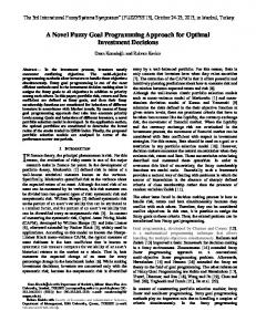
Quantitative Methods Inquires Linear membership functions are used in literature and practice more than other types of membership functions. For the above three types of fuzzy goals linear membership functions are defined and depicted as follows ( Fig. 1): Membership function

μZ

k

Analytical definition

( x)

1

μZ

gk

μZ

k

k

( x)

U k G k (x )

( x)

1

μZ

Lk

μZ

k

⎧1..................if ..G k ( x) ≤ g k ⎪ ⎪ u − G k ( x) ..if ..g k ≤ G k ( x) ≤ u k ...k = 1,..., m...(1) =⎨ k ⎪ uk − g k ⎪⎩0................if ..G k ( x ) ≥ g k

gk

k

( x)

⎧1..................if ..Gk ( x) ≥ g k ⎪ ⎪ G ( x) − Lk ..if ..Lk ≤ Gk ( x) ≤ g k ...k = m + 1,..., n....(2) =⎨ k ⎪ g k − Lk ⎪⎩0................if ..Gk ( x) ≤ Lk

G k (x)

( x)

1

μZ

Lk

gk

Uk

k

( x)

⎧0..................if ..Gk ( x) ≤ Lk ⎪ G ( x) − L k ⎪ k ..if ..Lk ≤ Gk ( x) ≤ g k ...k = n + 1,..., l ⎪ g k − Lk ....(3) =⎨ ⎪ uk − Gk ( x) ..if ...g ≤ G ( x) ≤ u k k k ⎪ uk − g k ⎪ ⎩0................if ..Gk ( x) ≥ uk

G k (x)

Figure 1. Linear membership function and Analytical definition Where L K (or u k ) is lower (upper) tolerance limit for k.th fuzzy goal G k ( x) They are either subjectively chosen by decision makers or tolerances in a technical process (Chen & Tsai, 2001; Yaghoobi & Tamiz, 2007). 2.3.2. FGPIP-APP formulation We will use the method that was developed by Chen & Tsai,( 2001 ) for formulated the APP problem in the fuzzy gaols , which allows decision makers to determine a desired achievement degree and importance (or weight) of each of the fuzzy goals, The complete FGPIP-APP model can be formulated as follows. l

Max.. f (u ) = ∑ μ k k =1

322

Quantitative Methods Inquires Subject to :

μ1 ≤ μ z

1

μ2 ≤ μ z

2

μ3 ≤ μ Z

3

(Minimize total production costs ). (Minimize carrying costs ). (Minimize changes in labor levels).

X it + I i ,t −1 − I it = d it I it ≥ I it .Min Wt − Wt −1 − H t + Ft = 0 WMin ≤ Wt ≤ WMax Pit − K it * Wt ≤ 0

μ1 ≤ α 1 μ2 ≤ α 2

μ3 ≤ α 3 Pit , I it ,Wt , H t , Ft ≥ 0 Where α 1 , α 2 , α 3 is the desirable achievement value for the i -th fuzzy goal. 2.3.3. Fuzzy linguistic for determing the degree of achievement The determination of a desirable achievement degree for a goal could be a difficult task for a DM in a fuzzy environment when using method by Chen & Tsai,( 2001 ) . For assessing desirable achievement degrees imprecisely, a useful method is to use linguistic terms such as ‘‘Low Important”, ‘‘Somewhat High Important”, and ‘‘Very High Important” and so on to verbally describe the importance of each fuzzy goal. the associated membership function are then defined. We can define

μ I (α ) to

represent the membership function of

each linguistic values about the importance of different objectives, where

α denotes

μ I (α ) ∈ [0,1] , and

the variable taking an achievement degree in the interval of

[α min .α max ],

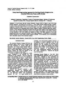
0 ≤ α min ≤ α max ≤ 1 Then fuzzy numbers ranking methods can be used to map a membership function representing a fuzzy goal’s importance to a real number in the range of [0,1]. The real number obtained can be considered as the desirable achievement degree for the fuzzy goal. We define I = {Very Low Important = VLI, Low Important = LI, Somewhat Low Important = SLI, Medium = M, Somewhat High Important = SHI, High Important = HI, Very High Important = VHI} as a set of linguistic values about the importance of different goals (FIG.2). shows the

μ I (α )

for this linguistic values. Triangular fuzzy numbers corresponding

to these linguistic values are: VLI = (0,0,10%), LI = (5%,15%,25%), SLI = (20%,32.5%, 45%), M = (40%, 50%,60%), SHI = (55%,67.5% ,80%), HI = (75%, 85%, 95%), VHI = (90%, 100%, 100%).

323


μ I (α ) 1 VLI

LI

SLI

M

SHI

HI

VHI

α 0

5

10

15 20

25 32,5 40

45 50

55

60 67,5 75

80 85 90

95 100

Figure 2. Membership functions for Linguistic values about the importance of different objectives Note that subject to definition of fuzzy number, a and d corresponds, respectively, to

α min and α max .

We use Liou and Wang (1992) approach for ranking fuzzy numbers to

precisely determining the degree of achievement of different goals. As stated earlier, in μ k

≥ α k the α k shows the degree of achievement of k th fuzzy goal. In Liou and Wang ~ (1992) method, given α ∈ [0,1] total integral value of triangular fuzzy number A = ( a, b, c ) is:

~ ~ I Tα = α .I R ( A) + (1 − α ).I L ( A)

∫

= α

∫0 [c

= R

1

= α

0 1

g

R ~ A

( y ) dy + (1 − α

)∫0

1

g

L ~ A

(y)

+ ( b − c ) y ]. dy + (1 − α

)∫0 [a 1

+ ( b − a ) y ]. dy .

1 [α .c + b + (1 − α ). a ] 2

L

Where g A~ , g A~ corresponding inverse functions the triangular membership function can be defined as :

⎧ ⎪ ⎪ ⎪ μ .( x ) = ⎨ ⎪ ⎪ ⎪ ⎩ •

0 .........

if .. x ≤ a

x − a .. if .. a ≤ x ≤ b b − a x − c .. if ... b ≤ x ≤ c b − c if .. x ≥ c 0 ........

~

when α = 0 , the total integral value I T ( A) which represents a pessimistic decision 0

maker’s the totale integrale value becomes :

1 ~ I T0 ( A) = [b + a ] 2 •

~

when α = 0.5 , the total integral value I T ( A) which represents a moderate decision 0.5

maker’s the totale integrale value becomes:

1 ~ I T0.5 ( A) = [0.5.c + b + 0.5.a ] 2

324

(percentage)

Quantitative Methods Inquires •

when α = 1 , the total integral value

~ I T1 ( A) which represents a optimistic decision

maker’s the totale integrale value becomes : ~ 1 I T1 ( A) = [c + b] 2

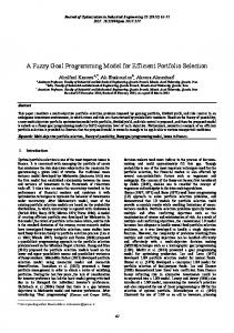
3. Model implementation 3.1. An industrial case study and data description In this section, as a real-world industrial case a data set provided by the national firm of iron manufactures non- metallic and useful substances (BENTAL) in Algeria , This company manufactures three types of products which are important, and one of the raw materials used in many industries with : Bentonite (BEN) , Carbonate of calcium (CAL) , Discoloring (TD), The Firm operates 175 workers, and the system of work in the Firm is a continuous production (8×3 hours) for all days of the week except Thursday hailed the work is only a half-day and Friday, which is rest day, and production management composed in 68 worker divide in 3 groups. The individual firm in the production of mineral products mentioned above, the demand for their products makes is large, which may cause problems in the productive capacity of this firm, fig.3 show fluctuations in demand on the level of monthly production capacity of any production capacity (CAP).

Figure 3. The fluctuation of the actual demand on the level of production capacity for TD, BEN, CAL Therefore, fluctuations in demand on the level and volatility of productive capacity, calls for the Firm in an attempt to develop a plan of production, trying to cope with the impact that fluctuations in demand due to seasonal changes, Table 1 summarizes the basic data gathered from the firm , The proposed model implementation in the company has the following conditions: 1. There is a Six period planning horizon. 2. A three product situation is considered. 3. The initial inventory in period 1 is I 10 and I 30

= 1857 Tons of BEN, I 20 = 1029 Tons of TD

= 1860 Tons of CAL.

4. Minimum inventory must be maintained during the period t of product i is 500.Tons 5. The costs associated with hiring and laying off, according to estimations of human resource management department per man are respectively 5178DA/man and 4155 DA/man. 6. The Linguistic values about the importance of objectives are : Very High Important = VHI, High Important = HI, Medium = M. respectively . and assumed that we have moderate decision maker , with

α = 0 .5 .

325

Quantitative Methods Inquires 7. The cost of one worker in the production of three products during the

t period is

rt = 2694.706.DA / man 8. The minimum work force level (man) available in each period is 9. The maximum work force level available in each period is 10. The initial worker level is ( W0

WMin = 55 worker .

WMax = 68 worker .

= 68 ).

11. the Maximum capacity of storage in 3 products in the firms is 6000 Tons. Table 1. The basic data provided by Bental firm (in units of Algerian Dinar DA ...1$ ≅ 90 DA) Product

BEN ( P1t )

TD

( P2t )

CAL

( P3t )

Period

d it

vit

cit

K it

1 2 3 4 5 6 1 2 3 4 5 6 1 2 3 4 5 6

1177.225 923.021 883.342 1071.99 1379.269 1315.222 128.620 163.777 164.617 166.005 193.317 206.662 1164.191 463.447 659.034 425.240 78.967 478.221

3293.493 3293.493 3293.493 3293.493 3293.493 3293.493 21646.608 21646.608 21646.608 21646.608 21646.608 21646.608 1296.109 1296.109 1296.109 1296.109 1296.109 1296.109

208.796 208.796 208.796 208.796 208.796 208.796 848.721 848.721 848.721 848.721 848.721 848.721 139.149 139.149 139.149 139.149 139.149 139.149

17.794 15.367 18.602 16.985 17.794 17.794 3.883 3.353 4.059 3.706 3.883 3.883 14.558 12.573 15.220 13.897 14.558 14.558

3.2. Formulate and solving problem by FGPIP-APP 3.2.1. Construct the membership functions The linear membership function of each objective function is determined by asking the DM to specify the interval

[g k ..u k ]

of the objective values, and also to specify the

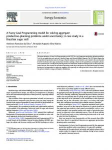
equivalence of these objective values as a membership value in the interval [0, 1]. The linear and continuous membership function is found to be suitable for quantifying the fuzzy spiration levels. The corresponding linear membership functions can be defined in accordance with analytical definition of membership functions (Fig.1 Eq (1) ). as follows.

μZ

1

1

⎧1.......... .......... .......... ..........if ...Z1 ≤ 32000000 ⎪ 33000000 − Z1 ⎪ μ Z1 ⎨ ......if ...32000000 ≤ Z1 ≤ 33000000 . ⎪ 33000000 − 320000000 ⎪⎩0.......... .......... .......... ........if ...Z1 ≥ 33000000 .

32000000 33000000 Z1 Figure 4. Membership function of Z 1 (Minimize total production costs)

326


μZ

2

⎧1.......... .......... .......... ..........if ...Z 2 ≤ 4350000 ⎪ 4600000 − Z ⎪ 2 μZ 2 ⎨ ......if ...4350000 ≤ Z 2 ≤ 4600000 . ⎪ 4350000 − 4600000 ⎩⎪0.......... .......... .......... ........if ...Z 2 ≥ 4600000 .

1

4350000 4600000

Z2

Figure 5. Membership function of Z 2 (Minimize carrying costs )

μZ

3

⎧1.......... .......... ......if ...Z 3 ≤ 0 ⎪13 − Z ⎪ 2 μZ3 ⎨ .......... ....if ...0 ≤ Z 3 ≤ 13. 13 ⎪ ⎪⎩0.......... .......... .....if ...Z 3 ≥ 13.

1

13 Z3

Figure 6. Membership function of Z 3 ( Minimize changes in labor levels) 3.2.2. Transform FGPIP-APP problem to linear programming(LP) Transform FGPIP-APP problem to equivalent LP with one objective that maximizes the summation of achievement degrees. The LP model for FGPP-APP problem is constructed as follows: 3

Max.. f (u ) = ∑ μ k k =1

Subject to :

μ1 ≤ (33000000 − Z 1 ) 1000000 . μ 2 ≤ (4400000 − Z 2 ) 250000 . μ 3 ≤ (13 − Z 3 ) 13.

Pit − K it × Wt ≤ 0 Pit + I i ,t −1 − I it = d it Wt − Wt −1 − H t + Ft = 0 WMin ≤ Wt ≤ WMax 3

∑I i =1

it

≤ 6000

I it ≥ 500

327


I 10 = 1856.25 I 20 = 1029 I 30 = 1860 W0 = 68

μ1 ≥ 0.725 μ 2 ≥ 0.850 μ 3 ≥ 0.50 Pit , I it ,Wt , H t , Ft , μ1 , μ 2 , μ 3 ≥ 0

i = 1.,2.,3

t = 1.,2.,......,6

Wt , H t , Ft (integers). 3.2.3. Solve the FGPIP-APP Problem The LINGO computer software package was used to run the Linear programming model. Table 2 presents the optimal aggregate production plan in the industrial case study based on the current information: Table 2. Optimal production plan in the BENTAL firm case with FGPIP-APP model Period 0

1

2

3

4

5

6

Product 1 (BEN) 2 (CAL) 3 (TD) 1 (BEN) 2 (CAL) 3 (TD) 1 (BEN) 2 (CAL) 3 (TD) 1 (BEN) 2 (CAL) 3 (TD) 1 (BEN) 2 (CAL) 3 (TD) 1 (BEN) 2 (CAL) 3 (TD) 1 (BEN) 2 (CAL) 3 (TD)

Pit

I it

Wt

Ht

Ft

(Tons) 0 0 0 743.996 0 267.638 1074.857 0 659.034 1154.980 94.019 425.24 1209.992 193.317 78.967 1209.992 206.662 478.221

(Tons) 1865.25 1029 1860 679.025 900.38 695.809 500 736.603 500 691.515 571.986 500 774.505 500 500 605.228 500 500 500 500 500

(man) 68

(man) -

(man) -

68

0

0

68

0

0

68

0

0

68

0

0

68

0

0

68

0

0

Using FGPIP to simultaneously minimize total production costs ( Z 1 ), carrying costs ( Z 2 ), and changes in Work force levels ( Z 3 ), yields total production cost of 32032504.2 DA, carrying cost of

4375292.99 DA, and changes in Work force levels of 0. and resulting

achievement degrees for the three fuzzy goal ( μ1 ,

μ2

and μ 3 ) are 0.9682679 ,

0.8975380 and 1 respectively , all of which satisfy the requirements of decision makers.

328

Quantitative Methods Inquires Despite the good results that were obtained through the proposed model , but remains very much sensitive to the accuracy of the information and data provided by the Organization,

4. Conclusions: The APP is concerned with the determination of production, the inventory and the workforce levels of a company on a finite time horizon. The objective is to reduce the total overall cost to fulfill a no constant demand assuming fixed sale and production capacity. In this study we proposed an application of a fuzzy goal programming approach with different importance and priorities developed by Chen and Tsai (2001) to aggregate production planning, The proposed model attempts to minimize total production and work force costs, carrying inventory costs and rates of changes in Work force so that in the end, the proposed models is solved by using LINGO program and getting optimal production plan. The major limitations of the proposed model concern the assumptions made in determining each of the decision parameters, with reference to production costs, forecasted demand, maximum work force levels,, and production resources. Hence, the proposed model must be modified to make it better suited to practical applications. Future researchers may also explore the fuzzy properties of decision variables, coefficients, and relevant decision parameters in APP decision problems.

References 1. 2. 3. 4. 5. 6. 7. 8. 9. 10. 11. 12. 13.

Bowman, E. H. Consistency and optimality in managerial decision making, Management Science, 9, 1963, pp. 310–321 Bowman, E. H. Production scheduling by the transportation method of linear programming, Operations Research, 4, 1956, pp. 100–103 Charnes, A. and Cooper, W.W. Management models and industrial applications of linear programming, Wiley, New York, 1961 Chen, L.H. and Tsai, F.C. Fuzzy goal programming with different importance and priorities, European Journal of Operational Research, 133, 2001, pp. 548–556 Hannan, E.L . On Fuzzy Goal Programming, Decision Sciences 12, 1981-b, pp. 522–531 Hannan, E.L. Linear programming with multiple fuzzy goals, Fuzzy Sets and Systems, 6, 1981-a, pp. 235-248 Holt, C.C., Modigliani, F and Simon, H.A. Linear decision rule for production and employment scheduling, Management Science 2, 1955, pp. 1–30 Jamalnia, A. and Soukhakian, M.A. A hybrid fuzzy goal with different goal priorities to aggregate production planning, 2008, pp. 1-13 Jones, C. H. Parametric production planning, Management Science, 13, 1967, pp. 843–866 Leberling, H. On finding compromise solutions in multi criteria problems using the fuzzy min-operator, Fuzzy Sets and Systems, 6, 1981, pp. 105–118 Lee, Y.Y. Fuzzy set theory approach to aggregate production planning and inventory control, PhD Dissertation, Department of I.E., Kansas State University, 1990 Liou, T. S. and Wang, M.T. Ranking fuzzy numbers with integral value, Fuzzy Sets and Systems, 50, 1992, pp. 247–255 Luhandjula, M. K. Compensatory operations in fuzzy programming with multiple objectives, Fuzzy Sets and Systems, 8, 1982, pp. 245–252

329

Quantitative Methods Inquires 14. Masud, A. S. M. and Hwang, C. L. An aggregate production planning model and application of three multiple objective decision methods, International Journal of Production Research, 18, 1980, pp. 741–752 15. Narasimhan, R. Goal Programming in a Fuzzy Environment, Decision Sciences, 11, 1980, pp. 325–336 16. Rubin, P. A. and Narasimhan, R. Fuzzy goal programming with nested priorities, Fuzzy Sets and Systems, 14, 1984, pp. 115–129 17. Saad, C. An overview of production planning model: structure classification and empirical assessment, Int. J. Prod. Res., 20, 1982, pp. 105–114 18. Sakawa, M. An interactive fuzzy satisficing method for multi objective linear fractional programming problems, Fuzzy Sets and Systems, 28, 1988, pp. 129–144 19. Sakawa, M. and Yauchi, K. An interactive fuzzy satisficing method for multi objective nonconvex programming problems with fuzzy numbers through coevolutionary genetic algorithms, IEEE Transactions on Systems, Man. and Cybernetics – Part B, 31(3), 2001, pp. 459–467 20. Singhal, K. and Adlakha, V. Cost and shortage trade-offs in aggregate production planning, Decision Sciences, 20, 1989, pp. 158–165 21. Tang, J., Wang, D., and Fung, R. Y. K. Fuzzy formulation for multi-product aggregate production planning, Production Planning and Control, 11, 2000, pp. 670–676 22. Taubert, W. H. A search decision rule for the aggregate scheduling problem, Management Science, l4, 1968, pp. 343–359 23. Tiwari, R. N., Dharmar, S., and Rao, J. R. Fuzzy goal programming – An additive model, Fuzzy Sets and Systems, 24, 1987, pp. 27–34 24. Wang, H. F. and Fu, C. C. A generalization of fuzzy goal programming with preemptive structure, Computers and Operations Research, 24, 1997, pp. 819–828 25. Wang, R. C. and Fang, H. H. Aggregate production planning with multiple objectives in a fuzzy environment, European Journal of Operational Research, 133, 2001, pp. 521– 536 26. Wang, R.-C. and Liang, T.-F. Aggregate production planning with multiple fuzzy goals, International Journal of Advanced Manufacturing Technology ,Vol 25, 2005, pp. 589– 597 27. Wang, R.-C. and Liang, T.-F. Application of fuzzy multi-objective linear programming to aggregate production planning, Computers and Industrial Engineering, 46, 2004, pp. 17–41 28. Yaghoobi, M. A. and Tamiz, M. A method for solving fuzzy goal programming problems based on MINMAX approach, European Journal of Operational Research, 177, 2007, pp. 1580–1590 29. Zadeh, L. A. Fuzzy Sets, Information and Control, 8, 1965, pp. 338–353 30. Zimmermann, H. J. Applications of fuzzy sets theory to mathematical programming, Information Science, 35, 1985, pp. 29-58 31. Zimmermann, H.-J. Description and optimization of fuzzy systems, International Journal of General Systems, 2, 1976, pp. 209–215 32. Zimmermen, H. J. Fuzzy programming and linear programming with several objective functions, Fuzzy Sets and Systems, 1, 1978, pp. 45–56

1

Mostefa Belmokaddem, Doctor of Economics, University professor - was graduate of the Faculty of Economics at the University of Oran in 1977 and worked as assistant lecturer and professor at the Faculty of Economics University of Tlemcen (Algeria). After receiving his Ph.D. (1982)in the Theoretical Statistics and Economics at the Academy of Economic Studies in Bucharest, he worked as a Lecturer at the Faculty of Economics, University of Tlemcen, Algeria, (1982-1989 ), Lecturer (1988-1990) and professor (1990 to present). He has participated in international scientific events and a

330


summer school (Valencia, Spain). It presents his ideas on a wide band of key issues in microeconomics, the various techniques to aid decision making by providing useful information for each discipline and research projects. He is the author of handouts and has published several articles in journals. The subjects are currently being microeconomics, applied microeconomics, econometrics and applied econometrics, applied statistics and goal programming (undergraduate, PhD School of Economics). 2 Mékidiche Mohammed is currently Assistant Professor in the faculty of economics and commerce , University of Tlemcen, Maghnia Annex, Algeria , where he teaches Statistics and Operations Research He received the MS degree in production and operations Management at Faculty of Economics and commerce , University of Tlemcen,Algeria in 2005 . Mékidiche Mohammed is currently a PhD candidate in the field of production and operations Management at University of Tlemcen . His research project is optimization in production planning, fuzzy optimization and its application in production planning and scheduling, Time series analysis and its application in forecasting, neural network and its application in management. 3

SAHED Abelkader holds a Masters degree in production and operations Management from Tlemcen University (2006), is currently a PhD candidate in the field of production and operations Management at University of Tlemcen. He teaches courses in statistics, probability, and Econometrics. His research interests include decision making, goal programming, fuzzy sets, decision making, operation and production management, and Econometrics.

331