Application of neural networks in process engineering

Application of neural networks in process engineering: simulation and online implementation Brink, A

22782109

Janse van Rensburg, F

22812415

Meyer, A

22840176

Simpson, Q

22833005

Group 7 – Assignment 1

North-West University CEMI 414 Frikkie van der Merwe

11/4/2014

Executive Summary As an application to chemical and process engineering neural networks has been implemented in order to predict sensor data and other applications such as fault detection and recently nonlinear applications in process control in the form of inference control. This paper intends to simulate the neural network control on both simulation and online for a CSTR equipped with a cooling jacket, and a pressure temperature control process of an ideal gas online respectively. For this specific neural network a thee layer system was implemented, of which the input layer consists of three input neurons, the hidden layer consists of two neurons and one output neuron. The neural network used for this study trains rapidly, with a small error accompanied by a remarkable data regression. For a linear process the prediction could handle extrapolation sufficiently however, for a strong nonlinear process the extrapolation did not predict adequately.

i

Table of Contents Executive Summary ............................................................................................................... i List of Figures ....................................................................................................................... iii List of Tables ........................................................................................................................iv 1

Introduction .................................................................................................................... 1

2

Artificial neural networks ................................................................................................ 2 2.1

Back propagation algorithm .................................................................................... 2

2.2

Neural networks architectures ................................................................................. 4

2.2.1

Feed forward networks .................................................................................... 5

2.2.2

Recurrent networks .......................................................................................... 5

2.3

Types of artificial neural networks ........................................................................... 6

i)

Multilayer Perceptron .............................................................................................. 6

ii)

Radial Basis Function Networks.............................................................................. 7

iii)

Kohonen Neural Network .................................................................................... 8

2.4

Mathematical Model .............................................................................................. 10

2.5

Learning methods ................................................................................................. 11

2.6

Applications .......................................................................................................... 12

2.6.1 2.7 3

Process Control ............................................................................................. 12

Characteristics ...................................................................................................... 18

Demonstration of Neural Network ................................................................................ 19 3.1

Topography........................................................................................................... 19

3.2

[1] The CSTR ........................................................................................................ 20

3.3

[2] Pressure Temperature System: ....................................................................... 27

4

Critical evaluation......................................................................................................... 33

5

Bibliography ................................................................................................................. 35 User Manuel of the neural network .................................................................................A-1 Source Code ..................................................................................................................B-2

ii

List of Figures Figure 2.1: A single neuron ................................................................................................... 2 Figure 2.2: A multi-layer feed forward neural network ........................................................... 5 Figure 2.3: A multi-layer feed forward neural network ........................................................... 6 Figure 2.4: Feed forward multilayer developing structure ...................................................... 7 Figure 2.5: Radial Basis Function ......................................................................................... 8 Figure 2.6: Growing Neural Gas ............................................................................................ 9 Figure 2.7: Various Neural Networks................................................................................... 10 Figure 2.8: Mathematical representation of Neural Networks .............................................. 10 Figure 2.9: Neural networks in indirect adaptive strategy .................................................... 13 Figure 2.10: Model predictive control .................................................................................. 14 Figure 2.11: Neural networks in internal-model-control strategy .......................................... 15 Figure 2.12: Stabalizing controller ....................................................................................... 16 Figure 2.13: Non-linear internal model control ..................................................................... 16 Figure 2.14: Model predictive control .................................................................................. 17 Figure 2.15: Adaptive critic .................................................................................................. 17 Figure 3.1: Structure of the neural network used ................................................................. 19 Figure 3.2: Concentration vs. time graph............................................................................. 21 Figure 3.3: Comparison of data obtained vs. predicted data................................................ 22 Figure 3.4: Regression fit .................................................................................................... 23 Figure 3.5: Weights calculated for first 119 data sets .......................................................... 23 Figure 3.6: Untrained regression data ................................................................................. 24 Figure 3.7: Graph after training the second set of data........................................................ 25 Figure 3.8: Full range data set vs. predicted values ............................................................ 26 Figure 3.9: HYSES simulation of a pressure/temperature system ....................................... 27 Figure 3.10 : First case after training has been done on the pressure temperature data. .... 28 Figure 3.11 : Case 2 after no-training has been done on the new pressure /temperature data. ........................................................................................................................................... 29 Figure 3.12 : Case 3 after no –training on the new pressure/temperature data. .................. 30 Figure 3.13: Case 4 after no –training on the new pressure/temperature data .................... 31 Figure 3.14 : Case 4 data after training on the pressure/temperature data. ......................... 32

iii

List of Tables Table 2.1: Attributions of multilayer perceptron’s ................................................................... 7 Table 2.2: Attributions of radial basis function networks ........................................................ 8 Table 2.3: Kohonen neural network aplications ..................................................................... 9 Table 2.4: Characteristics of Neural Networks .................................................................... 18 Table 2.5: Advantages and Disadvantages for various neural network structures ............... 18 Table 3.1: Input and output variables .................................................................................. 20

iv

1 Introduction Recently an active development in the application of nonlinear control methodologies have received much interest lodging an imperative position in process control engineering, seen by an increasing amount of research papers being published in open literature. This being said it is still extremely difficult to implement control methods in some applications from first principles. This led to various nonlinear models being developed for certain regions in process control. One of the main obstacles in the current implementation of nonlinear control applications is the high cost of constricting and validating the model, especially in the chemical/petroleum industry. The upsurge in neural networks used to control nonlinear processes offers an alternative less expensive method to other nonlinear control methods. Neural networks can learn by example, making it more proficient than current control methods, and it is due to this that it is much more cost-efficient. Although the application of neural networks has been implemented in general engineering for quite some time, only recently has it emerged in process control engineering. This can be attributed to: i.

Recent advances in digital technology have made neural network simulations a cost effective way of controlling chemical units. Also advances computational speeds made simulations a viable option.

ii.

The superiority of the neural network to conventional controlling methods in terms of its wider range of applicability and robustness.

iii.

In some cases neural networks can be easier to apply to a process

Neural networks have been widely applied to chemical engineering, but only recently has it been applied to process control procedures. The majority of these neural networks were of a multilayer feed forward structure (Hussain, 1999). The applications employing these neural networks in the chemical engineering industry range from the most linear processes (flash drum) to some of the most complex nonlinear processes (exothermal CSTR). The most common process units employing neural networks are distillation columns and reactor systems (continuous stirred tank reactors) In this paper only one neural network was used with three inputs, two hidden neurons and one output neuron.

1

2 Artificial neural networks In accordance with Jain et al. (1996) artificial neural networks are scientific developing systems, inspired by biological neural networks and inherit the learning and reasoning properties seen in human brains. Recently research in designing artificial neural networks have spiked in multidisciplinary areas to solve a variety of problems in pattern recondition, associative memory, optimizing, prediction and control applications. Although successful and intelligent applications have been developed in constrained environments, few are flexible enough to perform outside its domain. Artificial neural networks provide exiting alternatives from which many applications could benefit from. A neural network subsists of a set of connected cells; neurons, which receive impulses from either input cells or other neurons depending on the arrangement of the model. Producing some sort of transformation in the input cells or other neurons transmitting the result to either other neurons or the output sells (Jha, 2011). The neural network is constructed in such a manner that the neurons are connected to the other neuron layers that receives the input from the preceding layer and passes the output to the subsequent layer. A schematic representation of neuron is depicting in Figure 2.1

Figure 2.1: A single neuron

2.1 Back propagation algorithm This back propagation algorithm is used in layered artificial neural networks meaning that artificial neurons send their signals forward and errors are transmitted in epoch. The first segment of layers receives input values from neurons followed by an output for the neural network.

2

Hidden layer amounts are dependent on the type of transform function. In order for the back propagation algorithm to calculate the errors1, inputs and outputs must be fed to the system. Back propagation algorithms are used to reduce these errors until the artificial neural networks are trained. The training comprises taking random weights at the beginning and then adjusting these weights until the error is minimal. The activation function (depended on the weights and inputs) is calculated with the following equation: ( ̅ ̅) Where

∑

2.1

resembles the inputs and

their respective weights.

The following equation is used to calculate a sigmoidal function: ( ̅ ̅)

( ̅ ̅)

2.2

For large positive and negative numbers the sigmoidal function will approach 1 and 0 respectively. For an activation number of 0 the sigmoidal function will reach 0.5, resulting in smooth transitions between high and low neuron outputs. The goal of the algorithm is to obtain an output value desired for the training process. The simplified error function for all the neuron outputs can be defined as: ( ̅ ̅

̅)

∑( ( ̅ ̅)

)

2.3

The back propagation algorithm calculates the error’s dependence on the input, output and the weights. After the dependence is calculated, the weights can be calculated by using the gradient descendent method:

2.4

The adjustment size will depend on η2 and on the weights contribution to the error, which relates to a larger adjustment when the contribution of the weight to the error is large. Equation 2.4 is used to find weights that minimalize the error.

1 2

The error is calculated from the difference between expected and actual results. Constant

3

The dependency of the error on the output can be related to: (

)

2.5

Followed by the output’s dependence on the activation: (

)

2.6

Combining equations 2.5;6 gives the dependency of the error on the activation: (

) (

)

2.7

Combining equations 2.7 and 2.4 gives each weights adjustment for the training of a two layer artificial neural network: (

) (

)

2.8

When a third order system is considered the errors dependency is calculated from the input of the previous layer 2.9

where

is defined as adjustment of weights from a previous layer where: (

) (

2.10

)

Finally for a three layer system assuming there are inputs to

in the form of

the

following equation is obtained: (

)

2.11

REMARK: It is important to consider the exponential increase in training times when extra layers are considered for the back propagation method, if no additional data is supplied. Refinements are also available for faster back propagation learning. Source: (Gershenson, 2014)

2.2 Neural networks architectures There are several types of artificial neural networks, but the most common and widely used neural networks are discussed in the preceding sections.

4

2.2.1

Feed forward networks

In a feed forward network, information flows in one direction; forward, along the connecting pathways, from the input layers along the hidden layers to the output layers. There exists no feedback loops, thus resulting in a straight flow of information, with the subsequent layers not influencing the preceding layers. Figure 2.2 is a representation of a multi-layer feed forward neural network

Figure 2.2: A multi-layer feed forward neural network

2.2.2

Recurrent networks

Differences between these type of networks and feed forward networks are that recurrent networks uses at least one epoch. There could be neurons with self-feedback links, thus the output of the neuron is fed back into itself as input.

5

Figure 2.3: A multi-layer feed forward neural network

Source: (Elman, 1991)

2.3 Types of artificial neural networks The most important and applicable class of neural network architecture for real world problems solving includes:  Multilayer Precipitation  Radial Basis Function Networks  Kohonen Self Organizing Feature Maps i)

Multilayer Perceptron The most common and popular form of neural networks architecture is the multilayer perceptron. Multilayer perceptron’s are feed-forward networks with at least one hidden layer. One of the critical features in multilayer perceptron’s in the non-linearity at the hidden layer, otherwise the multilayer perceptron could have been replaced by a single layer of perceptron’s. Table 2.1 states some of the attributes and features of multilayer perceptron:

6

Table 2.1: Attributions of multilayer perceptron’s

Is not dependent on the amount of inputs At the input layers the use of linear combination functions are utilized Has at least one hidden layer independent of the unit amount Generally uses sigmoid activation functions in hidden layers Has any number of outputs not dependent of the activation function Has connection between input layers and first hidden layer, with subsequently connection between hidden layers until the last hidden layer which in connected with the output layer. A change in the input weight to a hidden neuron indirectly effects the output weights from the hidden layer Source: (Hebb, 1949) According to Hebb (1949) multilayer perceptron’s with enough given data, hidden neurons and training time, could learn to approximate effectively any function to any degree of accuracy, resulting in the use of these designs for processes where you have little prior knowledge of the relationship of the units. If there is a system with more than one hidden layer, much less data have to be given to the hidden layers in order for the weight to be calculated, resulting in improvements in generalization.

Figure 2.4: Feed forward multilayer developing structure

ii)

Radial Basis Function Networks

Another feed forward network is a radial basis function, these networks however only has one hidden layer. Some attributes and features of such networks are:

7

Table 2.2: Attributions of radial basis function networks

Source: (Jha, 2011)

Figure 2.5: Radial Basis Function

iii)

Kohonen Neural Network

In contrast to the other two networks mentioned in the previous discussions, the kohonen neural network is not designed for supervised learning tasks, but rather primarily unsupervised learning (Patterson, 1996). According to Patterson (1996) this type of network attempts to learn the tendency of the data structure rather than to manipulate weights in order to achieve a certain output. This method tends to recognise deviations in the training data and responds accordingly, however if new data is included, unlike the previous data, the network system fails to respond to the new training data signifying novelty to the network. A kohonen network only has two layers: the input and output layers In the case of a growing neural gas in Fritzke (1995) the network adapts to a signal distribution that has vastly varying dimensions in other areas of the input space as shown in Figure 2.6.

8

Figure 2.6: Growing Neural Gas

As can be seen in Figure 2.6, the neural network adapts to the signal disturbances accordingly. Table 2.3: Kohonen neural network aplications

Process Control

Feed forward control, seeing that the networks main attribute is reading the data tendency

Financial

Used to forecast financial and economic time series

Agricultural

Forecasting plant diseases growth rate

Source: (Fritzke, 1995) In all there are many applications of the kohonen neural network, ranging from agriculture to zoology; most of these applications are however feed forward applications. The feed forward networks and the looping networks can be classified as in Figure 2.7.

9

Figure 2.7: Various Neural Networks

Source: (Jain et al., 1996)

2.4 Mathematical Model

Figure 2.8: Mathematical representation of Neural Networks

Source: (Dorofki et al., 2012) The mathematical model in Figure 2.8 consists out of synapses and is weighted. In mathematical terms the neuron could be represented by:

∑

2.12

And the output ( ) represented by:

10

(

)

2.13

The adaptation of the weight vector is given as follows: (

)

( )

( ( )

( )) ( )

2.14

Where ( ) is the desired output and ( ) is the activation value .New weight vectors are continuously being calculated until the error reached a minimum, therefore when

( )

( )

2.5 Learning methods Learning categories proposed by Awodele & Jegede (2009) is as follows: I.

Supervised learning : This type of learning integrates an external teaching source, evaluating the output to then give the appropriate response to change the input value accordingly.

II.

Unsupervised learning: This type of learning category only operates on the local information available to it, no external teaching is present. Internal data is being self-organised and detects the developing property.

Another proposed category by Jain (1996): III.

Hybrid learning : This fundamentally combines both supervised and unsupervised. Typically certain weights are being calculated as in the supervised method, whereas the other weights are being calculated in the unsupervised method.

IV.

Learning rate: When using a log-sigmoid and the learning rate is greater than 1, a more aggressive learning rate is witnessed, resulting in poor data regression (see Figure 3.4).

11

2.6 Applications 2.6.1

Process Control

These days the application of process engineering and process design under which the following falls:  Process supervision  Control  Estimation  Process fault detection and diagnosis rely on the effective processing of data which is unpredictable and imprecise. According to Hussain (1999), neural networks have mainly been implimented in applications such as sensor data analysis and fault detection. Later it also indicated nonlinear processes being predicted by neural networks. However, reasently it has been used in process control ranging over a wide range of control applications. The use of feed forward control has been recieving much attention these days as mentioned in Table 2.3. Neuron networks have been implimented due to its accuracity, ease of use and implimentation on nonlinear functions compared to mathematical application in the process engineering industry. Psichogios & Ungar (1991) employed a neural network model to control the product concentration of a CSTR while making use of a multylayer perceptron sigmoid neural network. 2.6.1.1 Neural networks in adaptive control techniques 2.6.1.1.1 General description Neural networks can be adapted into this technique3, to control non-linear dynamic systems. These adaptive network methods can be categorized as direct and indirect adaptive schemes. Direct adaptive – there is no direct attempt to determine the model of the system. The tendency of the data is tracked online; a direct result of the controller parameters being manipulated on-line. The algorithm causing the manipulation of the controller parameters can be based on gradient descent4

3 4

Conventional adaptive control structures Gradient descent – a form of backpropagation

12

Indirect adaptive – a neural; network is used to recognize an unknown function of a nonlinear plant online, refer to Error! Reference source not found.. the main purpose of this control strategy is to let the plant output follow a reference output initiated once the plant is identified to the desired level of accuracy. 2.6.1.1.2 Applications in chemical process systems Most of the literature made use of a cascade of two single hidden layers, radial basis function networks and the fuzzy logic systems (Ydstie, 1990); (Boslovic & Narendra, 1995); (Chovan et al., 1996); (Loh et al., 1995).

Figure 2.9: Neural networks in indirect adaptive strategy

Source: (Hussain, 1999) 2.6.1.2 Neural networks applied to model predictive control 2.6.1.2.1 General description A neural network used as a model predictive control is one of the most abundantly used control technique. In this technique the controller determines a variable profile that optimizes the open-loop performance objective in an undefined time interval while minimizing the future deviance outputs (see Figure 2.10)

13

Figure 2.10: Model predictive control

Source: (Hussain, 1999) 2.6.1.2.2 Applications in chemical process systems In most open literature set in Hussain (1999:58) a CSTR was controlled wile set point tacking. Most of the literature in Hagan & Demuth (1999:58) utelized the dynamic matrix control method, with cascade control being used. 2.6.1.3 Neural networks in inverse-model based techniques 2.6.1.3.1 General description Two approaches in the neural network in the inverse-mode-base strategy exist; [1] direct inverse control technique and [2] internal-model control technique. Direct inverse control technique – the inverse model performs as a controller in cascade; with the system that is under control. Thus the neural network acts as the controller, which has to learn to supply its output to the appropriate control parameters. The set point required acts as the output Internal model control – This method is much more robust than the previous mentioned. There are two main differences between the this method and the previous one mentioned, the first is the addition of a forward model placed in parallel with the plant. Secondly the error between the plant output and the neural network forward model is subtracted from the set point prior to being fed to the inverse model.

14

2.6.1.3.2 Application to chemical process systems Psichogios & Ungar, (1991) utilized the internal model control system to control the product concentration of a non-isothermal CSTR with first order reversible reactions. This was done by manipulating the inlet feed temperature. See Figure 2.11 for a scematic representation of the internal-model-control strategy as in (Hussain, 1999).

Figure 2.11: Neural networks in internal-model-control strategy

Source: (Hussain, 1999) 2.6.1.4 Online applications of neural network-based control strategies The majority online applications in open literature (Van Can et al., 1995); (Langonet, 1993); (Sheppard et al., 1992); (Baratt et al., 1995) utilizes the multi-layered feed forward network, whilst a few other use the recurrent and state feedback networks (Hussain, 1999). 2.6.1.5 Other applications 2.6.1.5.1 Fixed stabilizing controllers From Figure 2.12 it becomes evident that the model uses the desired trajectory as the input and the feedback control as an error signal. As the neuron network proceeds with the learnig process, in becomes evident that the input will converge to zero, resulting in the takeover of the neuron networks controller from the feedback controller (Hagan & Demuth, 1999). 15

Figure 2.12: Stabilizing controller

Source: (Hagan & Demuth, 1999) 2.6.1.5.2 Non-linear internal model control According to Hagan & Demuth (1999) the nonlinear control internal model control method consists of a neural network controller, plant model and robustness filter with a single tuning parameter, with the controller (neural network controller) is trained to represent the inverse of the plant. One major advantage of this method is that is can be trained offline, while using plant-data (Hagan & Demuth, 1999). Figure 2.13 is taken from (Hagan & Demuth, 1999)

Figure 2.13: Non-linear internal model control

Source: (Hagan & Demuth, 1999) 2.6.1.5.3 Model predictive control Model predictive Control optimizes the response of a plant over a specified certain time horizon. This optimization can be very expensive; requiring a multi-step ahead of calculation. In this step the neural network predicts the plant response; teaching the controller to produce the input selected by the optimization process. The model predictive control is represented by Figure 2.14.

16

Figure 2.14: Model predictive control

Source: (Hagan & Demuth, 1999) 2.6.1.5.4 Adaptive critic This control method consists of two neural networks; [1] operates the inverse controller (Action network) and [2] Critic network, which is trained to optimize future performance. Figure 2.15 shows the schematics of an adaptive critic controller as in (Hagan & Demuth, 1999)

Figure 2.15: Adaptive critic

Source: (Hagan & Demuth, 1999)

17

2.7 Characteristics Table 2.4: Characteristics of Neural Networks

Neural networks exhibit mapping capabilities; they are able to map certain input patterns and corroborate them with the associated output patterns Neural networks structural design can be ―trained‖ with known instances. This is normally done prior to testing for their ―inference‖ capabilities with of data with unknown instances. Has the capability of predicting new outcomes from past trends. Neural networks are robust systems which is fault tolerant Neural networks can process information at high speed, accurately, in parallel and in a distributed manner. Source: (Jha, 2011:41)

Table 2.5: Advantages and Disadvantages for various neural network structures

Advantages

Disadvantages

Linear Slower learning rate compared to others

Sometimes inaccurate Can only run linear data

Sigmoid Logistic Easy to differentiate

Delayed output

Accurate Predicting runoff data is plausible Exponential

Tangent Rapid

Difficult to differentiate

Chonic Inaccurate Sources: (Gardner & Dorling, 1997); (Thiria et al., 1993); (Dorofki et al., 2012); (Hayati & Shirvany, 2007); (Karlik, 2009)

18

3 Demonstration of Neural Network This section includes designed neural network demonstration. The section shows the neural network training on two different types of processes; [1] the training was a CSTR with cooling jacket and [2] a pressure-temperature system, to show the credibility of the network.

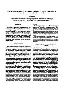
3.1 Topography The topography for the neural network during this project had three layers of which one was the input layer, the second the hidden layer and finally the being the output layer, whilst expending a log-sigmoid transfer function. The names as in Figure 3.1 are as mentioned in the accompanied program.

Figure 3.1: Structure of the neural network used

19

3.2 [1] The CSTR The CSTR model was modelled using the following equations.

3.1

3.2

3.3

3.4

As the network requires 3 input values and 1 output to train the network appropriately Table 3.1 gives the selected as inputs. Table 3.1: Input and output variables

Input

Variable

Unit

Input 1

Time

Seconds

Input 2

Temperature

Kelvin

Input 3

Temperature difference

Kelvin

Output

Concentration

Molar

20

With all the available data given the concentration-time curve is represented by Figure 3.2.

Figure 3.2: Concentration vs. time graph

Seeing that the designed neural network only works with 119 data sets at a specific time the first 119 data sets gave the following learning weights and output graphs. Figures of the graphs will be given in intervals due to the program running in intervals. It is important to note that the graphs will be labelled as trained or untrained the untrained graph which will relate to the previous weights calculated thus the untrained graphs will give insight to the capability of the network to extrapolate. First data given was from 0 seconds to 119 seconds. The following graphs (see Figures 3.3 and 3.4) were obtained after training the neural network.

21

Figure 3.3: Comparison of data obtained vs. predicted data

The following graph shows the real data vs. the predicted data. This was done in order to obtain a regression line and to see how well the data fits. The optimum regression line equation will be y=x with a R2 of 0.999.

22

Figure 3.4: Regression fit

It can be easily seen that the data fits extremely well while within the given data. Further the weight for the first 119 sets of data was determined by the network as.

Wout1 Wout2 W11 W12 W21 W22 W31 W32 -7.35657793 6.888151 3.666895 -1.37821 2.182982 2.446934 -3.99329 1.317124 Figure 3.5: Weights calculated for first 119 data sets

The next graph (see Figure 3.6) shows the next 119 data set with the previous weights calculated and it can clearly be seen that the data does not fit thus there is a problem with extrapolating the data for the first set when the input values are not within the trained data set’s range.

23

Figure 3.6: Untrained regression data

However after training the data given the new weight were calculated to be as follows.

24

Figure 3.7: Graph after training the second set of data

Thus this specific neural network can train for a certain amount of data, but lacks the ability to extrapolate this specific process. The following graph shows the training of the full data set to see if a proper prediction can be made through a bigger range of data sets after the network has completed its learning time.

25

Figure 3.8: Full range data set vs. predicted values

From the above curve it can be seen that network does have some degree of accuracy but battles to predict the initial points. The weights were found to be:

Wout1 Wout2 W11 W12 W21 W22 1.901171727 -5.44423 -0.46163 -2.00202 3.853835 4.453282

W31

W32 0

0

For this specific set only two inputs were selected. Thus explaining the weights being zero from the third input neuron.

26

3.3 [2] Pressure Temperature System:

Figure 3.9: HYSES simulation of a pressure/temperature system

In HYSES® a single stream was created containing nitrogen at 25°C .Two transfer functions were connected to the stream that gives noise on the pressure and temperature of the system as seen in Figure 3.9. TRF-1 manipulates the temperature and TRF-2 the pressure of stream 1. As a result of the pressure/temperature noise the molar volume changed with time typically accordingly to: (3.5) Assume ideal gas behaviour due to Nitrogen’s ideal behaviour at 25°C. For the first case the amplitude of sine wave used in TRF-1 and TRF-2 was 3% and 5% respectively. In the dynamic mode the strip chart and historical data was collected from the data book function. The pressure, temperature and molar volume data was then copied from the historical data to the neural network program in excel. For the first case the program was trained to calculate the appropriate weight vectors. Note that the y-axis ranges from 0 – 30 for Case 1, 2, 3 and 4 Case 1: TRF-1: 3% amplitude TRF-2: 5% amplitude Input 1: Temperature in Kelvin Input 2: Pressure kilo Pascal 27

Output: Molar Volume in cum/kgmole The graphical illustration after training has been done for the first case (see Figure 3.10):

Figure 3.10 : First case after training has been done on the pressure temperature data.

From Figure 3.10, it can be seen that the appropriate weight vectors has been calculated, due to the sequence of the lines being relatively the same. The blue line represents the trained line and the red line the actual data. To measure the capability of these calculated weight vectors to extrapolate we designed new cases for the test. For Case 2 and 3 the parameters of the transfer functions was changed to see how well the weights calculated in the first case fairs while extrapolating. Case 2: TRF-1: 8% amplitude TRF-2: 8% amplitude Input 1: Temperature in Kelvin Input 2: Pressure kilo Pascal Output: Molar Volume in cum/kgmole

28

Graphical illustration with no- training for case 2:

Figure 3.11 : Case 2 after no-training has been done on the new pressure /temperature data.

From Figure 3.11 it can be seen that with the original weights calculated the trend still follows the actual trend, the actual values and calculated values corresponds with a minor error present. Therefore the original calculated weights for Case 1 accurately predicted the values for Case 2. For Case 3 the amplitude is increased again of the transfer functions to see if the original calculated weights could still predict and extrapolate. Case 3: TRF-1: 20% amplitude TRF-2: 20% amplitude Input 1: Temperature in Kelvin Input 2: Pressure kilo Pascal Output: Molar Volume in cum/kgmole

29

Graphical illustration with no- training for case 3:

Figure 3.12 : Case 3 after no –training on the new pressure/temperature data.

From Figure 3.12 it can be concluded that the initial calculated weights form case 1, begins to reach the limits of the extrapolation and prediction capabilities. The actual values and calculated values start to differ significantly. Therefore the original calculated weights for case 1 could not be used to extrapolate data for case 3. In Case 4, the initial calculated weights for case 1 are still used. The sine wave generator on TRF-1 was not used; instead the noise function was used. For TRF-2 the original sine wave function was still used. It also important to note that for Case 4 the original calculated weights in Case 1 is used to see what the extrapolation potential of those weights are. Case 4: TRF-1: 5% (Noise) TRF-2: 8 % (Sine wave) Input 1: Temperature in Kelvin Input 2: Pressure kilo Pascal Output: Molar Volume in cum/kgmole

30

Graphical illustration with no- training for case 4:

Figure 3.13: Case 4 after no –training on the new pressure/temperature data

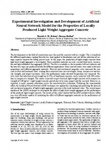
It could be seen in Figure 20 that there exists an error but the trend seems promising for extrapolation and prediction. To illustrate that accurate new weight vectors could be calculated, the ―Train Network ― button is pressed with the data from Case 4.The graph in Figure 21 shows the calculated data after training has been done. It can clearly be seen from Figure 21 that the newly calculated weights form Case 4 replicates the actual data accurately.

31

Figure 3.14 : Case 4 data after training on the pressure/temperature data.

32

4 Critical evaluation In open literature there exists a number of neural network methods explained in detail capable of interpolating sets of data point, however only recently much attention have been given in order to obtain neural network methods that can sufficiently be used to extrapolate data sets, for the application in feed forward process control. There exists neural network architecture that an achieve this, but it is very complex and difficult to apply in practice. However, the increasing popularity to use neural network prediction techniques is due to the desirability of using neuron networks to solve complex nonlinear systems instead of other forms of modelling. The log-sigmoid function that was used during this study seems to be a viable neural network method to solve trivial data sets, however when more complex data sets are used, the exponential method is lagging the completion. However, this being said, the exponential method is a very powerful tool; given enough data points, hidden layers and time it can complete any neural network prediction. The language packet used for this study was MS Excel®, which is a very powerful language pack for trivial mathematical applications. This was done due to many companies not having other language packets that are more appropriate for this study as mentioned later. A more appropriate language pack will be MATLAB®, Maple® or Mathematica® (Wolfram Mathematica, 2014) The use of an artificial neural network is to approximate the PV of the control processes, due to the difficulty of measuring the PV on-line. For example the concentration or fraction of a specific component in a liquid stream. By predicting the PV the system can accommodate any changes in the PV earlier than traditionally as a sample had to be taken for analysis and that could have meant that the plant was operating at a non-optimum point. The problem however with these neural networks are that the prediction is only for a certain interval and if this interval gets overshot the problem that occurs is much like that of sensor drifting the predicted PV is no longer valid. Thus the controller can no longer control the system. Some structures are specifically applicable to designated process units; therefore the neural network that was designed and used during this study is applicable to only a few different types of process units. If alterations in the process units are made and enough data points are given the neural network will take a long time to complete, resulting in possible delayed or inadequate results, therefore it will not be applied to a strong nonlinear process in which rapid alterations needs to be made. For such processes the tangent-sigmoid neural network 33

model will be more applicable. The exponential will be applied to processes with a large capacitance and most likely it will be connected to a PID controller in cascade. Due to the feed forward properties of neural networks, units such as exothermal reactors can be controlled more effectively compared to conventional generic model. It is harder to model the feed forward properties due to complicated equations, whereas the neural network, if trained properly, only gives a value of the feed forward portion. Resulting in more efficient process control.

34

5 Bibliography Baratt, i R., Vacca, G. & Servido, A. 1995. Neural networks modelling: application. (In Am Inst Chem Eng Annual Nov meeting. Miami. ) Boslovic, J.D. & Narendra, K.S. 1995. Comparison of linear, nonlinear and neural-networkbased

adaptive

controllers

for

a

class

of

fed-batch

fermentation

process. Automatica, 31(6):817-840. Chovan, T., Catfolis, T. & Meert, K. 1996. Neural network architecture for process control based on the RTRL algorithm. Chemical Engineering Journal, 42(2):493-502. Dorofki, M, Elshafie, AH, Jaafar, O, Karim, OJ & Mastura, S. 2012. Comparison of Artificial Neural Network Transfer Functions Abilities to Simulate Extreme Runoff Data. International Conference on Environment, Energy and Biotechnology.

(In

Singapore: IACSIT

Press. p. 1-6.) Elman, J.L.

1991.

Distributed Representations, Simple Recurrent Networks, and

Grammatical Structure. Machine Learning, 7(1):195-225. Fritzke, B. 1995. A growing neural gas network learns topologies. Advances in Neural Information Processing Systems , 7(3) Gardner, M.W & Dorling, SR.

1997.

Artificial Neural Networks (The Multilayer

Perceptron)ða Review OF Applications In The Atmospheric Sciences.

Atmospheric

Enviroment, 97:1352-2310. 20 February. Gershenson, C. 2014. Artificial Neural Networks for Beginners. Hagan, M.T. & Demuth, H.B.

1999. Neural Networks control. (In American control

Conference. p. 1642-1656.) Hayati, M & Shirvany, Y. 2007. Artificial Neural Network Approach for Short Term Load Forecasting for Illam Region. International journal of electrical,computer, and systems engineering, 1:1307-5179. Hebb, D. 1949. The organization of Behavior. London: Chapman & Hall, Limited. 169 p. Hussain, M.A. 1999. Review of the applications of neural networks in chemical process control

—

simulation

and

online

implementation.

Artificial

Intelligence

in

Engineering, 13(1):55-68. January.

35

Hussain, Mohamed Azlan. 1999. Review of the applications of neural networks in chemical process control Ð simulation and online implementation.

Arti®cial Intelligence in

Engineering, 13:55-68. Jain, A.K., Mao, J. & Mohiuddin. 1996. Artificial Neural Networks: A Tutorial. Theme Feature:31-43. March. Jha, G.K. 2011. Artificial neural networks and is applications. I.A.R.I., pp.41-50. Karlik, B. 2009. Performance Analysis of Various Activation Functions in Generalized MLP Architectures of Neural Networks. International Journal of Artificial Intelligence And Expert Systems, 1(4):111-122. Langonet, P.

1993. Neural nets for process control. (In Conference on Precision

Procesing Technology. Netherlands. p. 631-640.) Loh, A.P., Looi, K.O. & Fong, K.F. 1995. Neural network modelling and control strategies for a pH process. Journal of Process Control, 5(6):355–362. December. Patterson, D. 1996. Atrificial Neural Networks. Singapore: Prentice Hall. p. Psichogios, D.M. & Ungar, L.H. 1991. Direct and indirect model based control using artificial neural networks. Ind Engng Chem Res, 30:2564-2573. Sheppard, C.P., Gant, C.R. & Ward, R.M. 1992. A neural network based furnace. (In Proc Am Control Conference. p. 500-504.) Thiria, S, Mejia, C & Badran, F. 1993. A neural network approuch for modelling non-linear transfer functions. Journal of Geophysical Research, 98:2282-22841. Van Can, H.J., Bracke, H.A. & Hans, G.J. 1995. Design a real time testing of a neural model predictive controller for a nonlinear system. Chemical Engineering, 50(15):24192430. Wolfram

Mathematica.

2014.

Worfram

Mathematica

Neural

Networks. http://www.wolfram.com/products/applications/neuralnetworks/ Date of access: 11 April 2014. Ydstie,

B.E.

1990.

Forecasting

and

control

using

adaptive

connectionist

networks. Computers & Chemical Engineering, 14(4-5):583-599. May.

36

A

Appendix 1

User Manuel of the neural network This specific program was designed to be as user friendly as possible. What this means is that the user really has to do as little as possible. The interface looks as follow

The user firstly has to import 119 data values to the input area, which is marked with a grey shade this means user variables must be imported here. Once the three inputs and the outputs of the given inputs are imported simply click on the ―train network‖ button to run the network. Once the network has completed the learning process the program will display the following message.

After this message the program will direct the user to the relevant graphs to view the accuracy of the neural network.

A-1

B

Appendix 2 Source Code

This is where the internal working of the program will be discussed so that the reader has a better understanding of what happens behind the click of a button. For a better understanding see the (Cemi414_Project_equations_Group_7) program which will have all the equation visible. The following images show all the equations used in the excel spread sheet roughly but to gain

a

better

understanding

of

the

equations

used

open

the

MS

Excel®

(Cemi414_Project_equations_Group_7) attached to understand the working as only the first two iterations will be shown in the appendix. The following figure represented is sequenced in order, but in the program the figures is horizontally placed.

B-2

With this the following VBA code was used to iterate the data and to determine the error of the network. Private Sub CommandButton1_Click() Sheet1.Range("L5") = 0 Sheet1.Range("M5") = 0 Sheet1.Range("N5") = 0 Sheet1.Range("O5") = 0 Sheet1.Range("P5") = 0 Sheet1.Range("Q5") = 0 Sheet1.Range("R5") = 0 Sheet1.Range("S5") = 0 LR = 1 Sheet1.Cells(2, 8) = LR For epoks = 1 To 1000 If epoks = 1 Then inMse = Sheet1.Cells(5, 26) End If

B-3

Mse = Sheet1.Cells(5, 26) Sheet1.Cells(1, 12) = epoks / 10

Err1 = Sheet1.Cells(7, 19) Err2 = Sheet1.Cells(123, 19) Sheet1.Range("L5") = Sheet1.Range("L123") Sheet1.Range("M5") = Sheet1.Range("M123") Sheet1.Range("N5") = Sheet1.Range("N123") Sheet1.Range("O5") = Sheet1.Range("O123") Sheet1.Range("P5") = Sheet1.Range("P123") Sheet1.Range("Q5") = Sheet1.Range("Q123") Sheet1.Range("R5") = Sheet1.Range("R123") Sheet1.Range("S5") = Sheet1.Range("S123")

If (epoks = 200) And (Mse > (0.5 * inMse)) Then LR = LR + 1 Sheet1.Cells(2, 8) = LR Sheet1.Range("L5") = 0 Sheet1.Range("M5") = 0 Sheet1.Range("N5") = 0

B-4

Sheet1.Range("O5") = 0 Sheet1.Range("P5") = 0 Sheet1.Range("Q5") = 0 Sheet1.Range("R5") = 0 Sheet1.Range("S5") = 0 epoks = 0 End If If (epoks = 300) And (Mse > (0.3 * inMse)) Then LR = LR + 1 Sheet1.Cells(2, 8) = LR Sheet1.Range("L5") = 0 Sheet1.Range("M5") = 0 Sheet1.Range("N5") = 0 Sheet1.Range("O5") = 0 Sheet1.Range("P5") = 0 Sheet1.Range("Q5") = 0 Sheet1.Range("R5") = 0 Sheet1.Range("S5") = 0 epoks = 0 End If If ((Mse < 0.2) And (epoks < 1000)) Then epoks = 999 B-5

End If Next a = MsgBox("Program has fininshed training", vbInformation, "Info") Chart1.Activate

End Sub

B-6