Feb 9, 2008 - depends on processing classical âpaper mapâ into digital shape â made in raster format. ..... [7] Sitek Z.: Fotogrametria ogólna i inÄynieryjna.
GEOMATICS AND ENVIRONMENTAL ENGINEERING • Volume 1 • Number 3 • 2007
PaweÙ Hanus*
Application of Transformation with Conditions within Process of Boundaries Determination** 1. Foreword Using any kind of maps, especially cadastral ones, for boundaries determination, it is mostly necessary to scan them at first, and then to perform their suitable transformation to demanded, coordinates reference system. Scanning opearation depends on processing classical “paper map” into digital shape – made in raster format. Yet, the raster itself does not iclude so much information. One can say, that it is only a specific “picture”, until it is not processed into demanded form. Such map, called later “raster” does not have any geometric features, suitable for right use, especially in those surveying processes, where boundary plays an important role. It also does not have point coordinates in any existing coordinates reference system. Moreover, it is also influenced by various, random errors. Here they are [3]: – – – –
errors resulting from field survey, errors resulting from details mapping, errors resulting from using map, errors resulting from scanning map process.
Except mentioned above errors, cadastral raster map also includes systematic errors, coming from map shrinkage, and its age. Describing transformation process, one should mention at first, that suitable chosen transformation method, and suitable chosen control points serving this transformation, makes it possible to minimize the influence of almost all errors mentioned earlier or even to reject them complete. The only one exception are survey errors and control points errors. The other errors, as it was proved in [5] and [6], are possible to remove through choice suitable control points for transformation (their location, and their mutual * **
Faculty of Mining Surveying and Environmental Engineering, AGH University of Science and Technology, Krakow The work has been made within scientific University program no 11.11.150.837
49
50
P. Hanus
arrangement), and through proper kind of transformation. One should also remark, that wrong performed transformation may cause, in turn, enlarging these errors. One can state, that both kind of transformation and choice of control points for transformation, are strongly correlated each other. If we use conformal, Helmert transformation, arrangement of control points is essentially less important than accuracy of their location. Choosing, in turn, aĜne transformation, which is not conformal one, much more important problem is, first of all, suitable control points arrangement. Yet, an important factor is also accuracy of their location. Thus, choosing kind of transformation, one must be always conscious, what features it has, and what changes it causes. Without having such knowledge, results of transformation process may not be relevant. Application of documentation for boundaries determination, always demands great surveyor’s experience. Badly made estimation process of accessible documents, may lead to false conclusion. Badly performed boundary delimitation may cause next errors. So, suitable interpretation of cadastral documents for boundary determination process (while delimitation and subdivision) is crucial for its later performing. Taking into consideration a great variety of cadastral documentation existing in Poland, such estimation is mostly complicated.
2. Obtaining of control points In case of real estate delimitation and subdivision, an essential problem is the most accurate fiĴing-in rasters, prepared from existing maps, into the field local framework, near the real estate being an object of mentioned processes [3]. That is of no importance here raster deformation for points situated far from this real estate. Nevertheless, it is important, that the real estate, and real estate surrounding it, should be possibly accurate fit-in to the field. Obtaining control points in this case is essentially possible by two methods. The first method, not tiresome although giving wrong results, is using survey records, coming from surveying-legal processes, done on real estate, not necessary close to the real estate, being an object of actual survey. As an advantage of this method, one can mention, data accessibility without performing field survey. Yet, to such data one may not have full confidence. It comes from the fact, that some surveyors neglect their job sometimes, and that there is lack of scientific methods providing proper procedures of using such data. The second way of obtaining control points, for fiĴing-in raster, used while delimitation or subdivision, is field survey. This method seems to be much more confident and giving beĴer results, than the previous one. While survey one should
Application of Transformation with Conditions…
51
especially measure these details, which show boundary line. Nevertheless, one should accept some rules, resulting from field experience. First of all, one should be conscious, that exactly visible boundary in the field, one can find very seldom. An additional diĜculty, using cadastral map, is that they were prepared a long time ago. So, there are some details, which should be of great importance of the surveyor, while field survey. Here they are: – “three boundary strips”, that is a place determined by crossing three boundary lines in one point; – old trees, which were planted in boundary lines very oĞen; – points of old fences; – corners of old buildings. It is worth mentioning, that such details were used in the interwar period and aĞer the second world war, in order to supervise cadastral documentation of the former Austrian cadastre, existing in the southern part of Poland and used for various aims [1, 2]. One should remark, that – in case of lack such details in the direct neighbourhood of being measured real estate – one should expand the range of survey.
3. Application of transformation with conditions In case of some maps, especially cadastral ones, one may oĞen find there such circumstances, when parcel has been changed considerably through years [3]. Such case takes place, when parcels are located near roads or rivers and streams, and also in the neighbourhood of forests and timberlands. Such case is showed on figure. 1. In such case, one can not use, as control points, these boundary points, which are located in the neighbourhood of stream. One may also state, that obtained from raster map point, being located on the map exactly on the boundary line, should also be (aĞer transformation) situated on line, measured in the field, determined by any two points, located on boundary line, properly identified in the field. It seems to be in such a case, to run transformation, in which except obtaining “ordinary” control points there will be assumed also additional conditions, forcing locations of given point of cadastral map (primary reference coordinate system) on the line determined by two points obtained from field survey (secondary reference coordinate system). Of course, such conditions may be more than one. Such conditions one may add to any kind of transformation. In the paper, results of such approach, for aĜne transformation, have been showed.
52
P. Hanus
According to [7], such transformation is described by formulas (1): Xw = aX p + bYp + c Yw = dX p + eYp + f
(1)
where: Xw, Yw – point coordinates in secondary coordinate reference system, Xp, Yp – point coordinates in primary coordinate reference system, a, b, c, d, e, f – transformation coeĜcients.
Fig. 1. An example of area with changed boundaries of parcels, located near stream
Determination of transformation coeĜcients made in traditional approach, will be connected with arrangement of set of equations (mostly with additional equations), and then with determination, by means of least square method, transformation coeĜcients together with their point estimation. Determination of condition equation is based upon line equation, crossing two points. Coordinates of these two points are determined in secondary coordinate reference system (field system). Equation of the line crossing through point A ( Xw A, Yw A) and point B ( Xw B , Yw B) is y − Yw A =
Yw B − Yw A Xw B − Xw A
( x − Xw A)
(2)
Application of Transformation with Conditions…
53
Converting the equation (2) we receive: y = αx + β
(3)
where: α=
Yw B − Yw A
(4)
Xw B − Xw A
β = Yw A −
Yw B − Yw A Xw B − Xw A
Xw A
(5)
Assume in turn, that point C, aĞer transformation will be located on line AB (Fig. 2).
Fig. 2. Illustration of condition for point C, belonged to boundary line AB
Coordinates of point C ( Yp C , X p C ) are determined in primary coordinate reference system (cadastral map) and coordinates of points A ( Xw A , Yw A ) and B ( Xw B , Yw B ) are determined in secondary coordinate reference system (field system). Thus, one can write: XwC = aX pC + bYpC + c YwC = dX pC + eYpC + f
(6)
Substituting (6) to formula (3) we receive a(αX pC ) + b(αYpC ) + cα − dX pC − eYpC − f = −β
(7)
This is the condition equation for point C. In this equation, unknowns are only parameters a, b, c, d, e and f. One can also determine the rest values. Together with “usual” equations, arranged for the several control points, such set can be treated as a parametric model and solved by traditional least square method. Such set, may be wriĴen in the shape (8) A.X=L where: A – matrix of normal equations, X – unknown vector, L – vector of free factors.
54
P. Hanus
Matrix A will have, in case of application equations with conditions, the following shape: ⎡ X p1 ⎢ 0 ⎢ ⎢ . ⎢ ⎢ . A=⎢ . ⎢ ⎢α i X pi ⎢ . ⎢ ⎢ . ⎢ . ⎣
Yp1 0
1 0
0 X p1
0 Yp1
α i Ypi
αi
− X pi
−Ypi
.
.
.
.
0⎤ ⎡ Xw 1 ⎤ ⎢Y ⎥ 1⎥ ⎢ w1 ⎥ ⎥ . ⎥ ⎢ . ⎥ ⎢ ⎥ ⎥ . ⎥ ⎢ . ⎥ . ⎥ L=⎢ . ⎥ ⎢ ⎥ ⎥ −1⎥ ⎢ −βi ⎥ ⎢ . ⎥ ⎥ ⎢ ⎥ ⎥ ⎢ . ⎥ ⎥ ⎢ . ⎥ ⎥ ⎣ ⎦ ⎦
– equations created for “usual” control points,
– equation of condition for point i.
The values of transformation coeĜcients – vector X – using additionally weight matrix – P for several equations, we obtain from formula (9) X = (ATPA)-1 . ATPL One must pay aĴention, that in such approach, one must initialise some modification while calculation deviations computed on the base of obtained parameters of transformation of points coordinates. In case of points with condition, the best method is estimate the value of deviation on the base of distance of this point, aĞer transformation, from assumed line. If the distance diminished, and initialising additional equations did not increase the value of estimator of rest value Η, one can state, that fiĴing-in was correct. In order to check results of such approach, on the base of cadastral map, computations and analysis concerning some modelled examples, have been made. In the example number 1, shown on the figure 3, besides “usual” control points, the condition for point 5, has been added. This point, should be aĞer transformation, located on the line determined by points 16 and 17, which coordinates are known in the secondary coordinate reference system. Results of transformation with condition for point 5 shows figure 3. Errors of control points 1, 2, 3, and 4, and the distance of point 5 from the line 16–17, in case of traditional transformation and transformation with condition, shows table 1. It is visible, that deviations on control points did not change significantly while application additional condition. It is also visible, that point 5 is beĴer fit-on in the line 16–17. In the next example (number 2), shown on figure 4, we have two conditions. Point 6 should be situated, aĞer transformation, on the line 16–17, and point 8 should be located, aĞer transformation, on the line 18–19.
Application of Transformation with Conditions…
55
Fig. 3. Transformation with conditions – example 1
Table 1. Results of transformation – example 1
Point number
Deviations coordinates of control points of aĜne transformation with condition [m]
in traditional approach [m]
X1
–0.728
0.253
Y1
0.947
0.757
X2
–0.706
–0.263
Y2
–0.706
–0.791
X3
–0.135
0.251
Y3
0.828
0.753
X4
–1.190
–0.240
Y4
–0.536
–0.719
Distance of point 5 from line 16–17
0.101
0.916
Η
1.306
1.127
56
P. Hanus
Fig. 4. Transformation with conditions – example 2
One should remark, that it is also possible the case, when the only one condition is true, or the case, when two conditions are true. So, this case has been solved in three variants. At first, both conditions have been taken with the same weights. The second variant in turn, assumes bigger weight for point 8, confirming thus as probable wrong determination condition for point 6. The third variant, assumes bigger weight to condition for point 6, and less weight for condition for point 8. The list of results of transformation with conditions, in comparison with “usual” aĜne transformation, shows table 2.
Application of Transformation with Conditions…
57
Table 2. Results of transformation with conditions – example 2 AĜne transformation error in classical approach [m]
with conditions; bigger weight for point 8 [m]
with conditions; bigger weight for point 6 [m]
with conditions; equal weights for points 6 i 8 [m]
X1
0.156
–0.083
0.125
0.114
Y1
–0.524
0.398
–0.773
–0.520
X2
–0.064
–0.246
0.003
–0.057
Y2
0.182
0.468
–0.912
–0.252
X3
–0.093
–0.363
–0.187
–0.166
Y3
0.349
1.666
0.662
0.641
X4
0.002
0.232
0.148
0.092
Y4
0.011
–1.410
–0.913
–0.556
X5
–0.000
0.022
–0.162
–0.067
Y5
–0.018
0.652
1.654
0.780
Distance of point 6 from boundary measured in the field
2.984
3.464
0.032
1.776
Distance of point 8 from boundary measured in the field
1.369
0.052
2.876
1.857
Η
0.342
1.746
1.536
1.189
Number of point
On the base of table 2 results, it is visible that one condition is wrong. The most correct, from the point of view beĴer results, is the third variant, where bigger weight has been taken for point 6. In this case we have comparable deviations on “usual” control points, compared with traditional approach. Yet it is clear visible significant improvement of fiĴing-in point 6 on the line 16–17. The following example has been made on the base of data, collected while making expertise court maĴer [4]. In this case, 10 control points have been used with 4 conditions. The situation is showed on figure 5. Green points, showed on figure 5 are “usual” control points, while red points are those with conditions. Results obtained in this case have been showed in table 3.
58
P. Hanus
Fig. 5. Transformation with conditions – Zarzecze cadastral unit
Table 3. Results of transformation – example 3 Deviations coordinates of control points of aĜne transformation Number of point in traditional approach [m]
with conditions [m]
X1
0.125
0.156
Y1
0.059
0.313
X2
–0.122
–0.136
Y2
0.091
0.300
X3
–0.391
–0.311
Y3
–0.344
–0.160
X4
0.075
0.149
Y4
0.026
0.204
X5
0.331
0.390
Y5
0.087
0.249
X6
0.125
–0.070
Application of Transformation with Conditions…
59
Table 3 cd. Y6
0.059
–0.457
X7
–0.122
–0.065
Y7
0.562
0.602
condition 1
0.498
0.774
condition 2
0.554
0.296
condition 3
0.614
0.468
condition 4
0.321
0.158
Η
0.351
0.371
Obtained results, like in the previous examples, prove the idea of application such a method of transformation with conditions. The values of distances of points, from boundary line, have been significantly diminished as compared to traditional method. One should also mention, that presented problem can also be solved by means of using parametric model with additional conditions for unknowns it sems, that, obtained results should be similar.
4. Conclusion Given in the paper examples prove the possibility of using condition equations for computing transformation coeĜcients. It is especially useful in case of small quantity of control points or doubtful accuracy of these points. Adding to transformation equals conditions for chosen points, gives beĴer results than in case of ”usual” transformation. Moreover, this method can be used in case of lack of control points. Obtained results seem to be more correct than these, obtained by traditional methods. One should emphasize again, that results, obtained by this method, give satisfactory errors of boundary points location, of the real estate being the object of surveying-legal processes concerning delimitation and subdivision surveys.
References [1] Fedorowski W.: Ewidencja gruntów. PPWK, Warszawa 1974. [2] Frelek M., Fedorowski W., Nowosielski E.: Geodezja rolna. PPWK, Warszawa 1970.
60
P. Hanus
[3] Hanus P.: Ocena przydatnoïci dokumentacji byÙego katastru austriackiego dla potrzeb prac geodezyjnych. AGH, Kraków 2006 (rozprawa doktorska, niepublikowana). [4] Hanus P., Szczutko T.: Opinia wykonana na potrzeby Sdu Rejonowego w
ywcu w sprawie o rozgraniczenie nieruchomoïci – obr¿b Zarzecze. Kraków –
ywiec 2005. [5] Latoï S., Maïlanka J.: Cyfrowa mapa ewidencji gruntów i budynków w procesie budowania numerycznej bazy systemów informacji o terenie. MateriaÙy VIII Konferencji Naukowo-Technicznej, SIP, Warszawa 1998. [6] Maïlanka J.: Problemy prawne i techniczne synchronizacji danych geometrycznych i opisowych ewidencji gruntów. MateriaÙy Konferencji Naukowo-Technicznej, Piwniczna 2001. [7] Sitek Z.: Fotogrametria ogólna i inČynieryjna. PaÚstwowe Przedsi¿biorstwo Wydawnictw Kartograficznych im. Eugeniusza Homera, Warszawa – WrocÙaw 1991.