Applications of Computer Simulations and Statistical Mechanics in

Applications of Computer Simulations and Statistical Mechanics in Surface Electrochemistry P.A. Rikvold1,2 ,∗ I. Abou Hamad3 ,† T. Juwono1,‡ D.T. Robb4 ,§ and M.A. Novotny3,5¶

arXiv:0910.2185v1 [physics.chem-ph] 12 Oct 2009

1

Center for Materials Research and Technology, School of Computational Science, and Department of Physics, Florida State University, Tallahassee, FL 32306-4350, USA 2 National High Magnetic Field Laboratory, Tallahassee, FL 32310-3706, USA 3 HPC2 , Center for Computational Sciences, Mississippi State University, Mississippi State, MS 39762-5167, USA 4 Department of Physics, Clarkson University, Potsdam, NY 13699, USA 5 Department of Physics & Astronomy, Mississippi State University, Mississippi State, MS 39762-5167, USA

We present a brief survey of methods that utilize computer simulations and quantum and statistical mechanics in the analysis of electrochemical systems. The methods, Molecular Dynamics and Monte Carlo simulations and quantum-mechanical density-functional theory, are illustrated with examples from simulations of lithium-battery charging and electrochemical adsorption of bromine on single-crystal silver electrodes.

I.

INTRODUCTION

The interface between a solid electrode and a liquid electrolyte is a complicated many-particle system, in which the electrode ions and electrons interact with solute ions and solvent ions or molecules through several channels of interaction, including forces due to quantum-mechanical exchange, electrostatics, hydrodynamics, and elastic deformation of the substrate. Over the last few decades, surface electrochemistry has been revolutionized by new techniques that enable atomic-scale observation and manipulation of solid-liquid interfaces [1, 2], yielding novel methods for materials analysis, synthesis, and modification. This development has been paralleled by equally revolutionary developments in computer hardware and algorithms that by now enable simulations with millions of individual particles [3], so that there is now significant overlap between system sizes that can be treated computationally and experimentally. In this chapter, we discuss some of the methods available to study the structure and dynamics of electrodeelectrolyte interfaces using computers and techniques based on quantum and statistical mechanics. These methods are illustrated by some recent applications. The rest of the chapter is organized as follows. In Sec. II, we present fully three-dimensional, continuum simulations by Molecular Dynamics (MD) of ion intercalation during charging of Lithium-ion batteries. In Sec. III, we discuss the simplifications that are possible by mapping a chemisorption problem onto an effective lattice-gas (LG) Hamiltonian , and in Sec. IV we demonstrate how input parameters for a statisticalmechanical LG model can be estimated from quantum-mechanical density-functional theory (DFT) calculations. Section V is devoted to a discussion of Monte Carlo (MC) simulations, both for equilibrium problems (Sec. V A) and for dynamics (Sec. V B). As an example of the latter, we present in Sec. VI a simulational demonstration of a method to classify surface phase transitions in adsorbate systems, which is an extension of standard cyclic voltammetry (CV): the Electrochemical First-order Reversal Curve (EC-FORC) method. A concluding summary is given in Sec. VII.

∗ Electronic

address: address: ‡ Electronic address: § Electronic address: ¶ Electronic address: † Electronic

[email protected] [email protected] [email protected] [email protected] [email protected]

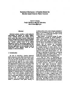
+ FIG. 1: (a) Snapshot of the model system containing four graphite sheets, two PF− 6 ions and ten Li ions (spheres), solvated in 69 propylene carbonate and 87 ethylene carbonate molecules after reaching constant volume in the N P T ensemble. (b) Snapshot after 200 ns MD simulation. The ensemble is the N V T ensemble. The system has periodic boundary conditions and is simulated at one atm and 300 K. Top view, perpendicular to the plane of the graphite sheets.

II.

MOLECULAR DYNAMICS SIMULATIONS OF ION INTERCALATION IN LITHIUM BATTERIES

The charging process in Lithium-ion batteries is marked by the intercalation of Lithium ions into the graphite anode material. Here we present MD simulations of this process and suggest a new charging method that has the potential for shorter charging times, as well as the possibility of providing higher power densities. A.

Molecular Dynamics and Model System

Molecular Dynamics is based on solving the classical equations of motion for a system of N atoms interacting through forces derived from a potential-energy function [4, 5, 6, 7, 8]. From the potential energy EP , the force on the ith atom, Fi , is calculated. Thus, the equation of motion is Fi (t) = −

∂EP ∂vi ∂ 2 ri = mi = mi 2 ∂ri ∂t ∂t

(1)

where ri , vi , and mi are the position, velocity, and mass of the ith atom, respectively. Consequently, the quality of the simulations strongly depends on the ability of the classical force field to reasonably describe the atomistic behavior. The newly developed General Amber Force Field (GAFF) [9] was used to approximate the bonded interactions of all the simulation molecules, while the simulation package Spartan (Wave-function, Inc., Irvine, CA) was used at the Hartree-Fock/6-31g* level to obtain the necessary point charges for each of the atoms. To simulate a charging field, the charge on the carbon atoms of the graphite sheets was set to −0.0125 e per atom. The bonded (first three terms of Eq. (2)) and non-bonded (last term) interactions in the AMBER Force Field are represented by the following potential-energy function: " # X X Aij X X Vn B q q ij i j (2) EP = [1 + cos(nφ − γ)] + Kr (r − req )2 + Kθ (θ − θeq )2 + 12 − R6 + ǫR 2 Rij ij ij i 0 favors adsorption. Equation (3) is also easily generalized to multiple species [24, 25]. To connect the electrochemical potentials to the concentrations in bulk solution of species X, [X], and the electrode potential, E, one has (in the dilute-solution approximation) Z E µ ¯x (T, [X], E) = µ ¯0x + kB T ln([X]/[X]0 ) − e γx (E ′ )dE ′ , (4) E0

where kB is Boltzmann’s constant, T the temperature, e the elementary charge, and γx (E) the electrosorption valency [26, 27, 28, 29] of X. The importance of the integral over the potential-dependent electrosorption valency (rather than just the product eγx (E)E) analogous to the case of potential-independent γx ) was pointed out in Ref. [30]. The quantities superscripted “0” are reference values that include local binding energies. The interaction constants and electrosorption valencies are effective parameters influenced by several physical effects, including electronic structure [21, 22, 23], surface deformation, (screened) electrostatic interactions [31, 32, 33], and the fluid electrolyte [34, 35]. The density conjugate to µ ¯x is the coverage relative to the number N of adsorption sites, X ci . (5) ΘX = N −1 i

IV.

CALCULATION OF LATTICE-GAS PARAMETERS BY DENSITY FUNCTIONAL THEORY

There are many methods to estimate lattice-gas parameters. One of these is comparison of MC simulations (see Sec. V) of a LG model with experimental adsorption isotherms. For detailed descriptions of this method we refer to Refs. [30, 31, 36, 37, 38, 39]. Here we instead concentrate on the purely theoretical method based on quantummechanical DFT calculations [23]. DFT is the most widely used method to calculate ground-state properties of many-electron systems. It is based on the Hohenberg-Kohn theorem, which states that all properties of the many-particle ground state can be expressed 4

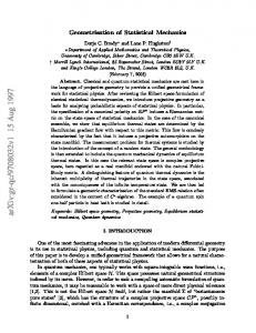
FIG. 3: (A) Cross section of a 3 × 3 supercell with Θ = 1/9. (B) Three-dimensional representation of the same cell and coverage. (C) Top view of a 3 × 3 surface and a 2 × 2 surface with various coverages.

in terms of the ground-state electron charge-density distribution [40] and leads to the Kohn-Sham equations for single-particle wave functions [41]. These are second-order differential equations, which include potential terms due to the ions and the classical Coulomb repulsive energy between the electrons, as well as the electronic exchangecorrelation energy, and they are solved self-consistently. For surface structural studies, DFT is usually performed using pseudopotentials with slab models and plane-wave basis sets. The slab consists of a finite number of atomic layers, periodic in the direction parallel to the surface, which can either be repeated periodically in the third direction (separated by a vacuum interval), or not. The fluid solvent can be considered either as an effective continuum, or by molecular models. Here we present preliminary results on a DFT calculation of lateral interaction constants pertaining to a latticegas model for the adsorption of Br on single-crystal Ag(100) surfaces [29, 37, 38, 39, 42]. The lattice-gas model is

5

˚, H3 = 0, infinitely repulsive interactions represented by Eq. (3) on a square lattice with lattice constant a = 2.95 A for adparticles at nearest-neighbor sites, and the long-range repulsion √ √ ( 2)3 (6) φnnn for rij ≥ 2 , φij = 3 rij which is compatible with dipole-dipole interactions or elastically mediated interactions. (Here, rij is given in units of a.) Since the DFT calculations are performed in the canonical ensemble (fixed adsorbate coverage), µ ¯ in Eq. (3) is replaced by the binding energy of a single adparticle, Eb . We prepared slabs with seven metal layers, which were placed inside a supercell with periodic boundary conditions. Two different sizes of supercells were used: a 2 × 2 supercell with the size of 2a × 2a × 36.95 ˚ A, and a 3 × 3 supercell with the size of 3a × 3a × 36.95 ˚ A. The vacuum region above the surface was twice the thickness of the slab, and the orientation of the surface normal was in the z direction. One, two, and three Br atoms were placed on the 3 × 3 surface to represent coverages Θ = 1/9, 2/9, and 1/3. Two Br atoms were placed on the 2 × 2 surface to represent Θ = 1/2, and one to represent Θ = 1/4. Supercells with different coverages of Br are shown in Fig. 3. The DFT calculations were performed using the Vienna Ab Initio Simulation Package (VASP) [43, 44, 45]. The basis set was plane-wave, with the generalized gradient-corrected exchange-correlation function [46, 47], and Vanderbilt pseudopotentials [48]. The k-point mesh was generated using the Monkhorst method [49] with a 5 × 5 × 1 grid for the 3 × 3 cells and a 7 × 7 × 1 grid for the 2 × 2 cells. All calculations were done on a 54 × 54 × 192 real-space grid. Individual DFT calculations provide total energies, E, and charge densities, ρ(~x). The adsorption energy Eads for a single adatom and the corresponding charge-transfer function ∆ρ(~x) are obtained from calculations of the adsorbed system and isolated slab and atoms as follows: Eads = [Esyst − Eslab ] /Nads − EBr

(7)

∆ρ(~x) = [ρ(~x)syst − ρ(~x)slab ]/Nads − ρ(~x)Br ,

(8)

and [50]

where Nads = N Θ is the number of adsorbed Br atoms in the cell, and the quantities subscripted Br refer to a single, isolated Br atom. Since the system is electrically neutral, the integral over space of ∆ρ(~x) vanishes. The surface dipole moment is defined as Z p = z∆ρ(z)dz . (9) Kohn and Lau [51] have shown that the non-oscillatory part of the dipole-dipole interaction energy between adsorbates separated by a distance R behaves as φdip−dip =

2pa pb 4πǫ0 R3

(10)

for large R (in our case larger than the nearest-neighbor distance). This result is twice what one might na¨ıvely expect. Thus, the next-nearest-neighbor interaction constant from Eq. (6) would be φdip−dip

nnn

=

2p2 3 4πǫ0 Rnnn

(11)

with p obtained from the DFT by Eq. (9). This estimate, which depends on Θ, is included in Fig. 4 as solid circles. Alternatively, the interaction constant φnnn in the LG Hamiltonian, Eq. (3), can be estimated by performing a nonlinear least-squares fit of the Θ-dependent DFT adsorption energy Eads in Eq. (7) to Eads = −φnnn ΣΘ − Eb Θ

(12)

with φnnn = A(1 + BΘ)2 , using the three fitting parameters A, B, and Eb . This is consistent with the theoretical prediction of Eq. (11) with a dipole moment that depends linearly on Θ. The quantity √ ( 2)3 X ci cj (13) ΣΘ = 3 N i