Applications of resampling methods in actuarial practice - CiteSeerX

job no. 1969

casualty actuarial society

CAS journal

1969D04 [1]

11-08-01

4:58 pm

APPLICATIONS OF RESAMPLING METHODS IN ACTUARIAL PRACTICE RICHARD A. DERRIG, KRZYSZTOF M. OSTASZEWSKI, AND GRZEGORZ A. REMPALA

Abstract Actuarial analysis can be viewed as the process of studying profitability and solvency of an insurance firm under a realistic and integrated model of key input random variables such as loss frequency and severity, expenses, reinsurance, interest and inflation rates, and asset defaults. Traditional models of input variables have generally fitted parameters for a predetermined family of probability distributions. In this paper we discuss applications of some modern methods of non-parametric statistics to modeling loss distributions, and possibilities of using them for modeling other input variables for the purpose of arriving at an integrated company model. Several examples of inference about the severity of loss, loss distributions percentiles and other related quantities based on data smoothing, bootstrap estimates of standard error and bootstrap confidence intervals are presented. The examples are based on reallife auto injury claim data and the accuracy of our methods is compared with that of standard techniques. Model adjustment for inflation and bootstrap techniques based on the Kaplan–Meier estimator, useful in the presence of policies limits (censored losses), are also considered. ACKNOWLEDGEMENT The last two authors graciously acknowledge support from the Actuarial Education and Research Fund.

322

job no. 1969


CAS journal

1969D04 [2]

11-08-01

4:58 pm

APPLICATIONS OF RESAMPLING METHODS IN ACTUARIAL PRACTICE

323

1. INTRODUCTION In modern analysis of the financial models of propertycasualty companies the input variables can be typically classified into financial variables and underwriting variables (e.g., see D’Arcy, Gorvett, Herbers and Hettinger [6]). The financial variables generally refer to asset-side generated cash flows of the business, and the underwriting variables relate to the cash flows of the liabilities side. The process of developing any actuarial model begins with the creation of probability distributions of these input variables, including the establishment of the proper range of values of input parameters. The use of parameters is generally determined by the use of parametric families of distributions. Fitting of those parameters is generally followed either by Monte Carlo simulation together with integration of all inputs for profit testing and optimization, or by the study of the effect of varying the parameters on output variables in sensitivity analysis and basic cash flow testing. Thus traditional actuarial methodologies are rooted in parametric approaches, which fit prescribed distributions of losses and other random phenomena studied (e.g., interest rate or other asset return variables) to the data. The experience of the last two decades has shown greater interdependence of basic loss variables (severity, frequency, exposures) with asset variables (interest rates, asset defaults, etc.), and sensitivity of the firm to all input variables. Increased complexity has been accompanied by increased competitive pressures, and more frequent insolvencies. In our opinion, in order to properly address these issues one must carefully address the weaknesses of traditional methodologies. These weaknesses can be summarized as originating from either ignoring the uncertainties of inputs, or mismanaging those uncertainties. While early problems of actuarial modeling could be attributed mostly to ignoring uncertainty, we believe at this point the uncertain nature of model inputs is generally acknowledged. Note that Derrig and Ostaszewski [9] used fuzzy set techniques to handle the mixture of probabilistic and non-probabilistic uncertainties in asset/

job no. 1969

324


CAS journal

1969D04 [3]

11-08-01

4:58 pm


liability considerations for property-casualty claims. In our opinion it is now time to proceed to deeper issues concerning the actual forms of uncertainty. The Central Limit Theorem and its stochastic process counterpart provide clear guidance for practical uses of the normal distribution and all distributions derived from it. But one cannot justify similarly fitting convenient distributions to, for instance, loss data and expect to easily survive the next significant change in the marketplace. What does work in practice, but not in theory, may be merely an illusion of applicability provided by powerful tools of modern technology. If one cannot provide a justification for the use of a parametric distribution, then a nonparametric alternative should be studied, at least for the purpose of understanding the firm’s exposures. In this work, we will show such a study of nonparametric methodologies applied to loss data, and will advocate the development of an integrated company model with the use of nonparametric approaches. 1.1. Loss Distributions We begin by addressing the most basic questions concerning loss distributions. The first two parameters generally fitted to the data are average claim size and the number of claim occurrences per unit of exposure. Can we improve upon these estimates by using nonparametric methods? Consider the problem of estimating the severity of a claim, which is, in its most general setting, equivalent to modeling the probability distribution of a single claim size. Traditionally, this has been done by means of fitting some parametric models from a particular continuous family of distributions (e.g., see Daykin, Pentikainen, and Pesonen [7, Chapter 3]). While this standard approach has several obvious advantages, we should also realize that occasionally it may suffer some serious drawbacks: ! Some loss data has a tendency to cluster about round numbers like $1,000, $10,000, etc., due to rounding off the claim

job no. 1969


CAS journal

1969D04 [4]

11-08-01

4:58 pm


325

amount and thus in practice follows a mixture of continuous and discrete distributions. Usually, parametric models simply ignore the discrete component in such cases. ! The data is often truncated from below or censored from above due to deductibles and/or limits on different policies. In particular, the presence of censoring, if not accounted for, may seriously compromise the goodness-of-fit of a fitted parametric distribution. On the other hand, trying to incorporate the censoring mechanism (which is often random in its nature, especially when we consider losses falling under several insurance policies with different limits) often leads to a creation of a very complex model which is difficult to work with. ! The loss data may come from a mixture of distributions depending upon some known or unknown classification of claim types. ! Finally, it may happen that the data simply does not fit any of the available distributions in a satisfactory way. It seems, therefore, that there are many situations of practical importance where the traditional approach cannot be utilized, and one must look beyond parametric models. In this work we point out an alternative, nonparametric approach to modeling losses and other random parameters of financial analysis, originating from the modern methodology of nonparametric statistics based on the bootstrap or resampling method. To keep things in focus we will be concerned here only with applications to modeling the severity of loss, but the methods discussed may be easily applied to other problems such as loss frequencies, asset returns, asset defaults, and the combination of variables into models of Risk Based Capital, Value at Risk, and general Dynamic Financial Analysis (DFA), including Cash Flow Testing and Asset Adequacy Analysis.

job no. 1969

326


CAS journal

1969D04 [5]

11-08-01

4:58 pm


1.2. The Concept of Bootstrap The concept of bootstrap was first introduced in the seminal piece of Efron [10], and relies on the consideration of the discrete empirical distribution generated by a random sample of size n from an unknown distribution F. This empirical distribution assigns equal probability to each sample item. In the dis! for that distribution. By cussion which follows, we will write F n generating an independent, identically distributed (IID) random ! or its appropriately sequence (resample) from the distribution F n smoothed version, we can arrive at new estimates of various parameters and nonparametric characteristics of the original distribution F. This idea is at the very root of the bootstrap methodology. In particular, Efron [10] points out that the bootstrap gives a reasonable estimate of standard error for any estimator, and it can be extended to statistical error assessments and to inferences beyond biases and standard errors. 1.3. Overview of the Article In this paper, we apply bootstrap methods to two data sets as illustrations of the advantages of resampling techniques, especially when dealing with empirical loss data. The basics of bootstrap theory are covered in Section 2, where we show its applications in estimating standard errors and calculating confidence intervals. In Section 3, we compare bootstrap and traditional estimators for quantiles and excess losses using some truncated wind loss data. The important concept of smoothing the bootstrap estimator is also covered in that section. Applications of bootstrap to auto bodily injury liability claims in Section 4 show loss elimination ratio estimates together with their standard errors in a case of lumpy and clustered data (the data set is enclosed in Appendix B). More complicated designs that incorporate data censoring and adjustment for inflation appear in Section 5. Sections 6 and 7 provide some final remarks and conclusions. The Mathematica 3.0 programs used to perform bootstrap calculations are provided in Appendix A.

job no. 1969


CAS journal

1969D04 [6]

11-08-01

4:58 pm


327

2. BOOTSTRAP STANDARD ERRORS AND CONFIDENCE INTERVALS

As we have already mentioned in the previous section, the central idea of bootstrap lies in sampling the empirical cumula! . This idea is closely related tive distribution function (CDF) F n to the following, well-known statistical principle, henceforth referred to as the “plug-in” principle. Given a parameter of interest µ(F) depending upon an unknown population CDF F, we esti! ). That is, we simply replace F in mate this parameter by µˆ = µ(F n ! obtained from the formula for µ by its empirical counterpart F n the observed data. The plug-in principle will not provide good ! poorly approximates F, or if there is information results if F n about F other than that provided by the sample. For instance, in some cases we might know (or be willing to assume) that F belongs to some parametric family of distributions. However, the plug-in principle and the bootstrap may be adapted to this latter situation as well. To illustrate the idea, let us consider a parametric family of CDF’s "F¹# indexed by a parameter ¹ (possibly a ! 0 denote its estimate calcuvector), and for some given ¹0 , let ¹ lated from the sample. The plug-in principle in this case states that we should estimate µ(F¹0 ) by µ(F¹!0 ). In this case, bootstrap is often called parametric, since a resample is now collected from F¹!0 . Here and elsewhere in this work, we refer to any replica of µˆ calculated from a resample as “a bootstrap estimate of µ(F)” and denote it by µˆ $ . 2.1. The Bootstrap Methodology Bickel and Freedman [2] formulated conditions for consistency of bootstrap, which resulted in further extensions of Efron’s [10] methodology to a broad range of standard applications, including quantile processes, multiple regression and stratified sampling. They also argued that the use of bootstrap did not require theoretical derivations such as function derivatives, influence functions, asymptotic variances, the Edgeworth expansion, etc.

job no. 1969

328


CAS journal

1969D04 [7]

11-08-01

4:58 pm


Singh [19] made a further point that the bootstrap estimator of the sampling distribution of a given statistic may be more accurate than the traditional normal approximation. In fact, it turns out that for many commonly used statistics the bootstrap is asymptotically equivalent to the one-term Edgeworth expansion estimator, usually having the same convergence rate, which is faster than the normal approximation. In many more recent statistical texts the bootstrap is recommended for estimating sampling distributions and finding standard errors and confidence sets. The extension of the bootstrap method to the case of dependent data was considered for instance by Ku¨ nsch [15], who suggested a moving block bootstrap procedure which takes into account the dependence structure of the data by resampling blocks of adjacent observations rather than individual data points. More recently, Politis and Romano [16] suggested a method based on circular blocks (i.e., on wrapping the observed time series values around the circle and then generating the blocks of the bootstrap data from the circle’s “arcs”). In the case of the sample mean this method, which is known as circular bootstrap, again was shown to accomplish the Edgeworth correction for dependent, stationary data. The bootstrap methods can be applied to both parametric and non-parametric models, although most of the published research in the area is concerned with the non-parametric case since that is where the most immediate practical gains might be expected. Let us note though that a simple, non-parametric bootstrap may often be improved by other bootstrap methods taking into account the special nature of the model. In the IID non-parametric models, for instance, the smoothed bootstrap (bootstrap based on ! ) often improves the simple bootsome smoothed version of F n ! ). Since in recent years sevstrap (bootstrap based solely on F n eral excellent books on the subject of resampling and related techniques have become available, we will not be particularly concerned here with providing all the details of the presented techniques, contenting ourselves with making appropriate ref-

job no. 1969


CAS journal

1969D04 [8]

11-08-01

4:58 pm


329

erences to more technically detailed works. Readers interested in gaining some basic background in resampling are referred to Efron and Tibisharani [11]. For a more mathematically advanced treatment of the subject, we recommend Shao and Tu [17]. 2.2. Bootstrap Standard Error Estimate Arguably, one of the most important applications of bootstrap ˆ It is to provide an estimate of the standard error of µˆ (seF (µ)). is rarely practical to calculate it exactly; instead, one usually ˆ with the help of multiple resamples. The approximates seF (µ) approximation to the bootstrap estimate of standard error of µˆ (or BESE) suggested by Efron [10] is given by !B = se

" B #

b=1

[µˆ $ (b) % µˆ $ (&)]2 =(B % 1)

$1=2

,

(2.1)

%

where µ $ (&) = Bb=1 µˆ $ (b)=B, B is the total number of resamples (each of size n) collected with replacement from the plug-in estimate of F (in the parametric or non-parametric setting), and µˆ $ (b) is the original statistic µˆ calculated from the bth resample (b = 1, : : : , B). By the law of large numbers ˆ ! B = BESE(µ), lim se

B'(

and, for sufficiently large n, we expect ˆ ) se (µ): ˆ BESE(µ) F Let us note that B, the total number of resamples, may be as large as we wish since we are in complete control of the resampling process. It has been shown that for estimating the standard error, one should take B to be about 250, whereas for different resampled statistics this number may have to be significantly increased in order to reach the desired accuracy (see [11]).

job no. 1969

330


CAS journal

1969D04 [9]

11-08-01

4:58 pm


2.3. The Method of Percentiles Let us now turn to the problem of using the bootstrap methodology to construct confidence intervals. This area has been a major focus of theoretical work on the bootstrap, and several different methods of approaching the problem have been suggested. The “naive” procedure described below is not the most efficient one and can be significantly improved in both rate of convergence and accuracy. It is, however, intuitively obvious and easy to justify, and seems to be working well enough for the cases considered here. For a complete review of available approaches to bootstrap confidence intervals, see [11]. Let us consider µˆ $ , a bootstrap estimate of µ based on a resample of size n from the original sample X1 , : : : , Xn , and let G$ be its distribution function given the observed sample values G$ (x) = P"µˆ $ * x + X1 = x1 , : : : , Xn = xn #: Recall that for any distribution function F and p , (0, 1) we define the pth quantile of F (sometimes also called pth percentile) as F %1 (p) = inf"x : F(x) - p#. The bootstrap percentiles method gives G$%1 (®) and G$%1 (1 % ®) as, respectively, lower and upper ˆ Let us note that bounds for the (1 % 2®) confidence interval for µ. ˆ for most statistics µ, the distribution function of the bootstrap estimator µˆ $ is not available. In practice, G$%1 (®) and G$%1 (1 % ®) are approximated by taking multiple resamples and then calculating the empirical percentiles. In this case the number of resamples B is usually much larger than for estimating BESE; in most cases B - 1000 is recommended. 3. BOOTSTRAP AND SMOOTHED BOOTSTRAP ESTIMATORS VS TRADITIONAL METHODS

In making the case for the usefulness of bootstrap methodology in modeling loss distributions, we would first like to compare its performance with that of the standard methods of inference as presented in actuarial textbooks.

job no. 1969


CAS journal

1969D04 [10]

11-08-01

4:58 pm


331

3.1. Application to Wind Losses: Quantiles Let us consider the following set of 40 losses due to windrelated catastrophes that occurred in 1977. These data are taken from Hogg and Klugman [12], where they are discussed in detail in Chapter 3. The losses were recorded only to the nearest $1,000,000 and data included only those losses of $2,000,000 or more. For convenience they have been ordered and recorded below. 2, 2, 2, 2, 2, 2, 2, 2, 2, 2 2, 2, 3, 3, 3, 3, 4, 4, 4, 5 5, 5, 5, 6, 6, 6, 6, 8, 8, 9 15, 17, 22, 23, 24, 24, 25, 27, 32, 43 Using this data set we shall give two examples illustrating the advantages of applying the bootstrap approach to modeling losses. The problem at hand is a typical one: assuming that all the losses recorded above have come from a single unknown distribution F, we would like to use the data to obtain some good approximation for F and its various parameters. First, let us look at an important problem of finding the approximate confidence intervals for the quantiles of F. The standard approach to this problem relies on the normal approximation to the sample quantiles (order statistics). Applying this method, Hogg and Klugman [12] have found the approximate 95% confidence interval for the 0.85th quantile of F to be between X30 and X39 , which for the wind data translates into the observed interval (9, 32). They also have noted that “this is a wide interval but without additional assumptions this is the best we can do.” Is that really true? To answer this question let us first note that in this particular case the highly skewed binomial distribution of the 0.85th sample quantile is approximated by a symmetric normal curve. Thus, it seems reasonable to expect that normal approximation could be improved here upon introducing some form of correction for skewness. In the standard normal

job no. 1969

332


CAS journal

1969D04 [11]

11-08-01

4:58 pm


approximation theory this is usually accomplished by considering, in addition to the normal term, the first non-normal term in the asymptotic Edgeworth expansion of the binomial distribution. The resulting formula is messy and requires the calculation of a sample skewness coefficient, as well as some refined form of the continuity correction (e.g., see Singh [19]). On the other hand, the bootstrap has been known to make such a correction automatically (Singh [19]) and hence we could expect that a bootstrap approximation would perform better here.1 Indeed, in this case (in the notation of Section 2) we have µ(F) = F %1 (0:85) and ! %1 (0:85) ) X , the 34th order statistic, which for the wind µˆ = F (34) n data equals 23. For sample quantiles the bootstrap distribution G$ can be calculated exactly (Shao and Tu [17, p.10]) or approximated by an empirical distribution obtained from B resamples as described in Section 2. Using either method, the (1 % 2®) confidence interval calculated using the percentile method is found to be between X(28) and X(38) (which is also in this case the exact confidence interval obtained by using binomial tables). For the wind data this translates into the interval (8, 27), which is considerably shorter than the one obtained by Hogg and Klugman [12]. 3.2. The Smoothed Bootstrap and its Application to Excess Wind Losses As our second example, let us consider the estimation of the probability that a wind loss will exceed a $29,500,000 threshold. In our notation that means that we wish to estimate the unknown parameter (1 % F(29:5)). A direct application of the plug-in principle gives the value 0.05, the nonparametric estimate based on relative frequencies. However, note that the same number is also an estimate for (1 % F(29)) and (1 % F(31:5)), since the relative 1 This turns out to be true only for a moderate sample size (here, 40); for a binomial distribution with large n (i.e., large sample size) the effect of the bootstrap correction is negligible. In general, the bootstrap approximation performs better than the normal approximation for large sample sizes only for continuous distributions.

job no. 1969


CAS journal

1969D04 [12]

11-08-01

4:58 pm


333

frequency changes only at the threshold values present in reported data. In particular, since the wind data were rounded off to the nearest unit, the nonparametric method does not give a good estimate for any non-integer threshold. This problem with the same threshold value of $29,000,000 was also considered in [12, Example 4 on p. 94 and Example 1 on p. 116]. As indicated therein, one reasonable way to deal with the non-integer threshold difficulty is to first fit some continuous curve to the data. The idea seems justified since the clustering effect in the wind data has most likely occurred due to rounding off the records. In their book Hogg and Klugman [12] have used standard techniques based on method of moments and maximum likelihood estimation to fit two different parametric models to the wind data: the truncated exponential with CDF F¹ (x) = 1 % e%(x%1:5)=¹ ,

1:5 < x < (

(3.1)

for ¹ > 0, and the truncated Pareto with CDF F®,¸ (x) = 1 %

&

¸ ¸ + x % 1:5

'®

,

1:5 < x < (

(3.2)

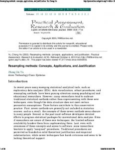
for ® > 0, ¸ > 0. For the exponential distribution the method of moments estimator as well as maximum likelihood estimator (MLE) of ¹ was found to be ¹ˆ = 7:725. The MLE’s for the Pareto distribution parameters were ¸ˆ = 28:998 and ®ˆ = 5:084; similar values were obtained using the method of moments. The empirical distribution function for the wind data along with two fitted maximum likelihood models are presented in Figure 1. The solid smooth line represents the curve fitted from the exponential family (3.1), the dashed line represents the curve fitted from the Pareto family (3.2), and a vertical line is drawn for reference at x = 29:5. It is clear that the fit is not good at all, especially around the interval (16, 24). The reason for the bad fit is the fact that both fitted curves are consistently concave down

job no. 1969

334


CAS journal

1969D04 [13]

11-08-01

4:58 pm


FIGURE 1 EMPIRICAL AND FITTED CDF’S FOR WIND LOSS DATA

for all the x’s and F seems to be concave up in this area.2 The fit in the tail seems to be much better. Once we determine the values of the unknown model parameters, MLE estimators for (1 % F(29:5)) may be obtained from (3.1) and (3.2). The numerical values of these estimates, their respective variances and their 95% confidence intervals are summarized in the second and third row of Table 1. All the confidence intervals and variances for the first three estimates shown in the table are calculated using the normal theory approximation. The variance and confidence intervals for the fourth estimate based on the moving-average smoother are calculated by 2 In practice, this drawback could be possibly remedied by fitting a mixture of the distributions shown in (3.1) and (3.2). However, this approach could considerably complicate the parametric model and seems unlikely to provide much improvement in the tail fit, which is of primary interest here.

job no. 1969


CAS journal

1969D04 [14]

11-08-01

4:58 pm


335

TABLE 1 COMPARISON OF THE PERFORMANCE OF ESTIMATORS FOR (1 % F(29:5)) FOR THE WIND DATA Fitted Model Non-parametric (Plug-in) Exponential Pareto 3-Step Moving Average Smoother

Estimate of (1 % F(29:5))

Approx. s.e.

Approx. 95% c.i. (two sided)

0.05 0.027 0.036

0.034 0.015 0.024

(%0:019, 0:119) (%0:003, 0:057) (%0:012, 0:084)

0.045

0.016

(0:013, 0:079)

means of the approximate BESE and bootstrap percentile methods described in Section 2. In the first row the same characteristics are calculated for the standard non-parametric estimate based on relative frequencies. As we may well see, the respective values of the point estimators differ considerably from model to model and, in particular, both MLE’s are quite far away from the relative frequency estimator. Another thing worth noticing is that the confidence intervals for all three models have negative lower bounds—they are obviously too long, at least on one side. This also indicates that their true coverage probability may in fact be greater than 95%. In order to provide a better estimate of (1 % F(29:5)) for the wind data, we will first need to construct a smoothed version of the empirical CDF. In order to do so we employ the following data transformation widely used in image and signal processing theory, where a series of raw data "x1 , x2 , : : : , xn # is often transformed to a new series of data before it is analyzed. The purpose of this transformation is to smooth out local fluctuations in the raw data, so the transformation is called data smoothing or a smoother. One common type of smoother employs a linear transformation and is called a linear filter. A linear filter with weights "c , c , : : : , cr%1 # transforms the given data to weighted averages %0r%11 j=0 cj xt%j for t = r, r + 1, : : : , n. Notice that the new data set has

job no. 1969

336


CAS journal

1969D04 [15]

11-08-01

4:58 pm


FIGURE 2 EMPIRICAL AND SMOOTHED CDF’S FOR WIND LOSS DATA

length (n % r % 1). If all the weights ck are equal and they sum to unity, the linear filter is called an r-term moving average. For an overview of this interesting technique and its various applications, see Simonoff [18]. To create a smoothed version of the empirical CDF for the wind data, we have first used a three-term moving average smoother and then linearized in between any two consecutive data points. The plot of this linearized smoother along with the original empirical CDF is presented in Figure 2. A vertical line is once again drawn for reference at x = 29:5. Let us note that the smoother follows the “concave-up-down-up” pattern of the data, which was not the case with the parametric distributions fitted from the families (3.1) and (3.2). Once we have constructed the smoothed empirical CDF for the wind data, we may simply read the approximate value of

job no. 1969


CAS journal

1969D04 [16]

11-08-01

4:58 pm


337

(1 % F(29:5)) off the graph (or better yet, ask the computer to do it for us). The resulting numerical value is 0.045. What is the standard error for that estimate? We again may use the bootstrap to answer that question without messy calculations. An approximate value for BESE (with B = 1000, but the result is virtually the same for B = 100) is found to be 0.016, which is only slightly worse than that of the exponential model MLE and much better than the standard error for the Pareto and empirical models. Equivalently, the same result may be obtained by numerical integration. Finally, the 95% confidence interval for (1 % F(29:5)) is found by means of the bootstrap percentile method with the number of replications set at B = 1000. Here the superiority of the bootstrap is obvious, as it gives an interval which is the second shortest (again exponential MLE model gives a shorter interval) but, most importantly, is bounded away from zero. The results are summarized in Table 1. Let us note that the result based on a smoothed empirical CDF and bootstrap dramatically improves that based on the relative frequency (plug-in) estimator and standard normal theory. It is perhaps of interest to note also that the MLE estimator of (1 % F(29:5)) in the exponential model is simply a parametric bootstrap estimator. For more details on the connection between MLE estimators and bootstrap, see [11]. 4. CLUSTERED DATA In the previous section we have assumed that the wind data were distributed according to some continuous CDF F. Clearly this is not always the case with loss data, and in general we may expect our theoretical loss distribution to follow some mixture of discrete and continuous CDF’s. 4.1. Massachusetts Auto Bodily Injury Liability Data In Appendix B we present the set of 432 closed losses due to bodily injuries in car accidents, under bodily injury liability (BI) policies reported in the Boston Territory (19) for calendar year

job no. 1969

338


CAS journal

1969D04 [17]

11-08-01

4:58 pm


1995 (as of mid-1997). The losses are recorded in thousands and are subject to various policy limits but have no deductible. Policy limits capped 16 out of 432 losses which are therefore considered right-censored. The problem of bootstrapping censored data will be discussed in the next section; here we would like to concentrate on another interesting feature of the data. Massachusetts BI claim data are of interest because the underlying behavioral processes have been analyzed extensively. Weisberg and Derrig [20] and Derrig, Weisberg and Chen [8] describe the Massachusetts claiming environment after a tort reform as a “lottery” with general damages for non-economic loss (pain and suffering) as the prize. Cummins and Tennyson [5] showed signs of similar patterns countrywide, while Carroll, Abrahamse and Vaiana [3] and the Insurance Research Council [13] documented the pervasiveness of the lottery claims in both tort and no-fault state injury claim payment systems. The overwhelming presence of suspected fraud and buildup claims3 allow for distorted relationships between the underlying economic loss and the liability settlement. Claim negotiators can greatly reduce the “usual” non-economic damages when exaggerated injury and/or excessive treatment are claimed as legitimate losses. Claim payments in such a negotiated process with discretionary injuries tend to be clustered at some usual mutually-acceptable amounts, especially for the run-of-the-mill strain and sprain claims. Conners and Feldblum [4] suggest that the claim environment, rather than the usual rating variables, are the key elements needed to understand and estimate relationships in injury claim data. All the data characteristics above tend to favor empirical methods over analytical ones. Looking at the frequencies of occurrences of the particular values of losses in Massachusetts BI claim data, we may see that several numerical values have especially high frequency. The loss 3 In auto insurance, fraudulent claims are those in which there was no injury or the injury was unrelated to the accident, whereas buildup claims are those in which the injury is exaggerated and/or the treatment is excessive.

job no. 1969


CAS journal

1969D04 [18]

11-08-01

4:58 pm


339

FIGURE 3 APPROXIMATION TO THE EMPIRICAL CDF FOR THE BI DATA ADJUSTED FOR THE CLUSTERING EFFECT

of $5,000 was reported 21 times (nearly 5% of all the occurrences), the loss of $20,000 was reported 15 times, $6,500 and $4,000 losses were reported 14 times, a $3,500 loss was only slightly less common (13 times), and losses of size $6,000 and $9,000 occurred 10 times each. There were also several other numerical values that have occurred at least five times. The clustering effect is obvious here and it seems that we should incorporate it into our model. This may be accomplished for instance by constructing an approximation to the empirical CDF, which is linearized in between the observed data values except for the ones with high frequency, where it behaves like the original, discrete CDF. In Figure 3 we present such an approximate CDF for the BI data. We have allowed our adjusted CDF to have discontinuities at the observed values which occurred with frequencies of five or greater. The left panel of Figure 3 shows the graph plotted for the entire range of observed loss values (0, 25). The right panel zooms in on the values from 3.5 to 5.5. Discontinuities can be seen here as the graph’s “jumps” at the observed loss values of high frequency: 3.5, 4, 4.5, 5. 4.2. Bootstrap Estimates for Loss Elimination Ratios To give an example of statistical inference under this model, let us consider a problem of eliminating part of the BI losses

job no. 1969

340


CAS journal

1969D04 [19]

11-08-01

4:58 pm


by purchasing a reinsurance policy that would cap the losses at some level d. Since the BI data is censored at $20,000, we would consider here only values of d not exceeding $20,000. One of the most important problems for the insurance company considering purchasing reinsurance is an accurate prediction of whether such a purchase would indeed reduce the experienced severity of loss and if so, by what amount. Typically this type of analysis is done by considering the loss elimination ratio (LER) defined as LER(d) =

EF (X, d) , EF X

(4.1)

where EF X and EF (X, d) are, respectively, expected value and limited expected value functions for a random variable X following a true distribution of loss F. Since LER is only a theoretical quantity unobservable in practice, its estimate calculated from the data is needed. Usually, one considers the empirical loss elimination ratio (ELER) given by the obvious plug-in estimate

ELER(d) =

EF! (X, d) n

EF! X n

n #

=

min(Xi , d)

i=1

n #

,

(4.2)

Xi

i=1

where X1 , : : : , Xn is a sample. The drawback of ELER is in the fact that (unlike LER) it changes only at the values of d equal to the observed values of X1 , : : : , Xn . It seems, therefore, that in order to calculate an approximate LER at different values of d, some smoothed version of ELER (SELER) should be considered. SELER may be ! obtained from Equation 4.2 by replacing the empirical CDF F n with its smoothed version, obtained for instance by applying a linear smoother (as for the wind data considered in Section 3) or a cluster-adjusted linearization. Obviously, the SELER formula may become quite complicated and its explicit derivation may be tedious (as would be the derivation of its standard error). Again, the bootstrap methodology can be applied here to facilitate the

job no. 1969


CAS journal

1969D04 [20]

11-08-01

4:58 pm


341

FIGURE 4 APPROXIMATE GRAPH OF SELER(d)

computation of an approximate value of SELER(d), its standard error and confidence interval for any given value of d. In Figure 4 we present the graph of the SELER estimate for the BI data calculated for the values of d ranging from 0 to 20 (lowest censoring point) by means of a bootstrap approximation. This approximation was obtained by resampling the cluster-adjusted, linearized version of the empirical CDF (presented in the left panel of Figure 3) a large number of times (B = 300) and replicating µˆ = SELER each time. The resulting sequence of bootstrap estimates µˆ $ (b) for b = 1, : : : , B was then averaged to give the desired approximation of SELER. The calculation of standard errors and confidence intervals for SELER was done by means of BESE and the method of percentiles, as described in Section 2. The standard errors and 95% confidence intervals of SELER for several different values of d are presented in Table 2. The approximate BESE and bootstrap percentile methods

job no. 1969

342


CAS journal

1969D04 [21]

11-08-01

4:58 pm


TABLE 2 VALUES OF SELER(d) d

SELER(d)

Standard Error

95% Confidence Interval (two-sided)

4 5 10.5 11.5 14 18.5

0.505 0.607 0.892 0.913 0.947 0.985

0.0185 0.0210 0.0188 0.0173 0.0127 0.00556

(0:488, 0:544) (0:597, 0:626) (0:888, 0:911) (0:912, 0:917) (0:933, 0:953) (0:98, 0:988)

described in Section 2 were used to calculate the standard errors and confidence intervals for the BI data in Table 2. 5. EXTENSIONS TO MORE COMPLICATED DESIGNS So far in our account we have not considered any problems related to the fact that often in practice we may have to deal with truncated (e.g., due to deductible) or censored (e.g., due to policy limit) data. Another frequently encountered difficulty is the need for inflation adjustment, especially with data observed over a long period of time. We will address these important issues now. 5.1. Bootstrapping Censored Data for Policy Limits and Deductibles Let us consider again the BI data presented in Section 4. There were 432 losses reported, of which 16 were at the policy limits.4 These 16 losses may therefore be considered censored from above (or right-censored), and the appropriate adjustment for this fact should be made in our approach to estimating the loss distribution F. Whereas 16 is less then 4% of the total number of observed losses for the BI data, these censored observations are crucial in order to obtain a good estimate of F for the large loss values. 4 Fifteen

losses were truncated at $20,000 and one loss was truncated at $25,000.

job no. 1969


CAS journal

1969D04 [22]

11-08-01

4:58 pm


343

Since the problem of censored data arises naturally in many medical, engineering, and other settings, it has received considerable attention in statistical literature. For the sake of brevity we will limit ourselves to the discussion of only one of the several commonly used techniques, the so-called Kaplan–Meier (or product-limit) estimator. The typical statistical model for right-censored observations replaces the usual observed sample X1 , : : : , Xn with the set of ordered pairs (X1 , ±1 ), : : : , (Xn , ±n ), where ±i =

"

0

if Xi is censored,

1

if Xi is not censored

and the recorded losses are ordered X1 = x1 * X2 = x2 * & & & * Xn = xn (with the usual convention that in the case of ties the uncensored values xi (±i = 1) precede the censored ones (±i = 0)). The Kaplan–Meier estimator of 1 % F(x) is given by ! S(x) =

( &

i : xi *x

n%i n%i+1

'±

i

:

(5.1)

The product in the above formula is that of i terms, where i is the smallest positive integer less than or equal to n (the number of reported losses) and such that xi * x. The Kaplan–Meier estimator, like the empirical CDF, is a step function with jumps at those values xi that are uncensored. In fact, if ±i = 1 for all i, i = 1, : : : , n (i.e., no censoring occurs), it is easy to see that Equation 5.1 reduces to the complement of the usual empirical CDF. If the highest observed loss xn is censored, Equation 5.1 is not defined for the values of x greater then xn . The usual practice is to then add one uncensored data point (loss value) xn+1 such that ! xn < xn+1 , and to define S(x) = 0 for x - xn+1 . For instance, for the BI data the largest reported loss was censored at 25 and we had to add one artificial “loss” at 26 to define the Kaplan–Meier curve for the losses exceeding 25. The number 26 was picked quite arbitrarily; in actuarial practice a more precise guess of

job no. 1969

344


CAS journal

1969D04 [23]

11-08-01

4:58 pm


FIGURE 5 THE KAPLAN–MEIER ESTIMATOR

the maximum possible value of loss (e.g., based on past experience) should be easily available. The Kaplan–Meier estimator enjoys several optimal statistical properties and can be viewed as a generalization of the usual empirical CDF adjusted for the case of censored losses. Moreover, truncated losses or truncated and censored losses may be easily handled by some simple modifications of Equation 5.1. For more details and some examples, see Klugman, Panjer and Willmot [14, Chapter 2]. In the case of loss data coming from a mixture of discrete and continuous CDF’s as, for instance, the BI data, the linearization of the Kaplan–Meier estimator with adjustment for clustering seems to be appropriate. In Figure 5 we present the plots of a linearized Kaplan–Meier estimator for the BI data and the approximate empirical CDF function (which was discussed in Section 4), not corrected for the censoring effect. It is interesting to note that the two curves agree very well up to the first censoring point (20), where the Kaplan–Meier estimator starts to correct

job no. 1969


CAS journal

1969D04 [24]

11-08-01

4:58 pm


345

for the effect of censoring. It is thus reasonable to believe that, for instance, the values of SELER calculated in Table 2 should be close to the values obtained by bootstrapping the Kaplan– Meier estimator. This, however, does not have to be the case in general. The agreement between the Kaplan–Meier curve and the smoothed CDF of the BI data is mostly due to the relatively small number of censored values. The estimation of other parameters of interest under the Kaplan–Meier model (e.g. quantiles, probability of exceedance, etc.) as well as their standard errors may be performed using the bootstrap methodology outlined in the previous sections. For more details on the problem of bootstrapping censored data, see Akritas [1]. 5.2. Inflation Adjustment An adjustment for the effect of inflation can be handled quite easily in our setting. If X is the random variable modeling the loss which follows CDF F, when adjusting for inflation we are interested in obtaining an estimate of the distribution of Z = (1 + r)X, where r is the uniform inflation rate over the period of concern. If Z follows a CDF G, then obviously &

z G(z) = F 1+r

'

(5.1)

and the same relation holds when we replace G and F with the usual empirical CDF’s or their smoothed versions.5 In this setting, bootstrap techniques described earlier should be applied to the empirical approximation of G. 6. SOME FINAL REMARKS Although we have limited the discussion of resampling methods to the narrow scope of modeling losses, we have presented 5 Subclasses of losses may inflate at different rates (soft tissue versus hard injuries for the BI data is an example). The theoretical CDF G may be then derived using multiple inflation rates as well.

job no. 1969

346


CAS journal

1969D04 [25]

11-08-01

4:58 pm


only some examples of modern statistical methods relevant to the topic. Other important areas of application which have been purposely left out here include kernel estimation and the use of resampling in non-parametric regression and auto-regression models. The latter includes, for instance, such important problems as bootstrapping time-series data, modeling time-correlated losses and other time-dependent variables. Over the past several years some of these techniques, like non-parametric density estimation, have already found their way into actuarial practice (e.g., Klugman, Panjer and Willmot [14]). Others, like bootstrap, are still waiting. The purpose of this article was not to give a complete account of the most recent developments in non-parametric statistical methods, but rather to show by example how easily they may be adapted to real-life situations and how often they may, in fact, outperform the traditional approach. 7. CONCLUSIONS Several examples of the practical advantages of the bootstrap methodology were presented. We have shown by example that in many cases the bootstrap technique provides a better approximation to the true parameters of the underlying distribution of interest than the traditional, textbook approach relying on the MLE and normal approximation theory. It seems that bootstrap may be especially useful in the statistical analysis of data which do not follow any obvious continuous parametric model (or mixture of models) or/and contain a discrete component (like the BI data presented in Section 4). The presence of censoring and truncation in the data does not present a problem for the bootstrap which, as seen in Section 5, may be easily incorporated into a standard non-parametric analysis of censored or truncated data. Of course, most of the bootstrap analysis is typically done approximately using a Monte Carlo simulation (generating resamples), which makes the computer an indispensable tool in the bootstrap world. Even more, according to some leading bootstrap theorists, automation is the goal

job no. 1969


CAS journal

1969D04 [26]

11-08-01

4:58 pm


347

[11, p. 393]: One can describe the ideal computer-based statistical inference machine of the future. The statistician enters the data: : :the machine answers the questions in a way that is optimal according to statistical theory. For standard errors and confidence intervals, the ideal is in sight if not in hand. The resampling methods described in this paper can be used (possibly after correcting for time-dependence) to handle the empirical data concerning all DFA model input variables, including interest rates and capital market returns. The methodologies also apply to any financial intermediary, such as a bank or a life insurance company. It would be interesting, indeed it is imperative, to make bootstrap-based inferences in such settings and compare their effectiveness and applicability with classical parametric, trend-based, Bayesian, and other methods of analysis. The bootstrap computer program (using Mathematica 3.0 programming language; see Appendix A) that we have developed here to provide smooth estimates of an empirical CDF, BESE, and bootstrap confidence intervals could be easily adapted to produce appropriate estimates in DFA, including regulatory calculations for Value at Risk and Asset Adequacy Analysis. It would also be interesting to investigate further all areas of financial management where our methodologies may hold a promise of future applications. For instance, by modeling both the assets side (interest rates and capital market returns) and the liabilities side (losses, mortality, etc.), as well as their interactions (crediting strategies, investment strategies of the firm), one might create nonparametric models of the firm and use such a whole-company model to analyze value optimization and solvency protection in an integrated framework. Such whole company models are more and more commonly used by financial intermediaries, but we propose an additional level of complexity by adding the bootstrap estimation of their underlying random structures. This methodology is

job no. 1969

348


CAS journal

1969D04 [27]

11-08-01

4:58 pm


immensely computationally intensive, but it holds great promise not just for internal company models but also for regulatory supervision, hopefully allowing for better oversight and avoiding problems such as the insolvencies of savings and loans institutions in the late 1980s, the insolvencies of life insurance firms such as Executive Life and Mutual Benefit, or the catastropherelated problems of property-casualty insurers.

job no. 1969


CAS journal

1969D04 [28]

11-08-01

4:58 pm


349

REFERENCES

[1] Akritas, Michael G., “Bootstrapping the Kaplan–Meier Estimator,” Journal of the American Statistical Association 81, 396, 1986, pp. 1032–1038. [2] Bickel, Peter J. and David A. Freedman, “Some Asymptotic Theory for the Bootstrap,” Annals of Statistics 9, 6, 1981, pp. 1196–1217. [3] Carroll, Stephen J., Allan Abrahamse, and Mary Vaiana, The Costs of Excess Medical Claims for Automobile Personal Injuries, RAND, The Institute for Civil Justice, 1995. [4] Conners, John and Sholom Feldblum, “Personal Automobile: Cost, Drivers, Pricing, and Public Policy,” Casualty Actuarial Society Forum, Winter 1997, pp. 317–341. [5] Cummins, J. David and Sharon Tennyson, “Controlling Automobile Insurance Costs,” Journal of Economic Perspectives 6, 2, 1992, pp. 95–115. [6] D’Arcy, Stephen P., Richard W. Gorvett, Joseph A. Herbers, and T. E. Hettinger, “Building a Dynamic Financial Analysis Model that Flies,” Contingencies, November/December 1997, pp. 40–45. [7] Daykin, Chris D., Teivo Pentikainen, and Martti Pesonen, Practical Risk Theory for Actuaries, London: Chapman and Hall, 1994. [8] Derrig, Richard A., Herbert I. Weisberg, and Xiu Chen, “Behavioral Factors and Lotteries Under No-Fault with a Monetary Threshold: A Study of Massachusetts Automobile Claims,” Journal of Risk and Insurance 61, 2, 1994, pp. 245–275. [9] Derrig, Richard A. and Krzysztof M. Ostaszewski, “Managing the Tax Liability of a Property-Liability Insurer,” Journal of Risk and Insurance 64, 1997, pp. 695–711. [10] Efron, Bradley, “Bootstrap: Another Look at Jackknife,” Annals of Statistics 7, 1, 1979, pp. 1–26.

job no. 1969

350


CAS journal

1969D04 [29]

11-08-01

4:58 pm


[11] Efron, Bradley and Robert J. Tibshirani, An Introduction to the Bootstrap, New York: Chapman and Hall, 1993. [12] Hogg, Robert V. and Stuart A. Klugman, Loss Distributions, New York: John Wiley & Sons, Inc., 1984. [13] Insurance Research Council, Fraud and Buildup in Auto Injury Claims—Pushing the Limits of the Auto Insurance System, Wheaton, FL, 1996. [14] Klugman, Stuart A., Harry H. Panjer, and Gordon E. Willmot, Loss Models: From Data to Decisions, New York: John Wiley & Sons, Inc., 1998. [15] Ku¨ nsch, Hans R., “The Jackknife and the Bootstrap for General Stationary Observations,” Annals of Statistics 17, 3, 1989, pp. 1217–1241. [16] Politis, D. and J. Romano, “A Circular Block-Resampling Procedure for Stationary Data,” Exploring the Limits of Bootstrap (East Lansing, MI, 1990), New York: John Wiley & Sons, Inc., 1992, pp. 263–270. [17] Shao, Jian and Dong Sheng Tu, The Jackknife and Bootstrap, New York: Springer-Verlag, 1995. [18] Simonoff, Jeffrey S., Smoothing Methods in Statistics, New York: Springer-Verlag, 1997. [19] Singh, Kesar, “On the Asymptotic Accuracy of Efron’s Bootstrap,” Annals of Statistics 9, 6, 1981, pp. 1187–1195. [20] Weisberg, Herbert I. and Richard A. Derrig, “Massachusetts Automobile Bodily Injury Tort Reform,” Journal of Insurance Regulation 10, 1992, pp. 384–440.

job no. 1969


CAS journal

1969D04 [30]

11-08-01

4:58 pm


351

APPENDIX A

MATHEMATICA BOOTSTRAP FUNCTIONS The following computer program written in Mathematica 3.0 programming language was used to calculate bootstrap replications, bootstrap standard errors estimates (BESE) and bootstrap 95% confidence intervals using the method of percentiles. (* Here we include the standard statistical libraries to be used in our bootstraping program *)