IX Brazilian Symposium on GeoInformatics, Campos do Jordão, Brazil, November 25-28, 2007, INPE, p. 49-60.
Approximate String Matching for Geographic Names and Personal Names Clodoveu A. Davis Jr.1, Emerson de Salles1 1
Instituto de Informática – Pontifícia Universidade Católica de Minas Gerais Rua Walter Ianni, 255 – 31980-110 – Belo Horizonte – MG – Brazil
[email protected],
[email protected]
Abstract. The problem of matching strings allowing errors has recently gained importance, considering the increasing volume of online textual data. In geotechnologies, approximate string matching algorithms find many applications, such as gazetteers, address matching, and geographic information retrieval. This paper presents a novel method for approximate string matching, developed for the recognition of geographic and personal names. The method deals with abbreviations, name inversions, stopwords, and omission of parts. Three similarity measures and a method to match individual words considering accent marks and other multilingual aspects were developed. Test results show high precision-recall rates and good overall matching efficiency.
1. Introduction The problem of matching strings allowing errors and other kinds of discrepancies has been studied for some time (Navarro 2001), but still presents some interesting and challenging issues. Its importance is growing, since large volumes of textual data have become available through the Internet. Applications of approximate string matching nowadays include some important areas in computing, such as information retrieval, digital libraries, ontology integration and computational biology. In many of those applications, such tools are needed whenever the input data are uncertain, semi-structured, or simply reflect the various views people have on their surrounding environment. Approximate string matching techniques are frequently required in geotechnologies and in applications that have to deal with much semantic uncertainty. Consider, for instance, the response of a person to the simple question “Where do you live?” Depending on the context of the conversation, the answer may be the name of a city, a state, a country, or even an address, with details such as a house number and a postal code. Anyway, the description certainly includes references to one or more place names, which can be ambiguous and contain subtle and misleading errors. Many ambiguities result from the reuse of the names of places that are famous elsewhere (“Paris, Texas”, as opposed to “Paris, France”), while errors may be caused by spelling difficulties (place names that include foreign words or proper nouns), language or local particularities (phonetic alphabets and use of accent marks). String matching is also needed in geographic ontology integration, geographic information retrieval (Jones, Purves et al. 2002; Borges, Laender et al. 2007), and other semantic-related subjects. Our interest in approximate string matching lies on the applications that use place names and their variations. Since personal names are frequently used as place names,
49
IX Brazilian Symposium on GeoInformatics, Campos do Jordão, Brazil, November 25-28, 2007, INPE, p. 49-60.
our interest extends towards them as well1. Research on retrieval of personal names and proper nouns is quite active, with many recent works (Barcala, Vilares et al. 2002; Cohen, Ravikumar et al. 2003; Patman and Thompson 2003; Minkov, Wang et al. 2005; Christen 2006). Previous work on gazetteers (Souza, Davis Jr. et al. 2005), geographic information retrieval (Borges, Laender et al. 2003; Delboni, Borges et al. 2007), geocoding (Davis Jr., Fonseca et al. 2003) and address matching (Davis Jr. and Fonseca 2007) has shown that the use of approximate matching algorithms can be an important asset whenever the input data have been manually fed or obtained directly from natural language text. This work, therefore, presents string matching techniques that seek better results and more flexibility when dealing with geographic and personal names. The remainder of this paper is organized as follows. Section 2 introduces the approximate string matching problem in more detail and discusses existing techniques. Section 3 studies specific aspects of matching personal and geographic names, and presents our approach to the problem. Section 4 shows experimental results. The paper is concluded in Section 5, which also presents some of our priorities for ongoing work.
2. Problem statement and related work The problem of approximate string matching is a traditional one in computer science. For recent surveys of initiatives on this subject, see (Navarro 2001) and (Christen 2006). In an informal way, approximate string matching corresponds to finding out if a given string S matches a pattern P, within a given similarity threshold δ. This threshold can be given as a maximum number of allowable errors, or as a normalized measure, a number between 0 and 1, with 0 meaning a mismatch and 1 meaning an exact match. Since we are interested in personal and geographic names, our review of related work pays more attention to techniques that work better when both the string and the pattern are short. Some approximate string matching techniques and algorithms are more suited to seek the presence of a short pattern in a (presumably long) text. Given the objective of this paper, we will not discuss this variation further. However, we only point out that this kind of matching is important for geographic information retrieval, in algorithms that try to determine the geographic context in a natural-language text, based on landmark names and on expressions that indicate locality (Borges, Laender et al. 2007). More formally, approximate string matching can be stated as in Definition 1. Definition 1. Let S and P be strings of characters, i.e. sequences of symbols from a finite alphabet Σ. P is called the pattern, against which S will be compared. We say that S matches P when f ( S , P) 1.0 − δ there is a mismatch on the basis of the length test. The other test is based on the bag distance (Bartolini, Ciaccia et al. 2002), a linear-time test that generates a lower bound for the edit distance. If we put together two sets of individual characters, X and Y, each of which formed with the character from S and P, respectively, then bag ( S , P) = max( X − Y , Y − X ) , where the minus sign indicates the set difference operation. It has been shown that bag ( S , P ) ≤ LD ( S , P ) , and therefore we can discard the possibility of a match whenever bag ( S , P ) / max( S , P ) > 1.0 − δ (bag test) (Bartolini, Ciaccia et al. 2002). The bag test allows us to discard mismatches before determining the actual edit distance at a much higher computational cost, as shown next. Our variation of the Levenshtein edit distance calculation consists in incorporating a practical scheme for matching accent-marked letters and special characters. Characters are organized into groups, so that characters belonging to the same group are considered to match, as formally described in Definition 2. Definition 2. Let c1 and c2 be two characters from the alphabet Σ, and let g1, g2, …, gn be n sets of at least 1 character, in which g i ∩ g j = ∅, ∀i ≠ j . We say that c1 matches c2 under gi when there is a group gi which contains both c1 and c2, i.e., gi
c1 ≡ c 2 ⇔ g i ⊃ {c1 , c 2 }
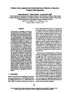
Thus, equivalent characters are organized into groups, as shown in Table 1. This strategy allows us to prepare several sets of groups, according to the requirements of a matching effort and the characteristics of source and pattern data. For instance, casesensitive groups, phonetic groups, or accent-mark-sensitive groups can be prepared and used with no code modification. Figure 1 shows examples of case- and accent-marksensitive (a) and insensitive (b) matching using the Levenshtein matrix, in the comparison of the names of two Brazilian cities, Paranaguá (PR) and Paranapuã (SP). Table 1 - Groups of characters Id L1 L2 L3 L4 L5 L6 L7
Group a, á, ã, à, ä, â e, é, è, ë, ê i, í, ì, ï, î o, ó, õ, ò, ö, ô u, ú, ù, ü, û n, ñ c, ç one group for each consonant (lowercase)
...
P a r a n a p u ã
0 1 2 3 4 5 6 7 8 9
P 1
a 2
r 3
a 4
n 5
a 6
g 7
u 8
á 9
0
1
2
3
4
5
6
7
8
1
0
1
1
2
2
3
4
4
2
1
0
1
2
3
3
4
5
3
1
1
0
1
2
3
4
4
4
2
2
1
0
1
2
3
4
5
2
3
1
1
0
1
2
2
6
3
3
2
2
1
1
2
3
7
4
4
3
3
2
2
1
2
8
4
5
3
4
2
3
2
1
Id U1 U2 U3 U4 U5 U6 U7
Group A, Á, Ã, À, Ä, Â E, É, È, Ë, Ê I, Í, Ì, Ï, Î O, Ó, Õ, Ò, Ö, Ô U, Ú, Ù, Ü, Û N, Ñ C, Ç one group for each consonant (uppercase)
...
P a r a n a p u ã
(a) fLD = 0.89
0 1 2 3 4 5 6 7 8 9
P 1
a 2
r 3
a 4
n 5
a 6
g 7
u 8
á 9
0
1
2
3
4
5
6
7
8
1
0
1
1
2
2
3
4
5
2
1
0
1
2
3
3
4
5
3
1
1
0
1
2
3
4
5
4
2
2
1
0
1
2
3
4
5
2
3
1
1
0
1
2
3
6
3
3
2
2
1
1
2
3
7
4
4
3
3
2
2
1
2
8
4
5
3
4
2
3
2
2
(b) fLD = 0.78
Figure 1 - Accent-mark-insensitive (a) and sensitive (b) edit distance
53
IX Brazilian Symposium on GeoInformatics, Campos do Jordão, Brazil, November 25-28, 2007, INPE, p. 49-60.
In the definition of the groups and in the implementation, we used the Unicode standard set of characters. Notice that most information retrieval and text mining efforts usually pre-process the input strings, eliminating uppercase characters, accent marks and other special characters. We decided not to do so, since uppercase is often used as a way to distinguish proper nouns, and since accent marks can be decisive in determining a match, depending on the language. One possible difficulty in using our method is the determination of the similarity threshold δ. We can understand more easily how to choose a value for δ if we think in terms of number of allowable errors. Considering S and P to have the same length, the maximum (integer) number of allowable errors is equivalent to ⎣(1.0 − δ ) ⋅ S ⎦ . In order illustrate that, we performed a frequency distribution analysis of word lengths in a data set containing 9,222 personal names, extracted from BDBComp (Brazilian Digital Library on Computing)2. After separating 26,924 words from names, we observe that most names have between two and four words. Almost 75% of them have between 4 and 9 characters (Table 2). The large number of 1-character words reflects the use of abbreviations in BDBComp. Therefore, using a threshold δ = 0.75, it means we allow for a maximum of one error in a 4- to 7-letter word, and 2 errors for a 8- to 11-letter word. This threshold seems adequate for personal names, and is left here as a suggestion. In our method for multiword matching, presented in the next section, this threshold applies to individual words taken separately, not to the full string. Table 2 – Frequency distribution of BDBComp name lengths and number of words Length 1 2 3 4 5 6 7 8 9 10 11 12 13 14 15 TOTAL
# names 4383 1377 469 2080 4688 4727 4638 2587 1281 426 182 52 19 8 7 26924
% 16,3 5,1 1,7 7,7 17,4 17,6 17,2 9,6 4,8 1,6 0,7 0,2 0,1 0,0 0,0 100,0
# words 2 3 4 5 6 7 8 TOTAL
#names 3894 2922 1760 553 81 11 1 9222
% 42,2% 31,7% 19,1% 6,0% 0,9% 0,1% 0,0% 100,0%
3.2 Matching multiword strings The first step for matching multiword strings is dividing them into words, using whitespace characters as delimiters, such as blanks, hyphens and other symbols. Points are preserved as the last character in the preceding word, since they can indicate abbreviations. We can also opt to preserve or to eliminate stopwords. Stopwords constitute another way to differentiate between very similar names, and therefore we prefer to preserve them in most situations. However, some sources intentionally leave them out, as in the case of names in bibliographic references, so our implementation allows treating or discarding stopwords as an option. Our matching strategy then proceeds in four phases: (1) checking for standard abbreviations, (2) checking for non-standard abbreviations, (3) word-by-word matching and (4) verifying inversions. 2
http://www.lbd.dcc.ufmg.br/bdbcomp/bdbcomp.jsp
54
IX Brazilian Symposium on GeoInformatics, Campos do Jordão, Brazil, November 25-28, 2007, INPE, p. 49-60.
First, each word in the string is tested against a list of known abbreviations. The list contains pairs of the type , where abb is the standard abbreviation (for instance, “Pres”), and val is its meaning, spelled completely (as in “President”). If an exact match is found between a word in S and an abbreviation from the list, it is replaced by its full spelling. Our intention is to expand abbreviated titles, which are quite common preceding personal names and in some kinds of place names, to their full description. We do not expect to find many false matches, i.e., words that coincide with standard abbreviations but have a meaning of their own (as in someone whose name is “Pres”). The possibility of such coincidences should be assessed by the user, who could then leave conflicting abbreviations out of the list. Next, non-standard abbreviations are verified. Candidates are 1-character capitalized words and words that end with a point. Such abbreviations are compared to each word in the pattern, and a similarity measure is then calculated as the number of matching characters of the abbreviation S [i ] divided by the number of characters in the candidate word from the pattern P[ j ] , where X [k ] denotes the kth word of string X (Eq. 3). f NSA ( S [i ], P[ j ]) =
S [i ]
(3)
P[ j ]
Unless the similarity threshold is set too low, any non-standard abbreviations in S will not find a match with regular names. We assume, heuristically, that the abbreviation has been used in order to save space or typing effort; therefore, we expect a large difference in size between the abbreviated word and its expected match in the pattern. On the other hand, it is likely that a non-standard abbreviation will reproduce the first characters from the corresponding word. We consider this case to be a match if all the characters in the abbreviated word are equal (i.e., no approximation is allowed) to the same number of characters at the beginning of the pattern word, which is where the characters that form an abbreviation are usually taken from. Even though in most cases name abbreviations involve simply an initial, with this heuristic we expect to be able to match unusual abbreviations or abbreviations that have been left out of the standard list. In the third stage, we perform word-by-word matching, using a strategy that is similar to LD calculation (Eq. 2), modified to allow for inversions and to provide a similarity measure. Our matching algorithm uses a matrix W [ S W , P W ] , where X W denotes the number of words in string X. The matrix is filled out in a row-wise traversal to the right, making Wi , j = f LD ( S [i ], P[ j ]) if S [i ] is a regular name, or Wi , j = f NSA ( S [i ], P[ j ]) , if S [i ] is a non-standard abbreviation. The value of fLD is determined using the process described in the previous section. When S [i ] is a name, after each row i is complete, we identify the column j at which the value of the similarity function is maximum. If this value exceeds the similarity threshold δ, a match exists between S[i] and P[ j ] . For the processing of the next row, the word P[ j ] is left out of the similarity comparisons if the match was exact. At the end of the process, we select the best match for each word in the pattern, considering a valid match only when (1) the similarity threshold has been reached, or (2) there is a match with a non-standard abbreviation. Denoting as v the number of matching words, we propose three similarity measures for multiword string matching. The first, fMW, is calculated dividing the sum of the similarity values found for each matching word by the number of matching words, giving an
55
IX Brazilian Symposium on GeoInformatics, Campos do Jordão, Brazil, November 25-28, 2007, INPE, p. 49-60.
idea about the average similarity of words in each string (Eq. 4). The second, fVM, indicates the fraction of the words from the pattern for which a match has been found (Eq. 5). The third measure, fINV, indicates the occurrence of inversions, and is calculated as follows. The order in which words from the string match words from the pattern is generated and analyzed, counting the number of times in which the sequence is broken. The fINV similarity is then calculated by establishing a penalty for each inversion, corresponding to the number of inversions (nI) divided by the number of matching words (Eq. 6). ⎡ SW ⎤ ( f LD ( S [i ], P[ j ]), f NSA ( S [i ], P[ j ]) )⎥ ⎢max ∑ i =1 j =1 ⎣ ⎦ f MW ( S , P ) = v v f VM ( S , P ) = max S W , P W PW
(
f INV ( S , P ) = 1.0 −
)
nI v
(4) (5) (6)
The similarity values can be used separately or combined with a weighted average. Weights are assigned according to the characteristics of the matching effort. For instance, when matching full names to bibliographic references, inversions are expected, so the inversion index can receive a lower weight than the other two measures. Equation 7 shows the calculation of the overall similarity f, where wMW, wVM, and wINV are respectively the weights for word, valid matches, and inversions, and wMW + wVM + wINV = 1 . f ( S , P) = wMW f MW ( S , P) + wVM f VM ( S , P) + wINV f INV ( S , P)
(7)
Figure 2 shows the comparison of two names, considering δ = 0.75, case- and accentmark-sensitivity. In the first row, the only the first words match, with a similarity of 0.857 (one error in seven characters). The other words from the pattern do not match the first word from the string; a similarity measure does not have to be calculated, since the comparisons fail either the length test or the bag test. Further comparisons only have to be made on “Antônio”, first word from the pattern, if an exact match has not been found. In the second row, “C.” is a non-standard abbreviation, and is compared against each word from the pattern. A match occurs with “Carlos”, for which “C.” is a possible initial. However, “Carlos” is not taken out of future comparisons, since a better match can occur with some other word. In the remaining two rows, the edit distance has to be calculated only twice. Since all words from the pattern found a match, fVM = 1.0, and fMW = 0.706, the average of the values in bold in Figure 2. Matches are in order (1