Approximation and Heuristic Algorithms for Minimum ... - Columbia CS

THE IBY AND ALADAR FLEISCHMAN FACULTY OF ENGINEERING

Approximation and Heuristic Algorithms for Minimum Delay Application-Layer Multicast Trees

A thesis submitted toward the degree of Master of Science in Electrical and Electronic Engineering

by

Eli Brosh

October 2003

THE IBY AND ALADAR FLEISCHMAN FACULTY OF ENGINEERING

Approximation and Heuristic Algorithms for Minimum Delay Application-Layer Multicast Trees

A thesis submitted toward the degree of Master of Science in Electrical and Electronic Engineering

by

Eli Brosh

This research was carried out in the Department of Electrical Engineering - Systems, under the supervision of Dr. Yuval Shavitt

October 2003

Abstract In this thesis we investigate the problem of finding minimum delay applicationlayer multicast trees, such as the trees constructed in overlay networks. It is widely accepted that shortest path trees are not a good solution for this problem since such trees can have nodes with very large degree, termed high load nodes. The load on these nodes makes them a bottleneck in the distribution tree, due to computation load and access link bandwidth constrains. Many previous solutions limited the maximal degree of the nodes by introducing arbitrary constraints. In this work, we show how to directly map the node load to delay penalty at the application host, and create a new model that captures the trade offs between the desire to select shortest path trees and the need to constrain the load on the hosts. Our model enables the evaluation of multicast performance using a single delay cost. In this model the problem is shown to be NP-hard. Therefore, we present √ a logarithmic approximation algorithm and a heuristic solution with a Ω( n) approximation ratio where n is the size of the multicast group. Both algorithms generate minimum delay trees that intrinsically balance short latency with small degree, and thus avoid an external trial-and-error type of balancing between the two, i.e., our solutions do not impose a maximum degree on the multicast trees. For overlay networks with homogenous costs, we show that the heuristic algorithm is optimal and analyze the convergence rate of a family of ’non-lazy’ multicast algorithm. Our work addressed the issue of minimum delay multicasting in the context of fully connected networks and structured topologies used by many peer-2peer systems. We show that the heuristic scheme achieves an optimal solution for grid graphs, and provide performance bounds for multicasting in grid and tree topologies. Finally, we use a simulation study to evaluate the average performance of the suggested algorithms. The simulations show that the heuristic solution is scalable for large group sizes, and produces results that are very close to optimal. The proposed solution is most useful for delay-sensitive applications, such as real-time media streaming, and can be used to provide an efficient routing infrastructure for group communication applications.

i

Contents 1 Preface 1.1 Introduction . . . . . . . . . . . . . . . . . . . . . . . . . . . . . 1.2 Background . . . . . . . . . . . . . . . . . . . . . . . . . . . . .

1 1 4

2 Overlay Communication Network Model

6

3 The 3.1 3.2 3.3

Optimal Multicast Tree Problem 8 Problem formulation . . . . . . . . . . . . . . . . . . . . . . . . 8 The optimal recursive computation . . . . . . . . . . . . . . . . 10 NP-Completeness . . . . . . . . . . . . . . . . . . . . . . . . . . 11

4 Multicast Algorithms 4.1 Approximation algorithms . . . . . . . . . . . . . . 4.1.1 The postal approximation algorithm . . . . 4.1.2 The general postal approximation algorithm 4.1.3 The MDM approximation algorithm . . . . 4.2 The heuristic algorithm . . . . . . . . . . . . . . . . 4.3 The homogenous case . . . . . . . . . . . . . . . . .

. . . . . .

. . . . . .

. . . . . .

. . . . . .

. . . . . .

. . . . . .

. . . . . .

12 12 14 15 16 19 21

5 Analysis of Specific Topologies 5.1 Motivation . . . . . . . . . . . 5.2 Trees . . . . . . . . . . . . . . 5.3 Spiders . . . . . . . . . . . . . 5.4 Grids . . . . . . . . . . . . . .

. . . .

. . . .

. . . .

. . . .

. . . .

. . . .

. . . .

. . . .

. . . .

. . . .

. . . .

. . . .

. . . .

. . . .

. . . .

. . . .

. . . .

. . . .

. . . .

24 24 25 26 27

6 A Simulation Study 6.1 Schemes compared . . . . . 6.2 Simulation results . . . . . . 6.2.1 Clique topologies . . 6.2.2 Power-law topologies 6.3 Conclusions . . . . . . . . .

. . . . .

. . . . .

. . . . .

. . . . .

. . . . .

. . . . .

. . . . .

. . . . .

. . . . .

. . . . .

. . . . .

. . . . .

. . . . .

. . . . .

. . . . .

. . . . .

. . . . .

. . . . .

. . . . .

34 34 35 35 39 39

. . . . .

7 Summary

40

ii

List of Symbols c(u, v) p(v) l(p) T V [T ] M DM M s tT (v) M (v) λuv sv U T ∆T LT γ γ0 Ui OP T n GHP IGHP OP TGHP tGHP T t[v] m[v] wu;v du;v πu;v N (t) R (t) Gm;n D b(v) d(v)

Communication delay of an edge (u, v) Processing delay of host v The cost of a path p Multicast tree Set of nodes in tree T Minimal Delay Multicast Multicast group set Source host Reception delay of host v using a multicast scheme T Optimal cost of multicasting from a subtree rooted at v Communication latency of edge (u, v) in the Postal model Switching delay of node v in the Postal model Terminal set of multicast recivers Optimal multicast tree for the postal multicasting problem Maximal generalized degree of tree T ∗ Weighted diameter of tree T ∗ Switching to communication ratio Maximal value between γ and 1 Core subset of terminals computed in the ith iteration Cost of the optimal solution for the MDM problem Multicast group size Generalized heterogeneous postal model GHP configuration instance Cost of the optimal solution for the GHP multicasting problem Reception delay of host v using a GHP multicast scheme T Ready time attribute for host v The mate host of v Weight of edge (u, v) Weight of the shortest path from u to v Predecessor of v on the shortest path from i Maximal number of hosts that can be reached in the interval (0, t] Maximal number of messages received in the interval (t − τ, t] Grid graph with size m × n Maximal distance in a grid graph Optimal broadcast time from v in a grid graph Additional delay of host v

iii

List of Figures 1.1

Examples of multicast trees . . . . . . . . . . . . . . . . . . . .

3

3.1

Example of an ordered multicast tree . . . . . . . . . . . . . . .

9

4.1 4.2 4.3

Approx-MDM cost transformation example . . . . . . . . . . . . 17 Greedy tree construction for the MDM problem . . . . . . . . . 20 √ n approximation ratio of the heuristic tree . . . . . . . . . . . 22

5.1 5.2 5.3

SPT examples for grid topology . . . . . . . . . . . . . . . . . . 29 Heuristic tree examples for grid topology . . . . . . . . . . . . . 31 Examples of B1 and B2 structures . . . . . . . . . . . . . . . . . 33

6.1

The multicast delay for a clique topology with random network costs from [1, 10] . . . . . . . . . . . . . . . . . . . . . . . . . The multicast delay for a clique topology with random processing costs from [1, 10] and unit communication costs . . . . . . The multicast delay for a clique topology with random communication costs from [1, 10] and unit processing costs . . . . . . The multicast delay for a clique topology with near homogenous random costs selected from [0.75, 1.25] . . . . . . . . . . . . . The multicast delay for a power-law topology with random network costs from [1, 10] . . . . . . . . . . . . . . . . . . . . . .

6.2 6.3 6.4 6.5

iv

. 36 . 36 . 37 . 38 . 38

Chapter 1 Preface 1.1

Introduction

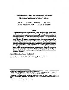
Multicast is a key component in the design of group communication applications which require efficient data delivery to multiple destinations. However, IP multicast which implements multicast functionality at the network layer is still not widely deployed in current IP networks. To alleviate this problem, several recent proposals [1] have advocated an alternative approach, termed application layer multicast or end-host multicast, which implements multicast functionality at the application layer using unicast network level services only, forming an overlay network between end hosts. The goal of application layer multicast [2] is to construct and maintain efficient distribution trees between the multicast session participants, minimizing the performance penalty involved with application-layer processing. Many proposals attempt to optimize the cost of the multicast delivery tree using application level performance metrics such as delay or throughput. The systems which aim at reducing the overall delay [2, 3, 4, 5, 6, 7] construct a minimum height (or minimum diameter) tree with constrained degrees. The degree constraints are used to control the network resource usage, i.e., available bandwidth or stress on the physical links. However, this solution stipulates the usage of a dual cost optimization objective which mixes network level and application level costs to characterize applications performance. In this thesis we advocate an application-centric approach which quantifies system performance using application level costs only. We claim that the conventional overlay network model and its corresponding delay measure are designed to characterize multicast systems which assume network-level data distribution capabilities. Unfortunately, message processing by end-hosts involves an additional delay penalty which is not captured by such models and is related to application-layer implementations of packet duplication and routing. In particular, the shift of multicast functionality to the upper level influences the simultaneous distribution capabilities of end-hosts, implying a communi1

CHAPTER 1. PREFACE

2

cation model with sequential message distribution. This constraint stems from the fundamental change in the characteristics of the routing infrastructure assumed by the overlay network, attributed to the difference between message distribution speeds of routing nodes (i.e., end-hosts) in overlay networks and packet distribution speeds of routers in conventional physical networks. For example, consider the simple network of Figure 1.1A, composed of three hosts H1 , H2 , and H3 and two routers R1 and R2 connected using a high speed backbone, where host H1 uses a low-bandwidth access link for network connectivity, e.g., modem access, and H2 , H3 use high-bandwidth LAN access connectivity. Assume that the goal of the overlay system is to devise a multicast tree that provides minimal distribution delay from H1 to H2 and H3 . Clearly, a multicast system must be careful to avoid delegating large degree to the low bandwidth host H1 in order to eliminate unnecessary bottleneck due to its low-speed data distribution capabilities. Figure 1.1B depicts the corresponding optimal multicast tree. Now, consider the conventional routing algorithm used by many application-layer multicast architectures that optimize tree delay, namely the shortest path tree algorithm. In this case the shortest path multicast tree reduces to a star topology (Figure 1.1C), which ignores the performance penalty at the star center. Hence, serialized message distribution which is irrelevant to IP multicast schemes must be accounted for in the evaluation of overlay multicast architectures. Surprisingly, however, many application-layer architectures which optimize tree delay have neglected these implications on the overall performance of group communication applications. Another factor which constrains parallel message distributions in overlay networks is the processing capacity of end-host machines. For instance, consider a server which implements router like functionality at the application layer and therefore may not have enough CPU power to handle message processing at the full speed of its network interfaces. Hence, the effective message distribution rate of an end-host is shaped by two factors, the bandwidth of the access link connecting the host or its local area network to the physical network, and the processing power and the computational load on the host machine. A recent study [8] that measured the actual end-host heterogeneity of popular p2p overly systems showed that the bandwidth and latency parameters can vary by several orders of magnitude across different hosts in the system. In this paper, we present an overlay network model which captures the realistic costs involved with application-layer multicast. The model is a mathematical generalization of a communication model developed by Cidon et al. [18] for high-speed networks, and similarly it incorporates two separate delay measures. The processing delay measure, which is a reciprocal of the effective message distribution speed of an end-host application, and the communication delay measure, which represents the delay of traversing an overlay link. This framework enables us to characterize the performance of multicast trees using

CHAPTER 1. PREFACE

3

H1

H1

R1

H2

R2

H3

H1

H3

H2

H3

H2

Low-Speed Access Link High-Speed Access Link Backbone Link

(A)

(B)

(C)

Figure 1.1: Comparison between application-layer multicast and network-layer multicast in a simple heterogeneous overlay network a single cost, the overall delay of message distribution. We use the proposed framework to develop heuristic and approximation algorithms for the problem of constructing delay optimized multicast trees. Both the heuristic and the approximation generate minimum delay trees that intrinsically balance short latency with small degree, and thus avoid an external trial-and-error type of balancing between the two, i.e., we do not impose a maximum degree on our trees. Our heuristic algorithm constructs such trees efficiently and thus can scale to large multicast groups, which is a known problem [2]. Note that the suggested solution works both for fully connected topologies, and for structured topologies, used in some p2p overlay networks [9]. Therefore, we address the issue of multicasting in partially connected networks, and provide performance bounds for tree and grid graphs. The presented algorithmic solutions can be effectively used to implement centralized overlay systems, such as p2p and server based systems. The heuristic algorithm is particularly useful in the context of two-tier server based architectures [5, 10, 3] which construct a virtual tree among the servers to provide an efficient content and data delivery services to end-users. Each end-user registers to a server in order to receive multicast services, and the server handles the dissemination of the aggregated traffic. Such semi-static architectures employ reliable servers to provide high-availability service, stipulating a simple implementation with low computational overhead due to minor topology changes. Furthermore, a centralized approach is capable of providing quick

CHAPTER 1. PREFACE

4

and efficient session management services by sharing the computational load among several overlay servers [4]. The main applicability of our algorithms is in the context of delay-sensitive multicast applications, which require tight bounds on the end-to-end delays due to jitter and timing constrains. Applications which belong to this category include audio conferencing, real-time media streaming, content distribution services, and multi-player distributed games. The rest of the thesis is organized as follows. The next chapter formulates the overlay communication model. In Chapter 3 we discuss the problem of optimal multicast tree construction and show that this problem is NP-Complete. In Chapter 4 we develop approximation and heuristic algorithms for solving this problem. Chapter 5 deals with performance analysis of the heuristic algorithm for several overlay topologies. An experimental evaluation of our solutions is presented at Chapter 6. Finally, Chapter 7 concludes our work.

1.2

Background

Broadcast and multicast are important communication primitives which have many applications in distributed and parallel systems. The problem of designing efficient broadcast and multicast algorithms under the assumption of sequential message distribution have been extensively studied in the context of several communication models. One model which was widely investigated is the telephone model [11], which assumes a synchronous communication model where each node can either send or receive a single message per communication round. Some telephone model studies have focused on the problem of designing optimal broadcast schemes for specific classes of graphs (see [12] for a comprehensive survey), while others have suggested approximations which support efficient broadcasting in general graphs ([13, 14, 20, 15]). Cidon et al. [18] presented a homogenous communication model for highspeed networks which captures communication costs using two parameters – transmission delay and computation delay. In this model, the network is represented by an undirected graph G = (V, E). Each node is associated with a processing delay cost P , and each edge is associated with a communication delay cost C. The model assumes sequential processing of messages, such that the time needed for a node to handle the transmission of i messages is iP . In addition, they proposed an optimal tree-based broadcast algorithm [18] for complete graphs, and showed that such trees achieve a broadcast delay which is logarithmic in the size of V . Raz and Shavitt [19] presented a general version of this model which supports IP-like routing, and considered efficient multicasting algorithm (based on balanced trees) for line topologies. The postal model, introduced by Bar-Noy et al. [11], is a similar homogenous model which captures network communication costs by incorporating a latency

CHAPTER 1. PREFACE

5

parameter λ. It assumes a fully connected communication model where each host can either transmit or receive a single message per time unit. More specifically, this model assumes that a message originator, u, spends one unit of time preparing and sending a message to its destination. After the transmission u is free to perform other functions including sending other messages. The destination completes the reception λ units of time after the initial preparation of the message by the originator. LogP [16] is a similar homogenous model which uses an extended set of parameters to characterize communications costs. Optimal broadcast schemes for these homogenous models can be found in [11, 17]. The heterogeneous postal model [20] extends the postal model by assuming that the communication costs are not uniform. In addition the model incorporates a switching time measure which represents the minimal gap between message transmissions. This model represents the communication network using an undirected graph G = (V, E), a switching time function which associates a sending time sv with each node v ∈ V , and a communication latency function which associates a length λuv with each pair of nodes (u, v) ∈ E. A log k approximation algorithm is given in [20] for the problem of optimal multicast where k is the size of the multicast group.

Chapter 2 Overlay Communication Network Model In this chapter we define the overlay communication model and the corresponding delay measures which characterize the performance of application-layer multicast solutions. An overlay network is a fully connected virtual network formed by hosts which communicate with each other using a physical network, such as the Internet. The physical network is composed of routing nodes (i.e., routers) and communication links. Hosts are connected to the routing nodes using access links (for example, see Figure 1.1A). The underlying assumption is that backbone links have abundant bandwidth, while access links may impose system bottlenecks due to potential bandwidth limitations. The overlay network utilizes the regular unicast services of the physical network to provide communication among hosts, and do not require any special support at the network level. The delay experienced by a message that travels between hosts is composed of two elements: I. Communication delay, which represents the delay of traversing the unicast path between the hosts. This component includes the accumulated propagation and queuing delays of the physical links on the unicast path, and the message reception overhead at the receiver host. II. Processing delay, which represents the delay of processing a message at the sender host. This element includes the overhead of preparing a message for transmission and the transmission delay through the physical access link. Although current operating systems and their communication services have mechanisms which allow applications to perform simultaneous (or near simultaneous) message transmissions, the simultaneous effect is overridden by the 6

CHAPTER 2. OVERLAY COMMUNICATION NETWORK MODEL

7

inherent serialization involved with message transmission through a physical access link. This type of serialization is typically performed at the hardware level by the access equipment. Furthermore, the sequential distribution prohibits the usage of unrealistic application design schemes which relies on simultaneous message transmissions. We define an overlay network model based on a generalization of a communication model developed by Cidon et al. [18]. The overlay network is modeled by a directed complete graph G = (V, E), where V is a set of vertices representing hosts, and E is the set of edges representing the communication paths in the overlay topology. We use the terms ”host” and ”link” to refer to the vertexes and edges in the overlay graph. Each overlay edge (u, v) ∈ E is associated with a communication delay cost, c(u, v), and each host v ∈ V is associated with a bounded and finite processing delay cost, p(v). The original model of Cidon et al. [18] assumes homogenous processing and communication costs, i.e., p(v) = P, ∀v ∈ V , and c(u, v) = C, ∀(u, v) ∈ E The direct communication between hosts is characterized as follows. Assume that at time t, host u initiates processing of a message targeted to host v. Then host u is busy processing this message during the time interval [t, t+p(u)], and the message arrives at host v at time t + p(u) + c(u, v). After this processing period (i.e., [t, t + p(u)]), host u is free to handle the following messages. Therefore, the processing delay represents the minimum time interval between consecutive message transmissions. It is important to note that in our model, the delay costs between pairs of hosts do not necessarily satisfy the triangle inequality. This is a known phenomenon in the Internet, stemming in part from policy routing. For example, Jamin et al. [21, Figures 2 and 3] show that about 30-50% of the triangles in the Internet do not obey the triangle inequality. Given a pair of hosts v1 and vk which are connected by a path pv1 ,vk =< v1 , . . . , vk > of length k − 1, the cost of the path from v1 to vk , denoted by l(pv1 ,vk ), is defined as the sum of the communication delays of the overlay links in this path and the processing delays of the traversed hosts (the processing delay of vk is excluded since it doesn’t consume processing resources for further delivery). Therefore l(pv1 ,vk ) =

k−1 X

p(vi ) + c(vi , vi+1 )

(2.1)

i=1

where vi , 1 ≤ i ≤ k denotes the ith host on the path pv1 ,vk . One may view this cost as a measure of the minimum distribution delay (using the specified path) from v1 to vk . We believe that this model captures the heterogeneity of current overlay networks, and provides a realistic framework for evaluating the performance of multicast algorithms.

Chapter 3 The Optimal Multicast Tree Problem 3.1

Problem formulation

In this chapter we state our design objective formally and show that the optimal multicast tree problem is NP-Complete. We use the term multicast scheme to refer to the task of distributing a message from a source host to a subset of hosts M in the overlay network. Since one cannot relay on the cooperation of non-participating hosts (i.e., hosts which do not belong to the multicast group M ), we assume that only the hosts in M are allowed to participate in the distribution. Thus, a multicast scheme in the graph G = (V, E) can be viewed as a broadcast scheme, i.e., the task of distributing a message to the entire network, in the subgraph induced by the host set M ⊆ V . We formulate the optimal multicast tree problem, also denoted as minimal delay multicast (MDM) problem, as follows. Definition 3.1. The optimal multicast tree problem (MDM): Given a directed complete graph G = (V, E), a multicast group M ⊆ V , a source host s ∈ M , a non-negative real processing delay p(v) for each vertex v ∈ V , and a non-negative real communication cost c(u, v) for each edge (u, v) ∈ E, find a multicast scheme which minimizes the delay by which all the hosts in M receive a message from s, namely a scheme which minimizes the arrival time of the last message. Our goal is to devise a multicast scheme which minimizes the distribution delay. Therefore, we restrict this study to non-lazy multicast schemes, in which a host that has already received a message does not delay message distribution by becoming idle (this term was introduced in [20]). Such schemes correspond to an ordered directed tree T , rooted at s and spanning M . The root of the tree corresponds to the source host s, and the 8

CHAPTER 3. THE OPTIMAL MULTICAST TREE PROBLEM

1 2 1

s 1

v1

3

v2 3

v3

v4

9

4

v5

2 4

v6

Figure 3.1: Example of an ordered multicast tree rest of the nodes corresponds to the rest of the hosts in the multicast group M . Each non-leaf node u has an ordered list of k children u1 , . . . , uk which correspond to the ordered set of k hosts u1 , . . . , uk to which host u sends the multicast message. That is, the ith outgoing edge of node u corresponds to the ith transmission from u. The reception delay of host v ∈ M , denoted by tT (v), is defined to be the time at which v receives a message from the source host, s. The reception delay of s is by definition 0. The reception delay of node v at depth k which is connected to the tree root using a unique directed path, pv0 ,vk =< v0 , . . . , vk > such that v0 = s and vk = v, is computed by summing the communication delays of the path edges and the processing delays of the traversed hosts. Therefore we have tT (v) =

k−1 X

(c(vi , vi+1 ) + p(vi ) · g(vi , vi+1 ))

(3.1)

i=0

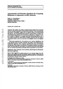
where g(vi , vi+1 ) denotes the index of the transmission from vi to vi+1 , 0 ≤ i ≤ k − 1 (i.e., the processing round number used to prepare and deliver the message from vi to vi+1 ). The cost of a multicast tree T is defined as the earliest time at which all the hosts have been notified, i.e., this cost is maxv∈M tT (v). For example, consider the ordered tree in Figure 3.1. The communications costs are located near the edges, and the processing costs near the nodes. The edges of this tree are depicted from left to right according to increasing transmission order. By applying equation (3.1) we get that the reception delay of v1 is 1 + 2 = 3. Observe that s distributes the message to v2 after two processing rounds, and therefore the reception delay of v2 is 1 · 2 + 1 = 3. Similarly, the reception delays of v3 , v4 , v5 , v6 are 7, 8, 9, 11, respectively, and the cost of the tree is 11. Given a multicast tree we can easily calculate the optimal ordering using


10

a recursive computation, working bottom-up. This recursion is presented in the following section. In the rest of the thesis we neglect the ordering and concentrate on finding the optimal tree.

3.2

The optimal recursive computation

Given a tree T = (V, E) rooted at s with associated processing and communication costs p and c, respectively, we need to compute the optimal cost and optimal ordering of T . We employ a bottom-up recursive computation approach. For each node v ∈ V, v 6= s with parent u we compute the quantity M (v). This quantity represents optimal cost of the subtree rooted at v, i.e., the minimal multicast delay from v to the nodes in its subtree. We use the quantity m(v) to incorporate the communication cost from u to v: m(v) = M (v) + c(u, v)

(3.2)

Given a non leaf node v with k children v1 , . . . , vk , we denote by r(v, i) a rank function that returns a child node of v with the ith largest m quantity. Therefore, the recursive formulation of the optimal cost of a tree rooted at a non-leaf node v is M (v) = max {m(r(v, i)) + i · p(v)} 1≤i≤k

(3.3)

The optimal cost of a tree rooted at a leaf node v is by definition m(v) = 0. The optimal multicast delay of tree T is simply M (s). The corresponding optimal ordering is computed according to the rank function, such that the ith child of a non-leaf node v is r(v, i). The time complexity of this computation is Θ(|V |). The correctness follows from the fact that in a tree graph any multicast scheme is characterized only by the message distribution order of non-leaf hosts. The following lemma provides a simple proof for the optimality of the recursive computation. Lemma 3.1. The recursive computation provides an optimal solution for minimum delay multicast in a tree graph T = (V, E). Proof. Assume to the contrary, that there exists an optimal multicast scheme in which host u ∈ V distributes a message to child hosts ui and uj in processing rounds k and l, k < l, respectively, whereas m(ui ) < m(uj ). By swapping the transmissions order to these child nodes, the multicast delay may be reduced by at most (l − k) · p(u), which contradicts the assumption that this multicast scheme outperforms the distribution order of the recursion. 2


11

Consider the example depicted in Figure 3.1. Using the recursive computation we get that M (v1 ) = max{1 + 3, 2 · 1 + 3} = 5 and M (v2 ) = max{2 + 4, 2 · 2 + 4} = 8. The optimal cost of the tree is achieved when s distributes the first message to v2 , such that the overall multicast delay, M (s), is max{1 + 9, 2 + 7} = 10. We further discuss tree graphs in Section 5.2, where we develop worst case performance bounds for multicasting in such graphs.

3.3

NP-Completeness

We now show that the MDM problem is NP-complete using a simple reduction from the telephone broadcast (TB) problem. In the Telephone model (see [11]) communication is synchronous, i.e., at each time unit a node may send a message to at most one other node. The TB problem seeks an optimal broadcast scheme which distributes a message from a source node to all the nodes in a given graph in a minimal number of time units. The TB problem is known to be NP-Hard [22, ND49] for arbitrary graphs. Theorem 3.1. The decision version of the MDM problem, finding a multicast tree with a delay bound K, is NP-complete. Proof. The problem is in NP since we can verify in polynomial time whether a certificate multicast scheme satisfies the delay bound. We prove that it is NP-Hard by a reduction from TB. Let G = (V, E) be an instance of the TB problem, and let n denote the number of nodes in V . We construct an instance of the MDM problem as follows. We form a complete graph G0 = (V, E 0 ), where E 0 = {(u, v), u, v ∈ V }, and we define the processing cost function as p(v) = 1, ∀v ∈ V , and the communication cost function as ½ 0 if (u, v) ∈ E, c(u, v) = n if (u, v) ∈ /E. We let M = V . It is easy to verify that the TB instance, represented by G, has a broadcast scheme which completes within K time units iff the MDM instance, represented by (G0 ,p,c), has a multicast scheme with a delay of K time units. 2 Note that the problem is shown to be NP-Hard when a uniform set of processing costs is considered. That is, the problem still remains hard even when using homogenous processing costs, implying that the processing cost measure is a true bottleneck for designing efficient multicast algorithms.

Chapter 4 Multicast Algorithms Since the problem of finding the optimal multicast tree is NP-complete, we seek to devise approximations and heuristics described as follows. We begin with developing approximation algorithm based on a modified version of the postal approximation algorithm. This algorithm accepts an undirected overlay graph input, implying that its domain is limited to overlay networks with symmetric links. This restriction is in many cases unrealistic due to the widespread deployment of asymmetric access links, such as ADSL and cable-modem connections. Furthermore, the approximation needs to solve multiple linear programs and therefore its running time is at least Θ(n7 ) (see [15]). We therefore devise an alternative cost-effective heuristic tree construction algorithm that supports directed overlay networks, and evaluate its performance. Finally, we analyze homogenous overlay networks where the processing and communication costs are uniform, and show that non-lazy trees achieve logarithmic multicast delay. We also discuss the extensions of these algorithms to support shared tree solutions. In the shared tree approach [23] a single tree is constructed for the purpose of multi-source multicast, such that the shared tree is used by all the group members. Our analysis show that the presented algorithms can be easily modified to support shared trees without major impact on the performance. Of course, using multiple single source multicast trees will always achieve lower delay, but at the expense of the management and resource usage overhead.

4.1

Approximation algorithms

We base our approximation on the algorithm of Bar-Noy et al. [20] originally designed for the heterogeneous postal model. The postal model represents the communication network using an undirected graph G = (V, E), a switching time function which associates a sending time parameter sv with each node v ∈ V , and a communication latency function which associates a length parameter λuv with each pair of nodes (u, v) ∈ E. In this model, the direct communication between nodes is characterized as follows [20]: assume node u sends a message 12

CHAPTER 4. MULTICAST ALGORITHMS

13

to node v at time 0 and the message arrives at v at time λu,v . The assumption is that u is free to send a new message at time su (i.e., u is considered busy – engaged only with the current transmission – in the first su time units following the previous transmission time). By definition, su is smaller than λu,v , i.e., the delay λu,v takes into account the sending time at u (and the receiving time at v). Although both models (postal and overlay) have common properties, the postal model differs from the overlay model in the following aspects. • In the postal model the communication latency of a link incorporates the sending time, while in the overlay model the sending time is incorporated in the processing delay of the sender host. Thus, the cost (i.e., delay) of delivering the ith message from u to v is the sum of the cost of (u, v) and i − 1 times the cost of u in the case of the postal model, and the sum of the cost of (u, v) and i times the cost of u in the case of the overlay model. • The postal model requires that su < λuv , ∀(u, v) ∈ E. Therefore, we need to adapt the postal approximation algorithm before applying it to the overlay model. We do this in three steps: 1. We define the generalized heterogeneous postal (GHP) model which eliminates the restriction on the values of the communication and switching (sending) measures. 2. The original postal approximation algorithm is adapted to support GHP models. This adaptation, termed general postal approximation, increases v the approximation ratio by a multiplicative factor γ = max(v,w)∈E { λsvw } 3. We construct a cost preserving transformation from the overlay model to the GHP model and apply the general postal approximation to compute the multicast tree. This process results in an approximation algorithm, Approx-MDM, which increases the original approximation ratio by an additive factor. We now proceed to define the GHP model. Definition 4.1. The GHP model is a heterogeneous postal model which excludes the restriction on the network costs, such that the edge length parameter in the GHP model is finite and positive, i.e., λuv > 0, ∀(u, v) ∈ E. Therefore, in the GHP model the communication latency between nodes can have any finite positive real value, providing a framework that includes nodes with switching time which is larger than the communication latency to the neighbors. The following measure captures the proportion between switching and communication times.


14

Definition 4.2. Given a GHP model with graph G = (V, E), switching time v function s, and a communication latency function λ, define γ = max(v,w)∈E { λsvw } as the switching to communication ratio of the graph G. Before proceeding to the general postal approximation we provide an outline of the postal approximation algorithm. The interested reader is directed to [20] for the full details. In the context of the postal model the multicast problem is defined as follows. Given a configuration of an undirected graph with associated communication and switching cost functions (G = (V, E), s, λ), a set of terminals U ⊆ V , and a source node r ∈ U , find the minimal time (i.e., delay) scheme that distributes a message from r to the terminal set U , where all the nodes in V may participate in the distribution. Observe that we preserve the notations of [20] which denote the multicast group by U .

4.1.1

The postal approximation algorithm

The basic idea of the algorithm is to find a multicast tree T which minimizes the quantity ∆T + LT , where ∆T denotes the maximum generalized degree (the actual degree multiplied by the corresponding switching time) of T , and LT denotes the maximum distance (in T ) from r to any of the nodes in U The algorithm computes a multicast tree, which approximates the cost of the optimal tree, T ∗ , iteratively using l rounds. Let Ui denote the terminal set in the ith round. The algorithm starts with the initial set U0 = U and terminates when U` = {r}. In the ith round the algorithm uses the core procedure to compute the following, for any i ≤ l: 1. a core subset Ui ⊆ Ui−1 of size at most

3 4

· |Ui−1 | where r ∈ Ui

2. a multicast scheme from Ui to Ui−1 , such that the obtained multicast time is linear in the optimal multicast time from r to Ui−1 . The computation of core(Ui ) involves the following steps: 1. Solve a linear program, variant of a multicommodity flow. The resulting set of fractional paths is rounded [20, Theorem 4] producing a set of |Ui | integral paths, one for each terminal. The length and congestion properties of the integral paths are linear in ∆T ∗ + LT ∗ . The congestion property is the generalized degree of the graph spanned by a set of paths. 2. Transform the set of paths into a set of spider graphs, which are graphs where at most one node has a degree larger than two. The resulting spiders span at least half of the nodes in |Ui |. Each spider contains at least two terminals, and its generalized degree and diameter is linear in ∆T ∗ + LT ∗ .


15

3. Select an arbitrary terminal from each spider together with nodes which are not spanned by any spider to be included within the resulting core. This selection ensures that the chosen spider terminal is able to distribute a message to the remaining spider nodes in O(∆T ∗ + LT ∗ ). In [20] it is shown that the resulting tree has a O(log |U |) multiplicative approximation factor. The postal approximation algorithm cannot be directly applied to the GHP model due to the particular selection of the coefficients of the rounding matrix. The following section describes the new rounding matrix used to derive the general postal approximation algorithm.

4.1.2

The general postal approximation algorithm

We now describe the GHP rounding matrix which enables the support of networks with γ ≥ 1, i.e., GHP models. We preserve the notations of [20], P1 , P2 , . . . denotes the length bounded fractional flow paths, and V (Pi ) and E(Pi ) denotes the set of nodes and edges in a path Pi , respectively; f (Pi ) denotes the amount of flow pushed on path Pi , and P j denotes the set of all paths that carry flow of the jth commodity. To simplify the presentation of the results we define γ 0 = max{1, γ}. In the general postal approximation, the following rounding matrix (termed GHP rounding matrix) is used for rounding the fractional solution of step (1) in the core computation. X f (Pi ) ≤ 6∆T for each v sv · i: v∈V (Pi )

for all j

0

−4LT · γ ·

X

f (Pi ) = −4LT · γ 0

i: Pi ∈P j

The sum of positive entries in the ith column is: X X sv ≤ λvw · γ 0 + stj ≤ 4LT · γ 0 . v∈V (Pi )

(v,w)∈E(pi )

where the second part of the equation follows from the definition of γ. The sum of the negative entries at each column is at most −4LT · γ 0 . By invoking the rounding theorem [20, Theorem 4] we get a set of integral paths such that their congestion is at most 6∆T ∗ + 4LT ∗ · γ 0 and the length of each path is at most 4LT ∗ · γ 0 . The general postal approximation algorithm. The general postal approximation algorithm is a postal approximation algorithm which employees a GHP rounding matrix instead of the original one.


16

The correctness of the modified algorithm follows from the fact the algorithm structure and its underling theorems and lemmas are not related to the specific switching and communication cost values, except of the constrained selection of the rounding coefficient which we handle appropriately. Therefore it remains to show the approximation ratio. The transformation performed on the rounded paths, step (2) in the core procedure, yields a set of spiders, such that the diameter of each spider is at most 4 · γ 0 · (∆T ∗ + LT ∗ ) and the generalized degree (of the center) of a spider is at most 6 · γ 0 · (∆T ∗ + LT ∗ ). Since the algorithm invokes O(log |U |) iterations of the core procedure and the cost of the optimal tree T ∗ is at least 0.5 · (∆T ∗ + LT ∗ ) [20, Lemma 1], we have that the multicast time from the root r to a set of terminals U is at most O(log |U | · max{1, γ}) times the optimal multicast time.

4.1.3

The MDM approximation algorithm

The following is a polynomial algorithm that approximates the minimum multicast delay. The algorithm accepts as an input an overlay network configuration, (G, c, p), which consists of an undirected graph G = (M, E 0 ) with associated processing and communication cost functions, p and c, respectively, and a source host s˜ ∈ M . Given an overlay network graph (V, E), the input graph, G, is the subgraph induced by the multicast group set M ⊆ V (see Section 3.1).

Algorithm Approx-MDM(˜ s, G, p, c) 1. Construct a GHP configuration instance IGHP = (G, s, λ), from the graph G, switching time function sv = p(v), ∀v ∈ M and communication latency function λu,v = c(u, v) + (p(u) + p(v))/2, ∀(u, v) ∈ E 0 . 2. Invoke the general postal approximation to compute a multicast tree using IGHP , source host s˜, and multicast group U which spans M , i.e., U = M. 3. Return the computed multicast tree An example of the cost transformation performed in step (1) of the ApproxMDM algorithm is presented in Figure 4.1. The input instance (see Figure 4.1A) is a simple overlay network with three hosts. The corresponding GHP network is presented in Figure 4.1B. The algorithm runs in polynomial time due to the polynomial time construction performed is step (1) and the polynomial execution time of the approximation algorithm in step (2). The correctness of the algorithm follows immediately from the correctness of the general postal approximation algorithm.


17

p1 c1

p3

p1= s1 c2

l1=

p2

c3

(A)

p + p2 c2 + 1 = l2 2

p1 + p3 + c1 2

p3= s3

p + p2 c3 + 3 = l3 2

p2= s2

(B)

Figure 4.1: Example that illustrates the cost transformation of the ApproxMDM algorithm (A) The overlay instance (B) The resulting GHP instance The following lemma shows the approximation ratio of the algorithm. Let OP T denote the multicast delay of the optimal tree and let n denote the size of M . Let pmax = maxv∈M p(v) and pmin = minv∈M p(v) be the maximal and minimal processing costs of the hosts in M . Theorem 4.1. The multicast delay of the Approx-MDM algorithm is at most (OP T + (pmax − pmin )) · O(log n) GHP

Proof. Given a multicast tree T which spans M and a host v ∈ M , let tT (v) be the reception delay of v assuming GHP timing. Similarly to equation (3.1), the GHP reception delay of v is GHP

tT

(v) =

k−1 X

(λvi ,vi+1 + svi · (g(vi , vi+1 ) − 1))

(4.1)

i=0

where vi , 0 ≤ i ≤ k − 1, v0 = s and vk = v, denotes the ith host on the unique directed path in T from s to v, and g(vi , vi+1 ) denotes the index of the transmission from vi to vi+1 . Observe that, due to the definition of the postal model (see Section 4.1), there is a delay gap of a single processing round (per each traversed host) between the message delivery delays in the postal and overlay models. By substituting the computed switching and communications costs of IGHP with the corresponding overlay input costs, i.e., sv = p(v), λu,v = c(u, v) + (p(u) + p(v))/2, we get the following relationship between the reception delay costs. p(s) − p(v) GHP + tT (v) (4.2) tT (v) = 2 Now, consider the following quantities which are computed assuming GHP ∗ timing model. Let OP TGHP be the multicast delay of an optimal tree TGHP for


18

the IGHP configuration. Let u ∈ M be the node with the maximal reception ∗ delay in TGHP . Therefore we have that OP TGHP ≤ OP T +

p(u) − p(s) pmax − pmin ≤ OP T + 2 2

(4.3)

where the first inequality follows from Equation (4.2) and the second one follows from the substitution of p(u), p(s) in equation(4.3) with pmax , pmin . The constructed IGHP instance satisfies γ < 2, since p(v) < 2, ∀(v, w) ∈ E 0 0.5 · (p(v) + p(w)) + c(v, w)

(4.4)

The constant bound on γ implies that the multicast delay of the resulting tree is at most OP TGHP ·O(log n). Substituting OP TGHP according to equation (4.3) gives the requested upper bound for the multicast delay. 2 When the processing costs are all equal, it improves our approximation for the MDM problem to O(log n). We do not restrict the communication costs to be homogeneous. The following theorem handles this case. Theorem 4.2. Consider an overlay model with homogenous processing costs, i.e., p(v) = p, ∀v ∈ V . The multicast delay of Approx-MDM algorithm for this case is at most OP T · O(log n) Theorem 4.2 can be obtained by substituting pmax = pmin = p in Theorem 4.1. Given a network with symmetric communication costs, a multicast tree T rooted at s can be easily adapted to support multicasting from multiple sources. To enable the multicast from a host v ∈ M, v 6= s, we reverse the direction of the edges on the path from s to v. This modification results in a multicast scheme with a delay which at most p(v) − p(s) + 2 · C

(4.5)

where C denotes the cost of T . Therefore, the undirected version of T can be used as a shared tree such that the multicast delay of any host v = 6 s is at most 2 · (OP Ts + (pmax − pmin )) · O(log n) (4.6) where OP Ts denotes the optimal multicast delay from s.


4.2

19

The heuristic algorithm

We introduce a heuristic tree construction algorithm which solves the directed variant of the MDM problem. The proposed algorithm computes the multicast tree incrementally using a greedy approach; for each host not yet included in the tree, the algorithm computes its minimum reception delay, and the host with the maximal delay quantity is selected. The tree is extended with the hosts on a minimum delay path between the selected host and a notified host. Figure 4.2 shows the steps of the algorithm. The input to this algorithm is the same as the input to the Approx-MDM, except for the source host which is denoted by s. The algorithm maintains a ready time attribute t[v] for each host v ∈ M which records the minimal time at which the host is free to initiate processing of a new message. The ready time is set to infinity to indicate non notified host. The constructed tree is denoted by T and the corresponding set of notified hosts by V [T ]. In each iteration, the algorithm determines for each host u ∈ M − V [T ] its mate host m[u] ∈ V [T ] by selecting a path which minimizes the ready time attribute of u, setting v to indicate the host with the maximal reception delay. Then, it updates the ready time of the hosts on the path from m[v] to v to reflect the processing time involved with delivering a message to a newly notified host v, and it adds the path hosts to the constructed tree T . The variable w indicates the current updated host. The algorithm terminates when all the hosts are notified. To be able to calculate the connection cost between a non notified host and a notified host, a preprocessing phase of computing all pairs shortest path using the Floyd-Warshall algorithm [24] is implemented. Given a pair of hosts v1 and vk connected P by a path < v1 , . . . , vk > of length k − 1, the cost of this path is defined as k−1 i=1 p(vi ) + c(vi , vi+1 ), where vi , 1 ≤ i ≤ k denotes the ith host on this path, i.e., this cost represent the minimal distribution delay (along the specified path) from v1 to vk . A shortest path from host u to host v is defined as any path between these hosts with minimum cost. Therefore, the input to the Floyd-Warshall computation is an n × n weight matrix W = (wvi ,vj ) defined as: ½ p(vi ) + c(vi , vj ) if vi 6= vj , wvi ,vj = (4.7) 0 otherwise . where n denotes the size of M . The output of the all pairs shortest path computation is composed of two n × n matrices; all pairs distance matrix D = (dvi ,vj ) and predecessor matrix Π = (πvi ,vj ); where dvi ,vj stores the weight of the shortest path from vi to vj , and πvi ,vj stores the predecessor of vj on its shortest path to vi assuming that such a path exists, otherwise πvi ,vj stores a null pointer. Observe that the shortest path from the source s to any host v is a lower bound on the cost of the optimal tree. This algorithm can be extended to support a shared tree solution using


Algorithm Heuristic-MDM(G, p, c, s) 1. t[s] = 0, set s as the root of a tree T 2. for each v ∈ M − {s} 3.

do t[v] ← ∞

4. for each (u, v) ∈ E 5.

do wu,v = c(u, v) + p(u)

6. for each (u, v) ∈ /E 7.

do if v = u then wu,v = 0 else wu,v = ∞

8. D, Π ← All-Pairs-Shortest-Path(G, W ) 9. while M − V [T ] 6= ∅ 10.

for each host u ∈ M − V [T ] do

11.

m[u] ← arg minv:v∈V [T ] {t[v] + dv,u }

12.

v ← arg maxu:u∈M −V [T ] {t[m[u]] + dm[u],u }

13.

w←v

14.

while w 6= m[v] do

15.

t[w] ← t[m[v]] + p(w) + dm[v],w

16.

add w to T as a child of πm[v],w

17.

w ← πm[v],w

18.

t[m[v]] ← t[m[v]] + p(m[v]), t[v] ← t[v] − p(v)

19. return T Figure 4.2: Greedy tree construction for the MDM problem

20


21

the following modification. At the initialization phase the longest path in the graph G is computed using the weight matrix W , and the hosts on this path are used as the initial set of notified hosts in T . The shared tree variant uses this initial selection instead of the original one and proceeds with normal tree construction as in the original algorithm. The complexity analysis of this algorithm is straightforward. The all pairs shortest path computation requires Θ(n3 ) time. Each iteration requires O(n) time to find a single mate host, and O(n) time to extend the tree. The total time per iteration is therefore O(n2 ), and the total running time of the heuristic algorithm is Θ(n3 ). We conjecture this time complexity cannot be improved since any algorithm should at least calculate the all pair shortest path. We show using an example (see Figure 4.3A) a lower bound on the approximation ratio of the heuristic tree. Consider the following complete undirected graph G = (V, E) with n + 1 hosts denoted by v0 , . . . , vn , with processing costs defined as p(v) = 1, ∀v ∈ V , and communication costs c(vi , vj ) defined as   0 if i = 0, j = 1, . . . n , δ if 1 ≤ i ≤ n − 1, j = i + 1 , c(vi , vj ) = (4.8)  n otherwise . where δ → 0. For the simplicity of presentation Figure 4.3A omits the edges with cost n. Assume that the source host is v0 and that M = V . Therefore, the heuristic scheme would have v0 distribute the message to the rest of the hosts using n processing rounds, such that the tree cost is n (see Figure 4.3B). On the other hand, consider an improved scheme in which v0 distributes the message to k hosts, and the last host in the graph receives the message in k + mδ time units, where m is a positive integer. Let |pi | denote the length (i.e., the number of edges) of path pi . Such a scheme can be obtained by a tree composed of k paths p1 , . . . , pk which share only single host, v0 (i.e., only v0 has an out-degree more than two), and the lengths of these paths form the following non increasing sequence: |pi | − 1 = |pi+1 |,1 ≤ i ≤ k − 1, whereas for a single index j in this set we may have |pj | = |pj+1 |. Figure 4.3C depicts such a tree when n = k·(k+1) . Assume that v0 distributes the message to these paths 2 (i.e., to its k children in the tree) according to a decreasing path length order. Therefore, the cost of the optimal tree is less than (1 √ + δ) · k. Since the set of paths √ span all the hosts in V we have that k = O( n), and therefore we get Ω( n) approximation ratio for the multicast delay. We conjecture that this example represents the worst case, namely that our heuristic algorithm is an √ n-approximation.

4.3

The homogenous case

Consider a fully connected overlay network with homogeneous processing and delay costs, i.e., p(v) = p, ∀v ∈ V , c(u, v) = c, ∀(u, v) ∈ E. We denote this


d

v0

v0

0

v1

22

0 0

v2

d

0

vn

vn vn-2

v1

v3

vn-1

(A)

v2

v0

vk

v1

vn (C)

v2

v3 (B)

√ Figure 4.3: Example that provides n approximation ratio for the heuristic tree. (A) The input graph (B) The heuristic tree. (C) An improved tree. model as the homogenous overlay network. In the homogenous overlay network, a non-lazy scheme directs each notified host to distribute the multicast message to a new host every processing interval p. Due to symmetry, any non-lazy multicast algorithm which avoids sending duplicate messages to the same destination host will result in an optimal solution. In particular, an optimal solution can be obtained by using the non-lazy centralized Heuristic-MDM algorithm described in Section 4.2. In this case, at each iteration the heuristic algorithm arbitrarily selects a non-notified host and then it connects this host to the notified set using a single overlay link. Next we analyze the convergence rate of message distribution in the homogeneous overlay network. In this analysis we assume that M = V , i.e., we handle the case of broadcasting. We remark that in [18] Cidon et al. showed that a tree-based broadcast provides a logarithmic delay. They have also provided a recursion (that describes the convergence rate of broadcasting) similar to ours. However, their results were derived using different techniques than ours, and therefore in the following we present our new techniques for deriving the required convergence rate. We define N (t), for t ≥ 0, as the maximal number of hosts that can be reached during the time interval (0, t], and define Rτ (t), for t ≥ τ , as the maximal number of multicast messages received during a time interval (t−τ, t]. The following lemma provides the relationship between these two functions. Lemma 4.1. In the homogenous model, the maximal number of hosts that can be reached during the time interval (0, t − c] is equal to the maximal number of multicast messages received during the time interval (t, t + p], i.e. N (t − c)=Rp (t + p), for all t ≥ c.


23

Proof. Clearly, Rp (t + p) is equal to the maximal number of messages which their processing was initiated in the interval (t − p − c, t − c]. Each host can send only a single message during an interval of length p, resulting in a one-toone correspondence between transmitted messages and hosts. The messages initiated in the interval (t − p − c, t − c] are distributed by two types of hosts: those that have completed their message processing in the interval and newly notified hosts which received a multicast message within the interval’s time. Let Y be the maximal set of hosts which have finished their message processing in the interval (t−p−c, t−c], and let X be the maximal set of hosts which were notified at that same interval. Therefore, we have Rp (t + p) = |X| + |Y |. Since each host which was notified in the interval (0, t − p − c] initiates a single new message in the interval (t − p − c, t − c] we have |Y | = N (t − c). Consequently, we get the desired relationship Rp (t + p) = N (t − p − c) + |X| = N (t − c), for any t ≥ τ . 2 Using the previous Lemma we show that N (t) can be calculated recursively. Theorem 4.3. In the homogenous model, the maximal number of hosts that can be reached during the time period (0, t] is given by ½ 1 if 0 ≤ t < p + c, N (t) = N (t − p) + N (t − p − c) if t ≥ p + c. Proof. From the definition of the homogenous overlay model, we have N (t) = 1, for 0 ≤ t < p + c. The difference between N (t) and N (t − p), for any t ≥ p, is equal to the maximal number of hosts that were notified during the interval (t − p, t], which by the definition of the Rτ function, is Rp (t). Therefore, using lemma 4.1 we have that N (t) = N (t − p) + N (t − p − c), for t ≥ p + c. 2 Since N (t − p) ≥ N (t − p − c) for any t ≥ p + c, we can derive the following upper and lower bounds of the function N (t): t

t

2b p+c c ≤ N (t) ≤ 2b p c

(4.9)

for any real numbers t, p, c ≥ 0. These bounds imply that the optimal algorithm has a logarithmic delay in homogeneous overlay networks.

Chapter 5 Analysis of Specific Topologies 5.1

Motivation

In this chapter we address the issue of multicasting in partially connected overlays, and analyze the performance bounds of degree constrained trees assuming a general family of non-lazy multicast algorithms. We also check the applicability of our heuristic algorithm for common structured overly graphs such as spiders and grids. Partial overlay connectivity, which utilizes arbitrary or structured graphs as the underlying overlay topology, is an important model which arises in several contexts. Partial connectivity is implemented by many data distribution services, such as content distribution networks and multimedia streaming systems, which utilize a dedicated network of leased lines and virtual connections to provide connectivity among application servers. These systems optimize resource usage, e.g., network bandwidth and computational overhead, and therefore enforce connectivity constrains to achieve efficient resource utilization. Structured p2p systems [9] is another class of applications which utilize partial connectivity overlays. Despite the fact that many of these systems employ distributed architectures, our centralized application-centric approach can still be used to provide theoretical performance bounds on the multicast delay in such systems. Partial connectivity may also rise in cases where due to anonymity requirements not all the hosts are aware of each other and thus connectivity is sparse. That is, hosts use local policies to override universal connectivity. For example, consider security policies in the internet, which limit the connectivity of hosts located behind firewalls and NAT facilities. Partial topologies are also relevant to the case of active networks [19], which have similar properties to those of overlay networks. It is possible to view the overlay network as an application level implementation of the active network model, where the active network uses programmable routers to add new functionality and services to the network. For example, Raz and Shavitt 24

CHAPTER 5. ANALYSIS OF SPECIFIC TOPOLOGIES

25

[19] have used a framework that considers the processing and communication delays in active networks, to develop and analyze the time complexity of several basic algorithms, including multicasting. Their framework uses the processing delay measure to capture the delay imposed by a software router implementing copy and forward of packets. Therefore, in order to support networks with partial connectivity an extended overlay model is assumed; in this model the communication cost of an overlay link (u, v) is set to infinity, i.e., c(u, v) = ∞, to indicate the absence of direct communication from u to v. For general graph topologies our analysis focuses on the performance of the broadcasting communication primitive in which a source host disseminates a message to the rest of the hosts in the graph. In the next sections, we provide performance bounds for several common undirected graph topologies.

5.2

Trees

We consider broadcasting in tree graphs. In these graphs each node has a single path from the root, implying that any broadcast scheme is characterized only by the message distribution order of non-leaf hosts. The following lemma shows that any non-lazy algorithm achieves a constant approximation factor equivalent to the maximal degree in the tree. Lemma 5.1. Any non-lazy broadcast scheme provides a factor d approximation for the minimal broadcast delay for a tree graph T with a maximal degree of d. Proof. Denote by s the source host. We use the path cost notation defined in Section 2, i.e., the cost of a path represents the minimal distribution delay along it (see equation (2.1)). In any (non-lazy) broadcast scheme the delay by which the last notified host, denoted by v, receives a message is composed of two quantities, the cost of the path from s to v, and the sum of the additional processing delays invoked by the hosts on this path (the additional delay of v is assumed to be zero). By definition, the former quantity is no more than OP T , where OP T denotes the optimal broadcast delay. We denote by < v1 , . . . , vk > the path of length k − 1 which connects between s and v, such that v1 = s and vk = v. Due to the bound on the degree of the tree, each node may delay the processing by at most d − 1 processing rounds, Pand therefore the sum of the additional processing delays is at most (d − 1) · k−1 i=0 p(vi ), where vi , 1 ≤ i ≤ k denotes the ith host on the path from s to v. It is easy to see that this quantity is at most (d − 1) · OP T , and the lemma follows. 2 This result indicates that a distribution along a degree-constrained multicast tree at an arbitrary order, such as delivery schemes used by overlay multicast systems which ignore sequential distribution of messages, produces


26

a delay which is up to a multiplicative constant factor higher than the optimal result. The heuristic algorithm achieves optimal solution for a special class of tree graphs termed spiders. We discuss these graphs in the following section.

5.3

Spiders

Spider graphs are a special class of tree graphs in which at most one node, the spider center, has degree larger than two. To simplify the analysis we ignore degenerate structures which lack a central node. The center host has a single unique path to each leaf, and therefore any broadcast scheme can be characterized by the order of message distribution from this host. The next lemma indicates that the heuristic algorithm produces an optimal distribution based on a decreasing path cost order. Lemma 5.2. The Heuristic-MDM algorithm provides an optimal broadcast scheme for a spider graph G = (V, E) with a source, s ∈ V , which is a leaf or a center host. Proof. We use the path cost notation defined in Section 2, i.e., the cost of a path represents the minimal distribution delay along it (see equation (2.1)). We begin with the case where s is a center host. Assume that G contains n leaves, vi , i = 1, . . . , n sorted according to the costs the paths which connect them to s. Denote the corresponding path set by {ps,vi }ni=1 , such that we have l(ps,vi ) ≥ l(ps,vj ) when i < j, for any 1 ≤ i, j ≤ n, where l(ps,vj ) denotes the cost of path ps,vj . It is easy to see that our heuristic performs the message distribution from s to the n paths ps,vi , i = 1, . . . , n (i.e., distributes the message to the n children of the source) using a decreasing path cost order, such that the first message is distributed to the host on ps,v1 and the last to the host on ps,vn Assume on the contrary, that there exists an optimal broadcast algorithm in which s distributes a message to paths ps,vi and ps,vj in processing rounds k and l, such that k < l and l(ps,vi ) < l(ps,vj ). By swapping the order of message delivery to these paths, the broadcast delay is maintained or reduced by at most (l − k) · p(s), which contradicts the assumption that this broadcast scheme outperforms the distribution order of the Heuristic-MDM algorithm. The case of broadcasting from a leaf host is similar and therefore the proof is omitted. 2 Observe that the worst case broadcasting from the center host, s, is attained when message distribution is performed in increasing path cost order, such that the path with the maximal cost is notified last. This scheme has a delay of lmax + (deg(s) − 1) · p(s)

(5.1)


27

where deg(s) denotes the out-degree of s, and lmax denotes the maximal cost of a path connected to s. Clearly, the optimal broadcast delay OP T is greater than lmax and greater than (deg(s) − 1) · p(s). Hence, 1 OP T ≥ (lmax + (deg(s) − 1) · p(s)) 2

(5.2)

Therefore we have that the broadcast delay of any non-lazy solution in a spider graph is, at most, a factor two of the optimal.

5.4

Grids

This section investigates broadcasting in the context of homogenous rectangular grid graphs. Let Gm,n = (V, E) denote an m × n grid graph. Each node in this graph is uniquely identified by a row and a column indices (i, j), where 1 ≤ i ≤ m and 1 ≤ j ≤ n. The broadcast analysis is conducted assuming a homogenous communication model where p(v) = 1, ∀v ∈ V and c(u, v) = 0, ∀(u, v) ∈ E. This particular selection reduces the model to the well known telephone model, and enables the usage of known results in grid broadcasting. The problem of finding an optimal broadcast scheme in 2-dimensional grid graphs have been previously investigated by Farley and Hedetniemi [25]. They have shown that: Given a grid graph Gm,n with a node v at position (i, j). Then  = n+1  D + 2 if i = j = m+1 2 2 m+1 D + 1 if i = 2 or j = n+1 , i 6= j b(v) = 2  D otherwise. where b(v) denotes the optimal broadcast time (i.e., delay) from v, and D denotes the maximal distance from v to a corner node in Gm,n . The distance between a pair of nodes u and v in positions (iu , ju ) and (iv , jv ), respectively, is defined as the number of edges on the shortest path between them, i.e., ||u − v|| = |iu − iv | + |ju − jv |. Next, we show that the shortest path tree produces a near optimal solution for broadcasting in grid graphs. Let OP T denote the cost of an optimal solution for broadcasting in grid graphs. Theorem 5.1. The broadcast delay of a shortest path tree for homogenous cost grid graph Gm,n = (V, E) is at most OP T + 2


28

Proof. Let s denote the source host, and let T denote a directed shortest path tree (SPT) rooted at s. The SPT structure implies the following degree delegation in T . If s is a corner host (one of the hosts (1, 1),(1, n),(m, 1),(m, n)) then its degree is 2 and the rest of the hosts have maximal out-degree of 2. If s is a side host (any host located at (k, 1),(k, n),1 < k < m or (1, l),(m, l),1 < l < n) or interior host (any host located at (k, l),1 < k < m,1 < l < n), then the maximal out-degree of the interior hosts which share a common coordinate with s is 3 and the maximal out-degree of the rest of the hosts is 2. The degree of s is 3 when s is a side host, and 4 when it is an interior host. Let S3 denote the set of hosts in V \ {s} such that the out-degree of these hosts in T is 3, i.e., S3 = {v : deg(v) = 3, v 6= s} where deg(v) denotes the out-degree of v in T. Let T2 be a binary subtree of T rooted at r, such that r is a child of v ∈ S3 or a side host which is a child of s. The grid topology implies that a subtree of height d, rooted at an internal node of T2 , has a single leaf at depth d. Therefore, by using the bottom-up recursive computation of Section 3.2 we get that the optimal broadcast delay from the root of a T2 tree with height d is d. If s is a corner host then T has two T2 subtrees linked to it (that is, the root of each subtree is a child of s). Since only one of these trees has a height of D − 1 while the height of the other is at most D − 2, the broadcast delay from a corner host is D, and the lemma follows for this case. The other cases are analyzed using a compressed version of T . A T2 tree with height d can be ’compressed’ to a path with d edges which preserve the broadcast time of the tree. The compressed version of T , denoted as Tc , is produced by replacing all the T2 subtrees with their corresponding paths. This compression does not modify the broadcast time of T . Let T3 denote a subtree in Tc rooted at a child of s. The topology of this subtree can be one the following: a line, a spider where the spider center is a side host of out-degree 2, or a trinary tree (i.e., trees which contain at least a single host with out-degree 3). Next, we consider the case of trinary T3 trees. The grid topology implies that a subtree of height d rooted at an internal node of T3 , v ∈ S3 , may have at most two leaves at depth d. Each host v ∈ S3 has three children in T , v1 ,v2 and v3 , ordered according to the height of the subtrees rooted at these hosts, such that h(Tv1 ) ≤ h(Tv2 ) ≤ h(Tv3 ) where Tvi ,i = 1, 2, 3 denotes the subtree rooted at vi , and h(Tvi ) denotes the height of Tvi . Given a subtree of height d rooted at v with a single leaf at depth d, the grid topology implies that h(Tv3 ) > max{h(Tv2 ), h(Tv1 )} (5.3) If the subtree has two leaves at depth d, then h(Tv3 ) = h(Tv2 ) > h(Tv1 )

(5.4)

By using a bottom-up recursive computation we get that the broadcast


(A)

29

(B)

Figure 5.1: Examples that illustrate two SPT broadcast schemes in a 7 × 5 grid; source host is colored in black (A) Near optimal tree (B) An optimal tree delay from the root of a T3 tree with height d is at most d + 1 when there is a single leaf at depth d, and at most d + 2 when there are two leaves at depth d. If s is a side host, the root of T is linked with three T3 subtrees. If s is a middle side host, i.e., a host with coordinate (is , js ) such that is = m+1 or 2 n+1 js = 2 , there are two hosts at distance D from s. If these two hosts reside in the same T3 tree, then the maximal height of the remaining T3 trees is D − 2 and we have that the broadcast delay from a corner host is at most D + 2. If these two hosts reside in different subtrees, then the maximal height of the third subtree is D − 2 and the broadcast delay is again at most D + 2. In the case of a non middle side host, the single host at distance D is located at one of the T3 trees and the maximal height of the remaining trees is D − 2, and therefore the broadcast delay is at most D + 2. Therefore, the lemma follows for this case. If s is a interior host then T has four T3 subtrees linked to it. By checking all the possible combinations it can be easily shown that the broadcast delay from an interior host is at most OP T + 2. 2 Figure 5.1 shows two shortest path tree broadcast schemes in a 7 × 5 grid graph. The source host is located in the middle of the grid. Figure 5.1A shows the worst case SPT scheme which achieves a delay of 9 time units, and Figure 5.1B shows an optimal SPT scheme which achieves a delay of 7 time units. The following lemma shows that the heuristic algorithm builds an SPT which provides an optimal solution. For the simplicity of the analysis, we assume that the heuristic algorithm uses a tie-breaking strategy to handle multiple path choices when connecting a new non-notified host to the partially constructed tree. This strategy selects paths which satisfy the following


30

properties. I. The path has the minimal cost among all the paths leading to the constructed tree II. The path uses the minimal number of direction changes in the grid topology. This strategy greatly simplifies the analysis, since it implies that the algorithm uses one-turn paths, i.e., paths with only one direction change, or zero-turn paths, i.e., horizontal or vertical paths. Lemma 5.3. The tree constructed by the Heuristic-MDM algorithm is a shortest path tree. Proof. Let s denote the source host. Let T be the partial tree constructed by the algorithm and let V [T ] be the set of hosts in T . Let d(u) be the difference between the ready time of a non notified host u ∈ V [T ] and its distance from s, such that d(u) = t[u] − ||u − s||. We denote this quantity as the additional delay of host u. We denote the first path which the algorithm connects to s as p1 , and the second one as p2 . Let V (p) denote the set of hosts in path p. Given a one-turn path p =< v0 , . . . , vk >, we define the induced set of p to be the rectangular set of hosts bounded by p and p∗ , where p∗ denotes the alternate one-turn path which connects v0 to vk . We assume that the induced set includes the hosts in V (p∗ ) and V (p). We divide the analysis to the following cases. First, we consider broadcasting from a corner host. After the first iteration, the hosts in p1 offers the lowest reception delay to all the non-notified hosts in the rectangular set induced by this path. Let S1 be the set of hosts located on the grid side adjacent to a corner host v1 ∈ V (p1 ), v1 6= s. In the following iterations, the algorithm connects non-notified hosts from S1 according to a decreasing distance order from s. Each such host is connected by a zero-turn path to its closest host in p1 . This construction ensures an SPT structure. An example of such broadcast tree in a 7 × 5 grid graph is depicted in Figure 5.2A. Next, we consider broadcasting from a side host. Assume that p1 doesn’t contain interior hosts. Prior to connecting p2 the behavior of the algorithm is similar to its behavior in the case of broadcasting from a corner host. Thus, it connects non-notified hosts from S1 to their closest host in p1 . After the iteration which sets p2 , V (p2 ) offers the lowest reception delay to the nonnotified hosts in the rectangular set induced by p2 . Let S2 be the set of hosts located on the grid side adjacent to a corner host v2 ∈ V (p2 ), v2 6= s. In the following iterations the algorithm extends T by connecting non-notified hosts from S1 and S2 to the closest host on p1 or p2 . Each connection uses


(A)

(B)

(C)

(D)

31

Figure 5.2: Examples that illustrate several Heuristic-MDM broadcast schemes for a 7 × 5 grid (A) Broadcasting from a corner host (B) Broadcasting from a side host (C) Another broadcasting from an alternative side host (D) Broadcasting from the central host


32

zero-turn path. This construction ensures an SPT structure. An example of the corresponding broadcast tree is depicted in Figure 5.2B. Assume that p1 contains interior hosts. The additional delay of each notified host, except of v1 , is at least 1. We claim that at each iteration of the algorithm, any non-notified host v ∈ V −V [T ] has a shortest path to s, denoted as p, such that the additional delay of the boundary host, i.e., the notified host in p which has maximal distance from s, is at most 2. Since the length of a shortest path from s to v is smaller by at least two than the length of any other path from s to v, the previous claim ensures that T is a shortest path tree. Let B1 (see Figure 5.3A) denote a rectangular set of non-notified hosts bounded by p1 , such that the boundary host in the shortest path from each host in B1 to s is in p1 . The first iteration of the algorithm splits the grid, and generates two B1 sets. The out-degree of the hosts in p1 is at most 3, and therefore the additional delay of each boundary host with a non-notified neighbor is at most 2. Therefore, the algorithm connects B1 hosts using a decreasing distance order from s, where each non-notified host is connected to p1 . A zero-path connection reduces the dimension of the rectangular B1 set while preserving the property that the reduced set is bounded by p1 hosts with additional delay of up to 2. A one-turn connection is used when the algorithm finds a host v ∈ V (p1 ) such that d(v) = 1, otherwise a zero-turn path would have been selected. This type of connection splits the non notified B1 set, producing a new B1 set with smaller dimensions and a rectangular set of non-notified hosts (the non-notified set in the rectangular set induced by this one-path connection) denoted as B2 . A B2 set (see Figure 5.3B) is a rectangular set of non-notified hosts bounded by p1 and a zero-turn path connected to p1 , such that the boundary host in the shortest path from each host in B2 to s is either in p1 or in a zero-turn path connected to p1 . The additional delay of each boundary host is 2. Therefore, in each B2 set, the algorithm connects the hosts according to a decreasing distance order from s, such that each connection uses a zero-turn path. These connections reduce the dimension of B2 while preserving the property of the claim. By applying an inductive argument on the dimensions of the two B1 sets generated by the first iteration, we have that the claim holds for any iteration of the algorithm. An example of the corresponding tree is depicted in Figure 5.2C. Finally, consider broadcasting from an interior host. The first three paths which connect to s, induces three or two rectangular sets such that each set contain a rectangular structure of non-notified hosts. By applying a variant of the previous analysis that handled broadcasting from a side host, it can be shown that the heuristic tree provides an SPT solution for this case also, and therefore the proof is omitted. An example of the corresponding tree is depicted in Figure 5.2D. 2


33

B1 B2

(B)

(A)

Figure 5.3: Example that illustrates the structure of B1 and B2 rectangular sets in a 5 × 5 grid; p1 hosts are colored in grey and the source is colored in black (A) B1 structure (B) B2 structure Theorem 5.2. The Heuristic-MDM algorithm provides an optimal solution for a homogenous grid graph Gm,n = (V, E). Proof. Let s denote the source host. The proof is based on re-examining the analysis in the proof of theorem 5.1. The operation of the heuristic algorithm ensures that a subtree of height d rooted at an internal node of T3 , v ∈ S3 , will not contain two leaves at depth d − 1. This can be easily verified by examining the behavior of the algorithm. Clearly, v ∈ S3 and the host at depth d are connected before the connection of hosts in depth d − 1. Since the algorithm attempts to minimize the ready time of the connected hosts, it will connect each one of the hosts at depth d − 1 (the grid topology ensures that we have at most two hosts at this depth) to different hosts in S3 . By using a bottom-up recursive computation of the broadcast delay we have that the broadcast delay from the root of a T3 with height d is d when there is a single leaf at depth d, and d + 1 when there exists two leaves at depth d. Similarly to the proof of theorem 5.1, we need to check all the combinations of hosts at depth D and D − 1 in the T3 trees linked to the source s. By examining all the combinations we get that the Heuristic-MDM provides an optimal solution for grid graphs. 2

Chapter 6 A Simulation Study In the previous sections we presented approximation and heuristic tree construction algorithms for the MDM problem, and considered the worst case performance bounds of the resulting trees. In this section we analyze the average performance of these algorithms on random networks assuming various group sizes and wide range of network costs, examining the delays of the resulting trees The simulations assume two undirected network topologies - fully connected and partially connected overlay graphs. The topologies of the physical networks and the partially connected overlays are constructed using a power-law graph generator. This generator is based on the Notre-Dame model [26] which constructs undirected graphs with power-law node degree frequency distribution using an input parameter set m0 , m, p, q. This parameter set defines the properties of the resulting graph: m0 is the initial node set, p is the probability to add m new links, and q is the probability to rewire m links. A common parameter set m0 = 3, m = 2, p = 0.1, q = 0 was used to derive all the topologies. This set results in graphs with average degree of approximately 4.38. In addition, in all the simulations we have selected the multicast group to include all the hosts in the network.

6.1

Schemes compared

In our simulations we compare the performance of the Heuristic-MDM algorith with the following schemes. • Approx-MDM multicast algorithm. This algorithm (suggested by us in Section 4.1.3) solves large linear programs and performs complex matrix manipulations, and therefore its running time for a group of n hosts is at least Θ(n7 ) (as shown in [15]). The high polynomial order implies high computation overhead and decreases the applicability of this algorithm for large multicast groups. In our simulation environment which includes 34

CHAPTER 6. A SIMULATION STUDY

35

1.5Ghz PCs with 512M RAM, the Approx-MDM algorithm was able to effectively solve problems with up to 25 hosts. • Shortest Path Tree. This tree is evaluated to assess the performance penalty involved with SPT routing, a common routing scheme employed by many overlay multicast systems. The SPT is computed using Dijkstra’s algorithm [24], where the edge weights are defined using the formulation of Equation (4.7). Observe that SPT routing uses a network-level communication model and therefore it computes the minimal latency tree without limiting its degree. • Delay bound. Since the MDM problem is NP-Hard (see Section 3) the optimal solution could not be computed. Instead, we compute the cost of all the paths connecting s to the group members, and select the maximal value, i.e., we select the maximal cost of the shortest path (see Equation (4.7)) from the source to any other host in the graph. This maximal delay is a non-tight lower bound on the performance of any multicast scheme. In the graphs shown, this delay bound is labelled as Max. Latency.

6.2

Simulation results

First we describe the format of the plotted graphs. In all the presented results we apply 40 independent simulation experiments per each data point, plotting the mean value with error bars representing a 95% confidence interval. In the case of fully connected overlay networks, we present the simulation results using two plots, one that covers small group sizes up to 25 members and another which handles larger group sizes up to 4000 members. Thus, the performance of the heuristic and approximation trees is compared in the context of small group sizes, while large group sizes are used to analyze the scaling properties of the heuristic and SPT trees.

6.2.1

Clique topologies

Next, we present the results for the case of a fully connected overlay network. Figures 6.1–6.3 plot the costs, i.e., the multicast delays, of the HeuristicMDM, Approx-MDM, and shortest-path trees as a function of the multicast group size. In each simulation the network costs are randomly selected using a discrete uniform distribution on the intervals ([1, 10], [1, 10]), ([1, 1], [1, 10]), ([1, 10], [1, 1]), respectively. The left range in each pair is the communication cost range, and the right range is the processing range. According to Figure 6.1, the cost of the heuristic tree is up to 30% smaller than the cost of the approximation tree. Figure 6.2 indicates that the trees


36 4

120

10

Multicast Delay

80

Multicast Delay

Heuristic−MDM Approx−MDM SPT Max Latency

100

60 40

3

10

2

10

1

10

20 0

0

0

10

20

10

30

0

Group Size

1000

2000

3000

4000

Group Size

Figure 6.1: The multicast delay for a clique topology with random network costs from [1, 10] 4

10 Heuristic−MDM Approx−MDM SPT Max Latency

150

Multicast Delay

Multicast Delay

200

100

50

0

3

10

2

10

1

10

0

0

10

20

Group Size

30

10

0

1000

2000

3000

4000

Group Size

Figure 6.2: The multicast delay for a clique topology with random processing costs from [1, 10] and unit communication costs achieve similar cost when the processing costs dominate the communication costs. Figure 6.3 shows that in the alternate case of network with dominating communication costs, the heuristic tree cost can be up to 3 times smaller than the approximation cost. The latter case captures internet-like scenarios. The results for this important case indicate that the heuristic tree outperforms both the approximation tree and the SPT. This performance gap (between the heuristic and the approximation) stems from the fact that the approximation scheme constructs trees with logarithmic height, whereas the heuristic algorithm doesn’t impose restrictions on the height of its generated trees, and therefore it is able to trade-off the high cost communication delays with larger degrees of hosts with low cost processing delays. The usage of logarithmic height trees increases the probability of selecting high cost communication delays, and therefore reduces the average efficiency of approximation trees.

CHAPTER 6. A SIMULATION STUDY 5


20

4

Multicast Delay

Multicast Delay

25

15

10

5

37

10

3

10

2

10

1

10

0

0

10

20

Group Size

30

10

0

1000

2000

3000

4000

Group Size

Figure 6.3: The multicast delay for a clique topology with random communication costs from [1, 10] and unit processing costs As expected SPT provides the worst case performance, providing a cost function which is almost linearly proportional to the tested group size. Observe that the multicast delay is plotted on a logarithmic scale, such that the linear performance degradation is shown using a logarithmic curve. The performance degradation is consistent with SPT computation which makes no attempt to minimize the degree of the resulting tree. The results indicate that the quality of the SPT is determined according to the dominance of the communication costs. The applicability of SPT is limited to small multicast groups in overlay networks with dominating communication costs (see Figure 6.3). The previous experiments were repeated using other cost intervals, [1, 5], [1, 100], preserving the methodology of network cost selection. The obtained results were consistent with the previous outcomes. In Figure 6.4 we present the simulation results for a fully connected model with near homogenous networks costs uniformly selected from the continuous interval [0.75, 1.25]. The measured results support the analysis of Section 4.3, indicating the logarithmic convergence rate of the heuristic tree. We used a 4000 node physical network, based on a power-law graph, to simulate fully connected overlay structures over the internet. In each simulation the multicast group hosts were attached to a randomly selected uniformly distributed set of edge nodes in the power-law topology. The communication costs were derived by computing the minimal hop count between each pair of hosts, yielding an average overlay link cost of 4.8 hops with a maximal value of 9 hops. The processing costs were randomly selected from the discrete intervals [1, 5], [1, 10] and [1, 100]. Unsurprisingly, the obtained results were similar to the previous results which use random cost selection, and therefore the corresponding graphs are omitted.


30


20

300

Multicast Delay

25

Multicast Delay

38

15 10

250 200 150 100

5 0

50 0

10

20

0

30

0

Group Size

100

200

300

400

Group Size

Figure 6.4: The multicast delay for a clique topology with near homogenous random costs selected from [0.75, 1.25]

Multicast Delay

500 Heuristic−MDM SPT Max Latency

400 300 200 100 0

0

1000

2000

3000

4000

Group Size

Figure 6.5: The multicast delay for a power-law topology with random network costs from [1, 10]


6.2.2

39

Power-law topologies

Next, we consider the case of partially connected overlay networks. The topology of these networks is derived using a power-law graph generator (see the beginning of Section 6 for the complete details). In this case, we weren’t able to apply the approximation scheme due to the implicit full-connectivity assumption inherent in the heterogeneous postal model. This assumption makes the postal approximation, and consequently the Approx-MDM algorithm, unsuitable for partially connected graphs. This limitation cannot be bypassed since invoking the approximation scheme on arbitrary graphs may result in a partially connected core subset, making the following core computations problematic. Therefore we compare the performance of the heuristic tree with SPT, using the same network costs as in the fully connected case. The results indicate that the heuristic tree scales well, such that its maximal cost is up to 80% higher than the lower bound, which is not tight. Figure 6.5 shows a typical large scale result with processing and communication costs randomly selected from the discrete intervals ([1, 10], [1, 10]). For comparison, examine Figure 6.1 which shows the results for a clique topology with similar network costs. The simulation results for this topology indicate that the maximal cost of the heuristic is up to 3 times higher than the non-tight lower bound.

6.3

Conclusions

The simulation results indicate that the heuristic algorithm provides a costeffective solution for the problem of finding delay optimized multicast trees. The average performance of the heuristic algorithm is similar or better than the performance of the approximation algorithm. The study shows that the relative performance of the heuristic algorithm is consistently better in the context of internet-like scenarios, i.e., networks which have communication costs larger than processing costs. The large-scale simulations show that the heuristic algorithm produces results which are close to the non-tight √ lower bound. Despite the theoretical worst-case approximation ratio of n, the average results on actual graphs (which represent real-world communication networks) reveal logarithm-like growth rate. The main conclusion drawn from these simulations is that the heuristic algorithm behaves in practice almost optimally for any group size. Unsurprisingly, the SPT algorithm which does not limit the degree of the generated trees achieves the worst-case performance. The results indicate that the applicability of this algorithm is limited to small size multicast groups which use network with dominating communication costs.

Chapter 7 Summary Finding a good tree topology is critical for the performance of delay-sensitive multicast applications. In this work we looked at building efficient application layer multicast trees. We presented a new model that captures the trade offs between the desire to select shortest path trees and the need to constraint the load on the hosts. We defined the minimum delay multicast tree problem, and presented both an approximation algorithm and a heuristic algorithm for its solution. For each algorithm we analyzed the approximation ratio analytically, and the average performance by the means of simulations. We also addressed the issue of partially-connected networks, and provided performance bounds for tree and grid topologies. The simulation study showed that the heuristic algorithm provides a cost effective solution which produces results that are nearly optimal for both large and small group sizes. There are several problems left open by our research. • We were able to provide only a lower bound on the approximation ratio of the heuristic algorithm, and therefore finding an upper bound is desirable. Furthermore, we are now working on improving the approximation ratio of the approximation algorithm, trying to reduce it to a pure logarithmic factor that doesn’t include the additive constants pmax and pmin . • It would be interesting to look at graphs where the triangle equality holds. We believe that a better approximation can be devised for such graphs. • It would be interesting to develop a centralized or distributed multicast architecture which employs a routing infrastructure based on the proposed algorithms, and explore the efficiency and applicability of our solutions in real-world communication networks.

40

Bibliography [1] A. El-Sayed, V. Roca, and L. Mathy, “A survey of proposals for an alternative group communication service,” IEEE Network magazine, Special issue on ”Multicasting: An Enabling Technology”, Jan. / Feb. 2003. [2] Yang-Hua Chu, Sanjay G. Rao, and Hui Zhang, “A case for end system multicast,” in ACM SIGMETRICS 2000, Santa Clara, CA, USA, June 2000, ACM, pp. 1–12. [3] Dimitris Pendarakis, Sherlia Shi, Dinesh Verma, and Marcel Waldvogel, “ALMI: An application level multicast inproceedings infrastructure,” in Proceedings of the 3rd USNIX Symposium on Internet Technologies and Systems (USITS ’01), San Francisco, CA, USA, Mar. 2001, pp. 49–60. [4] S. Shi and J. Turner, “Routing in overlay multicast networks,” in IEEE Infocom 2002, June 2002. [5] Suman Banerjee, Christopher Kommareddy, Koushik Kar, Bobby Bhattacharjee, and Samir Khuller, “Construction of an efficient overlay multicast infrastructure for real-time applications,” in IEEE Infocom 2003, San Francisco, CA, USA, Apr. 2003. [6] Suman Banerjee, Bobby Bhattacharjee, and Christopher Kommareddy, “Scalable application layer multicast,” in ACM Sigcomm 2002, Pittsburgh, PA, USA, Aug. 2002. [7] B. Zhang, S. Jamin, and L. Zhang, “Host multicast: A framework for delivering multicast to end users,” in In Proceedings of IEEE Infocom, June 2002. [8] Stefan Saroiu, P. Krishna Gummadi, and Steven D. Gribble, “A measurement study of peer-to-peer file sharing systems,” in Multimedia Computing and Networking 2002 (MMCN’02), San Jose, CA, USA, Jan. 2002. [9] M. Castro, M. B. Jones, A-M. Kermarrec, A. Rowstron, M. Theimer, H. Wang, and A. Wolman, “An evaluation of scalable application-level multicast built using peer-to-peer overlays,” in IEEE Infocom 2003, San Francisco, CA, USA, Apr. 2003. 41

BIBLIOGRAPHY

42

[10] Sherlia Y. Shi, Jon Turner, and Marcel Waldvogel, “Dimensioning server access bandwidth and multicast routing in overlay networks,” in NOSSDAV 2001, June 2001, pp. 83–92. [11] Amotz Bar-Noy and Shlomo Kipnis, “Designing broadcasting algorithms in the postal model for message passing systems,” in Proc. of SPAA, 1992, pp. 13–22. [12] S. M. Hedetniemi, S. T. Hedetniemi, and A. L. Liestman, “A survey of gossiping and broadcasting in communication networks,” Networks, vol. 18, no. 4, pp. 319–349, 1988. [13] R. Ravi, “Rapid rumor ramification: approximating the minimum broadcasting time,” in 35th IEEE Symp. on Foundations of Computer Science, 1994, pp. 202–213. [14] G. Kortsarz and D. Peleg, “Approximation algorithm for minimum time broadcast,” SIAM J. Discrete Math., vol. 8, pp. 401–427, 1995. [15] M. Elkin and G. Kortsarz, “Combinatorial logarithmic approximation algorithm for the directed telephone broadcast problem,” in STOC, 2002, pp. 438–447. [16] David E. Culler, Richard M. Karp, David A. Patterson, Abhijit Sahay, Klaus E. Schauser, Eunice Santos, Ramesh Subramonian, and Thorsten von Eicken, “Logp: Towards a realistic model of parallel computation,” in Principles Practice of Parallel Programming, 1993, pp. 1–12. [17] Richard M. Karp, Abhijit Sahay, Eunice E. Santos, and Klaus E. Schauser, “Optimal broadcast and summation in the logp model,” in ACM Symposium on Parallel Algorithms and Architectures, 1993, pp. 142–153. [18] Israel Cidon, Inder Gopal, and Shay Kutten, “New models and algorithms for future networks,” IEEE Transactions on Information Theory, vol. 41, no. 3, pp. 769 – 780, May 1995. [19] Danny Raz and Yuval Shavitt, “New models and algorithms for programmable networks,” Computer Networks, vol. 38, no. 3, pp. 311–326, 2002. [20] Amotz Bar-Noy, Sudipto Guha, Joseph (Seffi) Naor, and Baruch Schieber, “Message multicasting in heterogeneous networks,” SIAM Journal on Computing, vol. 30, no. 2, pp. 347–358, 2001. [21] P. Francis, S. Jamin, C. Jin, Y. Jin, D. Raz, Y. Shavitt, and L. Zhang, “IDMaps: A global internet host distance estimation service,” IEEE/ACM Transactions on Networking, Oct. 2001.

BIBLIOGRAPHY

43

[22] M.R. Garey and D.S. Johnson, Computers and Intractability, Freeman, San Francisco, 1979. [23] L. Wei and D. Estrin, “The trade-offs of multicast trees and algorithms,” in ICCCN’94, 1994. [24] T.H. Cormen, C.E. Leiserson, and R.L. Rivest, Introduction to Algorithms, MIT Press, McGraw-Hill, New York, NY, 1990. [25] A.M. Farley and S.T. Hedetniemi, “Broadcasting in grid graphs,” in the 9th S-E conf. combinatorics, graph theory, and computing, 1978, pp. 275–288. [26] R. Albert and A.L. Barabasi, “Topology of evolving networks: local events and universality,” Physical Review Letters, vol. 85, no. 24, pp. 5234–5237, 11 Dec. 2000.

Approximation and Heuristic Algorithms for Minimum ... - Columbia CS

Approximation and Heuristic Algorithms for Minimum ... - Columbia CS

Suggest Documents

Heuristic Algorithms for Minimum Bandwith ... - Semantic Scholar

Approximation Algorithms to Minimum Vertex

Approximation Algorithms for Capacitated Minimum Forest Problems ...

Better Approximation Algorithms for Minimum ... - Semantic Scholar

Approximation Algorithms for Degree-Constrained Minimum-Cost ...

Approximation and Heuristic Algorithms for Computing Backbones in ...

Approximation and Heuristic Algorithms for Computing Backbones in ...

Heuristic and Exact Algorithms for QoS Routing with ... - UTSA CS

Faster approximation algorithms for packing and ... - Columbia University

Simpler and Better Approximation Algorithms for ... - Stanford CS Theory

heuristic algorithms for the generalized minimum spanning tree ... - EMIS

Interactive Acoustic Transfer Approximation for Modal ... - Columbia CS

Faster Heuristic Search Algorithms for Planning with ... - UCLA CS

Experimental Evaluation of Approximation Algorithms for the Minimum ...

Two-Phased Approximation Algorithms for Minimum CDS in Wireless ...

Approximation Algorithms for Minimum Energy Transmission in Rate ...

Approximation Algorithms for Minimum PCR Primer Set Selection with

Parallel algorithms for approximation of distance maps ... - CS Technion

Approximation Algorithms for k-Anonymity - Stanford CS Theory

Parallel algorithms for approximation of distance maps ... - CS, Technion

Eyes for Relighting - Columbia CS - Columbia University

Heuristic Algorithms for Similar Configuration

Investigating Heuristic and Meta-Heuristic Algorithms for Solving ...

The Combination of Heuristic and Meta-heuristic Algorithms for DG ...