ARGUS: Rete + DBMS = Efficient Continuous Profile Matching on ...

ARGUS: Rete + DBMS = Efficient Continuous Profile Matching on Large-Volume Data Streams Chun Jin, Jaime Carbonell Language Technologies Institute School of Computer Science Carnegie Mellon University 5000 Forbes Ave. Pittsburgh, PA 15213 {cjin, jgc}@cs.cmu.edu July 6, 2004 Abstract Most existing data stream management projects focus on applications in which answers are generated at a fairly high rate. We identify an important sub-class of data stream applications, Stream Anomaly Monitoring Systems (SAMS), in which answers are generated very infrequently (i.e. the underlying SQL queries have extremely high selectivity), but may generate very high-urgency alerts when they do match. We exploit this property to produce significant optimization via an extension of the Rete algorithm, minimizing intermediate join sizes. A SAMS monitors transactions or other structured data streams and generates alerts when anomalies or potential hazards are detected. SAMS applications include but are not limited to potential financial crime monitoring, epidemiology tracking for first signs of new outbreaks, and potential fraud analysis on stock market transaction streams. An important secondary objective is to build the SAMS on top of mature DBMS technology, to preserve full DBMS functionality and to permit full modularization of functions, guaranteeing cross-DBMS portability. The difficult part is to accomplish this objective while maximizing performance. But, the very-high-selectivity nature of SAMS applications permits us to achieve both objectives: efficiency and full DBMS compatibility. We introduce the ARGUS prototype SAMS, which exploits very-high-selectivity via an extension of the Rete algorithm on a DBMS. The primary Rete extensions in our implementation are User-Defined Join Priority and Transitivity Inference. Preliminary experiments show the effectiveness and efficiency of the ARGUS approach over a standard Oracle DBMS. We further investigate several new techniques for Rete optimization: computation sharing, incremental aggregation, time window detection, and index selection. Keywords: Stream Data, Continuous Query, Rete, Incremental Query Evaluation, Transitivity Inference, Database. Acknowledgements: This work was funded by the Advanced Research and Development Activity as part of the Novel Intelligence from Massive Data program with contract NMA401-02-C-0033. The views and conclusions are those of the authors, not of the U.S. government or its agencies. We would like to thank Chris Olston for his helpful suggestions and comments, and Phil Hayes, Bob Frederking, Eugene Fink, Cenk Gazen, Dwight Dietrich, Ganesh Mani, Aaron Goldstein, and Johny Mathew for helpful discussions.

1

Contents 1 Introduction

3

2 Overview of Stream Anomaly Monitoring Systems 2.1 SAMS Characteristics . . . . . . . . . . . . . . . . . . . . . . . . . . . . . . . . . . . . . . . . . . . . 2.2 SAMS Query Examples . . . . . . . . . . . . . . . . . . . . . . . . . . . . . . . . . . . . . . . . . . .

3 4 6

3 Designs of Stream Anomaly Monitoring Systems 3.1 Alternative Approaches to SAMS . . . . . . . . . . . . . . . . . . . . . . . . . . . . . . . . . . . . . . 3.2 Adapted Rete Algorithm . . . . . . . . . . . . . . . . . . . . . . . . . . . . . . . . . . . . . . . . . . .

9 9 10

4 ARGUS Profile System Design 4.1 Database Design . . . . . . . . . . . . . . . . 4.2 Restrictions on the SQL . . . . . . . . . . . . 4.3 Translating SQL Queries into Rete Networks 4.3.1 Rete Topology Construction . . . . . . 4.3.2 Aggregation and Union . . . . . . . .

. . . . .

13 13 15 17 17 17

5 Improvements on Rete Network 5.1 User-Defined Join Priority . . . . . . . . . . . . . . . . . . . . . . . . . . . . . . . . . . . . . . . . . . 5.2 Transitivity Inference . . . . . . . . . . . . . . . . . . . . . . . . . . . . . . . . . . . . . . . . . . . . .

20 20 20

6 Experimental Results 6.1 Experiment Setting . . . . . . . 6.1.1 Data Sets . . . . . . . . 6.1.2 Queries . . . . . . . . . 6.2 Results Interpretation . . . . . 6.2.1 Aggregation . . . . . . . 6.2.2 Transitivity Inference . 6.2.3 Partial Rete Generation 6.2.4 Using Indexes . . . . . .

22 22 22 22 23 23 24 24 26

. . . . . . . .

. . . . . . . .

. . . . . . . .

. . . . . . . .

. . . . . . . .

. . . . . . . .

. . . . . . . .

. . . . . . . .

. . . . .

. . . . . . . .

. . . . .

. . . . . . . .

. . . . .

. . . . . . . .

. . . . .

. . . . . . . .

. . . . .

. . . . . . . .

. . . . .

. . . . . . . .

. . . . .

. . . . . . . .

. . . . .

. . . . . . . .

. . . . .

. . . . . . . .

. . . . .

. . . . . . . .

. . . . .

. . . . . . . .

. . . . .

. . . . . . . .

. . . . .

. . . . . . . .

. . . . .

. . . . . . . .

. . . . .

. . . . . . . .

. . . . .

. . . . . . . .

. . . . .

. . . . . . . .

. . . . .

. . . . . . . .

. . . . .

. . . . . . . .

. . . . .

. . . . . . . .

. . . . .

. . . . . . . .

. . . . .

. . . . . . . .

. . . . .

. . . . . . . .

. . . . .

. . . . . . . .

. . . . .

. . . . . . . .

. . . . .

. . . . . . . .

. . . . .

. . . . . . . .

. . . . .

. . . . . . . .

. . . . .

. . . . . . . .

. . . . .

. . . . . . . .

. . . . . . . .

7 Related Work 8 Conclusion and Future Work 8.1 Rete Network Optimization . . . 8.2 Computation Sharing . . . . . . 8.3 Incremental Aggregation . . . . . 8.4 Using Time Windows . . . . . . 8.5 Enhancing Transitivity Inference 8.6 Index Selection . . . . . . . . . .

27 . . . . . .

. . . . . .

. . . . . .

. . . . . .

. . . . . .

. . . . . .

. . . . . .

. . . . . .

. . . . . .

. . . . . .

. . . . . .

. . . . . .

. . . . . .

. . . . . .

. . . . . .

. . . . . .

. . . . . .

. . . . . .

. . . . . .

. . . . . .

. . . . . .

. . . . . .

. . . . . .

. . . . . .

. . . . . .

. . . . . .

. . . . . .

. . . . . .

. . . . . .

. . . . . .

. . . . . .

. . . . . .

. . . . . .

. . . . . .

. . . . . .

. . . . . .

. . . . . .

. . . . . .

29 29 29 29 29 29 30

A A Sample Rete Network Procedure for Example 4

30

B Sample Rete Network DDLs for Example 4

34

C A Sample Rete Network Procedure for Example 5

35

D A Sample Rete Network Procedure for Example 3

35

2

1

Introduction

As data processing and network infrastructure continue to grow rapidly, data stream processing quickly becomes possible, demanding, and prevalent. A Data Stream Management System (DSMS) [58] is designed to process continuous queries over data streams. Existing data stream management projects focus on applications in which answers are generated at a fairly high rate. We identify an important sub-class of data stream applications, Stream Anomaly Monitoring Systems (SAMS), in which answers are generated very infrequently (i.e. the underlying SQL queries have extremely high selectivity). We exploit this property to produce significant optimization via an extension of the Rete algorithm, minimizing intermediate join sizes. A SAMS monitors transaction data streams or other structured data streams and alert when anomalies or potential hazards are detected. The conditions of anomalies or potential hazards are formulated as continuous queries over data streams composed by experienced analysts. In a SAMS, data streams are composed of homogeneous records that record information of transactions or events. For example, a stream could be a stream of money transfer transaction records, stock trading transaction records, or in-hospital patient admission records. A SAMS is expected to periodically process thousands of continuous queries over rapidly growing streams at the daily volume of millions of records in a timely manner. Examples motivating a SAMS can be found in many domains including banking, medicine, and stock trading. For instance, given a data stream of FedWire money transfers, an analyst may want to find linkages among big money transfer transactions connected to suspected people or organizations that may invite further investigation. Given data streams from all the hospitals in a region, a SAMS may help with early alerting of potential diseases or bio-terrorist events. In a stock trading domain, connections among suspiciously high profit trading transactions may draw an analyst’s attention for further check whether insider information is illegally used. Comparing to traditional On-Line Transaction Processing (OLTP), a SAMS usually runs complex queries with joins and/or aggregations involving multiple facts and data records. Processing data streams dynamically and incrementally, a SAMS also distinguishes itself from On-Line Analytic Processing (OLAP). It has been well recognized that many traditional DBMS techniques are useful for stream data processing. However, traditional DBMS’s by themselves are not optimal for stream applications because of performance concerns. While a DSMS benefits from many well-understood DBMS techniques, such as operator implementation methods, indexing techniques, query optimization techniques, and buffer management strategies, a traditional DBMS is not designed for stream processing. A traditional DBMS is assumed to deal with rather stable data relations and volatile queries. In a stream application, queries are rather stable, persistent or residential, and data streams are rapidly changing. It is usual to expect a stream system to cope with thousands of continuous queries and high data rates. Therefore, while utilizing traditional DBMS techniques, many general-purpose stream projects, such as STREAM, TelegraphCQ, Aurora, and NiagaraCQ, are developing stream systems from scratch. However, for specific applications, such as SAMS’s, it turns out that we can get away with an implementation on top of a DBMS. ARGUS is a prototype SAMS that exploits the very-high-selectivity property with the adapted Rete algorithm, and is built upon the platform of a full-fledged traditional DBMS. For illustration purpose in this paper, we assume ARGUS runs in the FedWire Money Transfer domain. However, ARGUS is designed to be general enough to run with any streams. In ARGUS, a continuous query is translated into a procedural network of operators: selections, binary joins, and aggregations, which operates on streams and relations. Derived (intermediate) streams or relations are conditionally materialized as DBMS tables with old data truncated to maintain reasonable table sizes. A node of the network, or the operator, is represented as one or more simple SQL queries that perform the incremental evaluation. The whole network is wrapped as a DBMS stored procedure. Registering a continuous query in ARGUS involves two steps: create and initialize the intermediate tables, and install and compile the stored procedure. In this paper, we first identify the unique characteristics of SAMS vs. general stream processing, and compare the streams with other types of streams, such as network traffic data, sensor data, and Internet data. Keeping the above observations and comparisons in mind, we then discuss alternative approaches to SAMS including those explored in other stream projects, and justify our choice of the ARGUS system design. We then present a detailed description of our Rete-based ARGUS design. We conclude with performance results and motivate future work.

2

Overview of Stream Anomaly Monitoring Systems

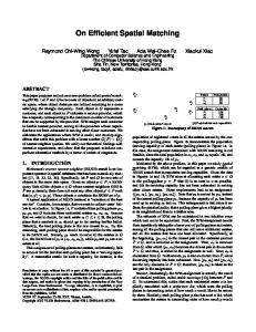
Figure 1 shows the SAMS dataflow. Data records in streams arrive continuously. They are matched against continuous queries registered in the system, and are stored in the database. Old stream data are truncated to keep the database manageable. Analysts selectively formulate the conditions of anomalies or potential hazards as continuous 3

queries, and register them with the SAMS. Registered queries are scheduled periodical executions over the data streams, and return new results (e.g. alerts), if any.

Figure 1: Data Flow of a Stream Anomaly Monitoring System

2.1

SAMS Characteristics

Formulating a query to capture anomalies or potential hazards buried in the data streams is a complex process. For many cases, an anomaly or hazard is too complex to be accurately represented as a query, and/or an accurate form is too expensive to evaluate. Therefore, an analyst usually formulates a continuous query that contains necessary but possibly not sufficient conditions of anomalies or hazards. The results of the continuous query invites the analyst’s further investigation the scope of which may be far beyond the capability of a declarative or procedural language. For example, the analyst may search text information in libraries or on Internet to understand correlations between a disease and patients’ geographies, or to know more about the relations between two organizations. To formulate a continuous query, the analyst may start with a set of identified anomalies and hazards in historical data. He may use clustering tools to inspect and analyze the data, and induce/hypothesize necessary conditions of anomalies or hazards. To ensure that the induced conditions return reasonable results, the analyst may formulate the conditions as an ad hoc query (an ad hoc query is a one-time query compiled and executed against a Database snapshot), and run it against the historical data. Based on the returned results, the analyst may refine or rehypothesize the conditions. Several trial and error runs may be needed to decide the proper set of the query conditions. Therefore, a SAMS should support fast ad hoc query executions, and easy or automated conversion from an ad hoc query to a continuous query is preferable to reduce the analyst’s query formulating effort. Satisfaction of a continuous SAMS query is often rare, even if the query only tests necessary conditions of anomalies or hazards. It is usual that a query returns no new results in days. This is because a query result represents a potential anomaly or hazard, and by its very nature is rare. Also, to reduce postprocessing work by human, an analyst refines the query to return as few false positive results as possible, namely formulates the query with the maximum necessary conditions to filter out as many uninteresting data as possible. This characteristic distinguishes SAMS from many other stream applications that work with sensor data, network traffic data, or Internet data. By appropriately arranging the operators of the query plan, it is very likely to make every set of intermediate results very small. Materialization of intermediate results is therefore a feasible approach to incremental evaluation

4

and computation sharing. Many stream projects developed extensions to SQL to support rich sets of window specifications, such as STREAM CQL [4] and TelegraphCQ’s for-loop constructs [14]. Comparing to these extensions, SAMS uses only time-based sliding windows, which can be naturally formulated as query predicates over data attributes. The purpose of introducing sliding windows is to convert the operations on unbounded streams to bounded data sets. For many stream applications, stream tuples are timestamped at the time they are generated, and the meaningful sliding windows are defined on the timestamp attribute. Due to various reasons, such as network delays and hardware failures, the arrival of the data tuples of an input stream may not restrictively conform to the timestamp order. Some stream systems relax the conformance to the data arrival order. The relaxation of the conformance is measured by a slackness parameter, which can be defined as a number n, or a fixed length of time T . When the slackness is defined as a number n, the system assumes that a tuple d generated at time τ will never arrive after more than n tuples that are later than τ arrive to the system. In other words, the system ignores a tuple d generated at time τ if the number of tuples later than τ that arrive before d exceeds the slackness parameter n. Slackness can also be defined as a fixed length of time T. After the system sees a tuple generated later than time τ + T , the system assumes that no tuple generated at time τ or earlier will arrive in the future. The slackness parameter T is used in SAMS to decide when to truncate old stream data without fearing that any future data tuples may join or aggregate with the discarded data. Data truncated from the stream will not participate in continuous query evaluation any more, but a substantial portion or its totality may remain in the database for historical data analysis. It is worth noticing that the SAMS slackness is different from other systems’ slackness notion, such as Aurora’s slackness. Aurora’s slackness is a query-level parameter that tells query executor what slack data to be ignored. SAMS slackness is a stream-level parameter. The value of SAMS slackness should conform to the stream characteristics. For example, assume a stock trading transaction is timestamped at its closing time and it must be reported to the system once it is closed, then setting the slackness T = 2 days may be sufficient for truncation purpose. In terms of query semantics, a SAMS must support selection, join and aggregation. Support of selection and join over aggregated values is also needed. We call selection and join over aggregated values post-aggregation. Postaggregation can be realized by defining views over aggregated values, and formulating the select-project-join query over the views. For some stream applications, such as network traffic analysis and sensor data applications, data aggregations are basic operations. In many cases, data items are first grouped and aggregated before filtering and joining. Post-aggregation is prevalent in such systems. This is due to the fact that data statistics are very important for decision making in those systems. The statistic feature of the data streams also justifies the employment of approximation techniques when the system is overloaded. However, this is not the case for SAMS streams. We summarize the SAMS characteristics as following: • A SAMS must support fast ad hoc query executions over a large volume of historical data. • Easy or automated conversion from an ad hoc query to a continuous query is preferable. • Matching results for continuous queries is not typically frequent. • A SAMS uses only application or user settable time-based sliding windows. • SAMS slackness is a stream-level parameter. • A SAMS does not require the output to be in strict time order. • A SAMS supports the following SQL query semantics: selection, join, aggregation, and post-aggregation. • Aggregation and post-aggregation are not prevalent in a SAMS. • Approximation techniques are not employed in a SAMS. • Continuous queries may number in the thousands or tens of thousands. • Daily stream volumes may exceed millions of records.

5

2.2

SAMS Query Examples

We choose the FedWire money transfer domain for illustration and experiments in this paper. For this particular application, there is a single data stream that contains money transfer transaction records, one record per transaction. A relevant subset of the attributes of the stream is shown below TRANID TYPE CODE TRAN DATE AMOUNT SBANK ABA SBANK NAME RBANK ABA RBANK NAME ORIG ACCOUNT BENEF ACCOUNT

NUMBER(10), NUMBER(4), DATE, NUMBER, NUMBER(9), VARCHAR2(100), NUMBER(9), VARCHAR2(100), VARCHAR2(50), VARCHAR2(50),

– – – – – – – – – –

transaction id, the primary key transfer type transaction date transfer amount sending bank ABA number sending bank name receiving bank ABA number receiving bank name originator account beneficiary account

We present several continuous query examples, and formulate the queries in SQL language. Post-aggregation is realized by defining views (subqueries are more expressive in terms of specifying correlated queries). Example 1 The analyst is interested if there exists a bank, which received an incoming transaction over 1,000,000 dollars and has performed an outgoing transaction over 500,000 dollars on the same day. The query can be formulated as: SELECT

FROM WHERE

r1.tranid rtranid, r2.tranid stranid, r1.rbank name rbank name, r1.tran date rtran date, r1.amount ramount, r2.amount smount transaction r1, transaction r2 r1.rbank aba = r2.sbank aba AN D to char(r1.tran date, 0 Y Y Y Y M M DD0 ) = to char(r2.tran date, 0 Y Y Y Y M M DD0 ) AN D r1.amount > 1000000 AN D r2.amount > 500000;

Example 2 For every big transaction, the analyst wants to check if the money stayed in the bank or left it within ten days. The query can be formulated as: SELECT r1.tranid rtranid, r2.tranid stranid, r1.rbank name rbank name, r1.benef account benef account, r1.tran date rtran date, r2.tran date stran date, r1.amount ramount, r2.amount smount FROM transaction r1, transaction r2 WHERE r1.rbank aba = r2.sbank aba r1.benef account = r2.orig account r1.tran date = r2.tran date r1.amount > 1000000 r2.amount = r1.amount;

AN D AN D AN D AN D AN D

Example 3 For every big transaction, the analyst again wants to check if the money stayed in the bank or left it within ten days. However he suspects that the receiver of the transaction would not send the whole sum further at 6

once, but would rather split it into several smaller transactions. The following query generates an alert whenever the receiver of a large transaction (over $1,000,000) transfers at least half of the money further within ten days of this transaction. The query can be formulated as: SELECT

FROM WHERE

GROUP BY HAVING

r.tranid tranid, r.rbank aba rbank aba, r.benef account benef account, AV G(r.amount) ramount, SU M (s.amount) samount transaction r, transaction s r.rbank aba = s.sbank aba r.benef account = s.orig account r.tran date AV G(r.amount) ∗ 0.5;

AN D AN D AN D AN D

Example 4 Suppose for every big transaction of type code 1000, the analyst wants to check if the money stayed in the bank or left within ten days. An additional sign of possible fraud is that transactions involve at least one intermediate bank. The query generates an alert whenever the receiver of a large transaction (over $1,000,000) transfers at least half of the money further within ten days of this transaction using an intermediate bank. The query can be formulated as: SELECT r1.sbank aba sbank, r1.orig account saccount, r1.rbank aba rbank, r1.benef account raccount, r1.amount ramount, r1.tran date rdate, r2.rbank aba ibank, r2.benef account iaccount, r2.amount iamount, r2.tran date idate, r3.rbank aba f rbank, r3.benef account f raccount, r3.amount f ramount, r3.tran date f rdate FROM transaction r1, transaction r2, transaction r3 WHERE r2.type code = 1000 r3.type code = 1000 r1.type code = 1000 r1.amount > 1000000 r1.rbank aba = r2.sbank aba r1.benef account = r2.orig account r2.amount > 0.5 ∗ r1.amount r1.tran date 1000000

AN D

Pattern 2: r2.type code

= 1000

r3.type code

= 1000

and Pattern 3: respectively. Other conditions are inter-tuple features, or join predicates. Particularly, following are the inter-tuple features that join the first two tuples: r1.rbank aba r1.benef account r2.amount r1.tran date r2.tran date

= = > ≤ ≤

r2.sbank aba AN D r2.orig account AN D 0.5 ∗ r1.amount AN D r2.tran date AN D r1.tran date + 10

= = = ≤ ≤

r3.sbank aba r3.orig account r3.amount r3.tran date r2.tran date + 10

and the following are that join the last two tuples: r2.rbank aba r2.benef account r2.amount r2.tran date r3.tran date

AN D AN D AN D AN D

Figure 3 shows a Rete network of the query. In this Rete network, data tuples that pass Pattern 1 and Pattern 2 are joined first, then the results are joined with data tuples that pass Pattern 3. Joining Pattern 2 and Pattern 3, then Pattern 1 is also logically correct. However, the different orders of joins could affect performance dramatically as observed with traditional query optimization techniques. Figure 4 shows the dataflow of a possible logical plan for the query which could be generated by a conventional DBMS query compiler. Figure 5 shows the dataflow of the Rete network. The logical plan and the Rete network have similar data access paths. However, in the Rete network, only necessary computations on the new data are carried out. The intermediate results are materialized in the database tables. Now we use a small data set shown in Table 1 to illustrate how the Rete network works as new data continuously arrive. Suppose that the data records (tuples) arrive in the order of the tranid. At Time 0, there are 2 records, and the Rete network is in the status shown in Figure 6. Note that if no new data satisfy at a certain node, then none of its succeeding nodes needs to be evaluated. In this case, no data satisfies the node joining Pattern 1 and Pattern 2, so its succeeding nodes does not need to be evaluated. At Time 1, two new records arrive. The Rete network is updated as in Figure 7. At Time 2, one more new record arrives, as shown in Figure 8, it triggers the generation of an alert. A continuous query may contain multiple SQL statements and a single SQL statement may contain unions of multiple SQL terms. Multiple SQL statements allow an analyst to define views. Each SQL term is mapped to a sub-Rete network. These sub-Rete networks are then connected to form the statement-level sub-networks. And the statement-level sub-networks are further connected based on the view references to form the final query-level Rete network. In summary, a Rete network performs incremental query evaluation over the delta part (new stream data) and materializes intermediate results. The incremental evaluation makes the execution much faster. However, there 11

Figure 3: A Rete Network for Example 4

! " #

" #

Figure 4: An Sample Logical Query Execution Plan for Example 4

is a potential problem when any materialized intermediate table is very large, which deteriorates the incremental evaluation performance severely. Only when the intermediate tables are fairly small, can the incremental evaluation scheme show consistent big advantages. Fortunately, since queries are not expected to be satisfied frequently, there

12

! " #

" #

Figure 5: The Data Flow of the Rete Network for Example 4 tran id 1 2 3 4 5

type code 1000 1000 1000 1000 1000

tran date 12/01/02 12/02/02 12/03/02 12/05/02 12/06/02

amount 400,000 1,200,000 305,000 800,000 800,000

sbank name PNC PNC Citibank Citibank Chase

rbank name Fleet Citibank Fleet Chase Citizen’s

orig account 1000001 3000001 3000001 2000001 4000001

benef account 1000009 2000001 2000009 4000001 5000009

Table 1: A Small Data Set to show how the Rete Network works are usually highly selective conditions that make the intermediate tables fairly small. We investigated several effective ways of reducing the sizes of the intermediate tables. We will also discuss the cases in which intermediate tables can not be reduced to small sizes.

4

ARGUS Profile System Design

As shown in Figure 2, the ARGUS Profile System contains two components. One is the database created on the Oracle DBMS, and the other is the Rete construction module, ReteGenerator. A profile is translated into a Rete network by ReteGenerator. Then the Rete network is registered in the database. The registration includes creating the intermediate tables, initializing the tables based the historical data, and storing and compiling the Rete network wrapped in the stored procedure. The database schedules periodical runs of the active Rete networks against new data.

4.1

Database Design

A simplified ARGUS database schema is shown in Figure 9. New data arrives continuously and is appended to the data table. Do queries() is a system level procedure that finds all the active queries from QueryTable in the order of their priorities, and executes them one by one. If any query is satisfied, an alert is generated. The job of running the procedure Do queries() is scheduled periodically. QueryTable records query information, one entry per query. Each 13

Figure 6: The Status of the Rete Network for Example 4 at Time 0. Records in the intermediate tables are represented by their tranids.

Figure 7: The Status of the Rete Network for Example 4 at Time 1. Records in the intermediate tables are represented by their tranids.

14

Figure 8: The Status of the Rete Network for Example 4 at Time 2. Records in the intermediate tables are represented by their tranids.

entry contains the query ID, the procedure name to call, the query priority, and a boolean flag indicating whether the query is active or not. Only active queries are executed in a scheduled run. The query priorities set the order in which the query procedures are called. For example, a procedure with priority 1 precedes a procedure with priority 10.

4.2

Restrictions on the SQL

To apply the Rete algorithm, we impose some restrictions to the SQL queries. Therefore, the set of queries that the Rete networks support is a subset of the standard SQL language. Nevertheless, the subset is rich enough for a SAMS. The first restriction is that the selection conditions of an SQL statement should be in a relaxed Disjunctive Normal Form. This means that the disjunctive selections should be specified by UNION unless the disjunctive predicates operate on a single table. For example, for the following SQL: SELECT r1.a FROM table1 r1, table2 r2 WHERE (r1.a < r2.b OR r1.a > r2.c) AN D (r1.d < 1 OR r1.e > 2); The Rete algorithm expects the input of the equivalent form:

15

!

"

#

Figure 9: ARGUS Database Design

SELECT r1.a FROM table1 r1, table2 r2 WHERE r1.a < r2.b AN D (r1.d < 1 OR r1.e > 2) UNION SELECT r1.a FROM table1 r1, table2 r2 WHERE r1.a > r2.c AN D (r1.d < 1 OR r1.e > 2); Note that the disjunctive form of (r1.d < 1 OR r1.e > 2) is allowed in an SQL because all the conditions in the form involve only one table. However, the other disjunctive form, (r1.a < r2.b OR r1.a > r2.c), is expected to be realized with UNION of two SQLs because the conditions in the form involve multiple tables. For the Rete algorithm, selection predicates on a single table, even with disjunctions, are easily evaluated in one step. However, disjunctive selection predicates over multiple tables are not easy. By pushing up disjunctions to the top level, we restrict each sub-Rete network in a conjunctive form, and results are unioned in the last step. The second restriction is that the current system doesn’t support multiple-way joins. It will reject an SQL statement with purely multiple-way joins, which is rare in real applications. For example, the following multiple-way join statement is not accepted by the ReteGenerator: SELECT r1.a FROM table1 r1, table2 r2, table3 r3 WHERE r1.a + r2.b = r3.c; But it accepts the following equivalent statement:

16

SELECT FROM WHERE

4.3

r1.a table1 r1, table2 r2, table3 r3 r1.e = r2.e AN D r2.f = r3.f AN D r1.a + r2.b = r3.c;

Translating SQL Queries into Rete Networks

A query formulated by an analyst is a set of SQL statements. The corresponding Rete network is a database stored procedure translated by ReteGenerator. Appendix A shows a sample translation of the query in Example 4 into a Rete network wrapped in an Oracle stored procedure. To simulate the topological connections of the Rete network, each node is associated with a Rete Flag, and maintains a list of Rete Flags of its children nodes (children flag list). A Rete Flag indicates whether the node needs to be updated or not. The default value of a Rete Flag is false. It is set to true only if any children flag is true which indicates that the update to the associated table is necessary. If none of children Rete Flags is true, then the node doesn’t need to be updated. To install a Rete network, we need both the procedure and a set of auxiliary DDL statements that create the intermediate tables and initialize the tables to contain the results on historical data. The initialization is necessary when the old data is present. Appendix B shows the corresponding DDL statements for the Rete network of Example 4. ReteGenerator contains three components: the SQL Parser, the Rete Topology Constructor, and the Rete Coder. The SQL Parser parses a set of SQLs to a set of parse trees, the Rete Topology Constructor rearranges the connections of nodes in a parse tree to obtain the desired Rete network topology, and the Rete Coder traverses the reconstructed tree, and generates the Rete network code in Oracle PL/SQL language. The SQL Parser takes the query (a set of SQLs) as input, and outputs a set of parse trees. Figure 10 shows the structure and the data flow of the parser. It contains an SQL parsing module and a lexer module. The SQL parsing module is a Perl package generated by a compiler compiler Perl-byacc [20] based on an SQL grammar [48]. The lexer module is also a Perl package [82]. The lexer is called by the SQL parsing module to tokenize the input query. The stream of tokens is fed to the SQL parsing module to generate the parse trees. The tools we used, namely, Perl-byacc, Perl Lexer, and the SQL grammar, were all from open sources, and were modified to meet our special needs. 4.3.1

Rete Topology Construction

Rete Topology Constructor constructs the network topology based on the selection predicates and join predicates. Only the where clause subtree decides the Rete Topology. Figure 11 shows the schematic subtree of the query in Example 4. Note that this subtree is pretty flat with all conditions on the same level, which is purposely done during parsing for easy reconstruction of the Rete network. Rete Topology Constructor, a Perl function, goes through the following three steps to construct the Rete topology. First, predicates are classified based on the tables they use. For the subtree in Figure 11, the classifications are shown in Figure 12. Second, the classified sets of the predicates are sorted based on the number of tables that the sets contain: [r1, r2, r3, (r1, r2), (r2, r3)] Each set corresponds to a node in the reconstructed subtree. From now on, we will use the term node to refer a classified set of predicates. Finally, the new subtree is reconstructed bottom-up. We first look for a pair of single-table nodes for the merge step. A pair of single-table nodes can be merged if there is a joint-table node joining just these two tables. Merge continues until all nodes are merged into a single node. Figure 13 shows the reconstructed subtree. 4.3.2

Aggregation and Union

An SQL statement may contain groupby/having clauses. If it also contains a where clause, the Rete network is generated for the where clause and the output of the Rete network is stored in a table, which will be the input to

17

Figure 10: Building the SQL Parser

! "

Figure 11: The where clause parse tree for Example 4

groupby/having clauses. We tried two methods for handling groupby/having clauses. The first method, implemented in our system, does the operations of grouping and having always on the whole input table, and finds the difference between the current results and the previous results. The difference is considered as the incremental results. The

18

r1 : r1.type code = 1000 r1.amount > 1000000 r2 : r2.type code = 1000 r3 : r3.type code = 1000 r1, r2 : r1.rbank aba = r2.sbank aba r1.benef account = r2.orig account r2.amount > 0.5 ∗ r1.amount r1.tran date