artificial neural networks in the forecasting of wave ... - CiteSeerX

ARTIFICIAL NEURAL NETWORKS IN THE FORECASTING OF WAVE PARAMETERS O. Makarynskyy

Post-Doctoral fellow at the Instituto Superior Técnico Lisbon, Portugal

A.A. Pires-Silva

D. Makarynska

Instituto Superior Técnico Doctoral student at the Lisbon, Portugal Instituto Superior Técnico Lisbon, Portugal

C. Ventura-Soares

Instituto Hidrográfico Lisbon, Portugal

1. INTRODUCTION The predictions of wind wave characteristics with different lead times are necessary in a large number of coastal and open ocean activities. Numerical wave models, which usually provide this information, are based on deterministic equations and in some cases they do not entirely account for the complexity and uncertainty of the wave generation and dissipation processes. Assessing the present status of the spectral wind wave modeling, Liu et al. (2002) compared four prediction models representing different levels of sophistication all based on the concept of a wave energy spectrum. It was concluded that the models performed in a similar way reflecting the general trend and patterns presented in observations. The differences between the results of computations were of the same order of magnitude as the differences between model results and observations. There is, therefore, a certain need to explore alternative approaches. This paper reports the development and testing of a methodology based on the artificial neural network concept to predict wave parameters, namely, the significant wave height, the zero- up-crossing wave period and the peak wave period. In recent years, artificial neural networks have been used in a number of coastal engineering applications due to their ability to approximate the nonlinear mathematical behavior without a priori knowledge of interrelations among the elements within a system. The applications range from assessing the stability of rubble-mound breakwaters (Mase et al., 1995), studying the storm-built beach profile predictability (Tsai et al., 2000), to the forecast of the tide level (Tsai and Lee, 1999), sea level (Roske, 1997), sea currents (Babovic, 1999), daily river stage (Thirumalaiah and Deo, 1998 and 2000), salinity variations in a tidal environment (Huang and Foo, 2002) and wave heights (Deo et al., 2001; Agrawal and Deo, 2002). The paper is structured as follows. A general outline of neural nets is presented in Section 2. The data used to train and validate neural networks described in Section 3. Several sets of neural networks simulations with different numbers of neurons in the input and hidden layers are presented in Section 4. This includes a comparison of values estimated from measurements versus predicted ones in terms of root mean square error, correlation coefficient and scatter index as well as some results of saliency analysis implementation. Section 5 gives some final remarks.

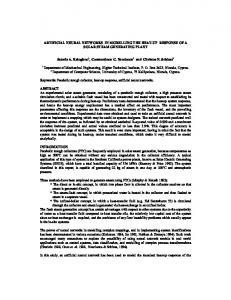
2. ARTIFICIAL NEURAL NETWORKS The inspiration for the development of artificial neural networks, that started about 60 years ago, was found in the biological neural system. However, the artificial nets are still very primitive comparatively to the biological ones (Fausett, 1994). Neural networks belong to that type of information-processing systems, which allow an approximation to the nonlinear behavior (Haykin, 1999) that is characteristic in geophysical processes. The basis of a neural net is the concept of neuron considered as a unit (Fig.1). The unit takes an argument (n), which can be formed as a sum of a weighted input (pw) and a bias (b), and by means of a transfer (activation)

function (f), typically a step function or a sigmoid function, produces an output (a). Note that there can be many input-weight pairs (piw i,j , i=1,…,N – number of input nodes, j=1,…,R – number of neurons in the first hidden layer) to form a unique argument (nj ) of the transfer function in a jth neuron. Several such neurons can be combined in a layer, whereas a particular network can contain one or more interconnected layers of neurons.

p

w

S

n

ƒ

a

b Input

Neuron

Fig.1. A neuron with a single scalar input and a bias The method of determining weights and biases is called learning. The learning process requires a set of patterns “input – target output” of proper network behavior. During the learning process the weights and the biases of the network are iteratively adjusted to minimize the error between the network outputs and the target outputs urging the entire network to perform in some expected way.

3. DATA EMPLOYED The data from a “WAVEC” buoy, which is moored in 97 m depth offshore of Sines Harbour (S ines 1D buoy, 37o 55’ 16” N, 8o 55’ 44” W) (Fig.2) and is explored operationally by the Hydrographic Institute of the Portuguese Navy, were used to train and test the neural networks. The estimated values of Hs, T02 and Tp for the period December 4, 1999, 00 a.m. - January 31, 2000, 21 p.m., at the synoptic times (each three hours starting from 0000 GMT), were divided into two data sets. Data set 1 of each of these wave parameters was used for learning of the corresponding neural networks, while data set 2 served for validation purposes. The common three- layer feed-forward networks, with a non- linear differentiable log- sigmoid transfer function in the hidden layer (consisting of several nodes) and line ar transfer function in the output layer (consisting of one node in all the cases), were used in this study.

Fig.2. Location of the Sines 1D buoy station (star) at the Portuguese coast

The natural processes, which define the variability of the wave parameters in time domain, are different. Therefore, a separate network was invo lved to simulate each wave parameter with each leading time. This also allowed keeping relatively simple the architectures (patterns of interconnections between layers of neurons) of networks. The resilient backpropagation training algorithm was implemented to train the nets. This algorithm is generally much faster than the generally used steepest descent algorithm. The number of training epochs in each simulation was 1000.

4. FORECASTING OF WAVE CHARCTERISTICS It was initially assumed that a 24 hours history (eight measurements) contains all the necessary information to simulate the wave characteristics one (+3 hours), two (+6 hours), four (+12 hours) and eight (+24 hours) steps ahead. Thus, at the beginning each input layer of the separate neural networks developed to predict Hs, T02 and

Tp consisted of 8 nodes, while each output layer had one node. The number of nodes in the hidden layer (h) of these nets was computed according to the expression used by Huang and Foo, (2002) h = (2n + 1),

(1)

where n is the number of input nodes. The performance of the artificial neural networks involved into forecasting was estimated in terms of root mean square error (RMSE), correlation coefficient (R) and scatter index (SI), computed as N

∑( y

− xi ) 2

i =1

RMSE=

N

N

∑ (x R=

i

i

,

− x )( y i − y )

i =1

N

∑(x i =1

N

i

(2)

.

(3)

− x ) 2 ∑ ( yi − y) 2

SI=

i =1

RMSE , x

(4)

where x i is an observed value at the i-th time step, yi is a simulated value at the same moment of time, N is the number of time steps, x is the mean value of observations, and y is the mean value of simulations. The results of simulations obtained using the networks architecture 8 x 17 x 1 (numbers of nodes in the input x hidden x output layers) are presented in Table 1. The verification statistics show that values of Hs were simulated very well when short prediction intervals of three and six hours are concerned. The RMSE are less or equal to 0.20 m, coefficients of correlation are higher than or equal to 0.94 and scatter indexes of these forecasts are less than or equal to 0.18. The predictions of Hs for 12 hours were less bright but even so they are comparable to the same set of verification statistics presented in (Carretero et al., 2000). The predictions with leading time of 24 hours exhibit neither a reliable correlation pattern nor reasonable values of RMSE and SI. Table 1. Verification statistics of H s, T02 and Tp simulations with different lead times. Numbers of nodes in the input x hidden x output layers are 8 x 17 x 1. Here RMSE is the root mean square error, R is the correlation coefficient, SI is the scatter index. Hs T02 Tp RMSE(m) R SI RMSE(s) R SI RMSE(s) R SI +3 0.14 0.97 0.12 0.88 0.89 0.14 1.75 0.63 0.14 +6 0.20 0.94 0.18 1.13 0.81 0.18 1.89 0.49 0.15 +12 0.37 0.82 0.32 1.56 0.64 0.24 2.13 0.35 0.17 +24 0.77 0.40 0.66 1.93 0.41 0.30 2.26 0.14 0.17 To illustrate these considerations, in Fig.3 and 4 time series plots and scatter diagrams of the significant wave heights estimated from observations and simulated with different lead times are displayed. The mean wave period was simulated reasonably well for three and six hours period of forecasting. The root mean square errors are around 1 s, the coefficients of correlation are higher than or equal to 0.81 and the scatter indexes are less than or equal to 0.18. The predictions for 12 and 24 hours were less successful showing low correlation coefficients although with fairly good values of RMSE and scatter index.

Fig. 3. Significant wave heights obtained from Sines 1D buoy and simulated by neural nets with architecture 8x17x1 for different leading times for the period January 12 – 31, 2000.

Fig. 4. Scatterplots of the significant wave heights simulated by neural nets with architecture 8x17x1 for different leading times versus obtained from Sines 1D buoy. The peak wave period was the most difficult value to forecast. The predictions with one step ahead show a relatively low value of the correlation coefficient (0.63), which still decreases in forecasts for larger time scales. Nevertheless, the other verification statistics are reasonably good: the values of the root mean square error are about 2 s and of the scatter indexes are less than or equal to 0.17. Agrawal and Deo (2002) reported a higher (in terms of correlation coefficient) performance of the network with only two input nodes (the current and preceding values) used to predict the significant wave height one step ahead. Their study was based on the data from Yanam, a site at the eastern side of the Indian coastline in 88 m depth. Saliency analysis is a technique that allows to estimate the relative importance of the input and/or the processing components of a network by intentional introduction of missing units (Abrahart et al., 2001). This technique was derived from the idea that a neural network, which is a parallel distributed processing system, should operate sufficiently well even in the case of incomplete input or when one of its internal components faults. Note that this technique is not a form of sensitivity analysis because individual items are not exposed to any change but removed completely. Tables 2 and 3 demonstrate an application of saliency analysis to simulations of Hs, T02 and Tp. The technique was used to assess the role of the units in both the input and hidden layers. The values displayed in Table 2 show that the use of twice less nodes in the input layer (12 hours history) and corresponding to the expression (1)

number of neurons in the hidden layer, not only does not degrade the forecasts significantly but improves the statistics considered. Table 2. Verification statistics of Hs, T 02 and T p simulations with different lead times. Numbers of nodes in input x hidden x output layers are 4 x 9 x 1. Here RMSE is the root mean square error, R is the correlation coefficient, SI is the scatter index. Hs T02 Tp RMSE(m) R SI RMSE(s) R SI RMSE(s) R SI +3 0.15 0.97 0.13 0.83 0.91 0.13 1.72 0.64 0.13 +6 0.21 0.94 0.18 1.11 0.83 0.17 1.88 0.51 0.15 +12 0.31 0.89 0.26 1.45 0.70 0.22 2.08 0.37 0.16 +24 0.53 0.74 0.45 1.71 0.55 0.26 2.16 0.20 0.17 Table 3. Verification statistics of Hs, T 02 and T p simulations with different lead times. Numbers of nodes in input x hidden x output layers are 2 x 5 x 1. Here RMSE is the root mean square error, R is the correlation coefficient, SI is the scatter index. Hs T02 Tp RMSE(m) R SI RMSE(s) R SI RMSE(s) R SI +3 0.15 0.97 0.13 0.82 0.91 0.13 1.69 0.65 0.13 +6 0.21 0.94 0.17 1.11 0.83 0.17 1.94 0.47 0.15 +12 0.34 0.84 0.27 1.39 0.72 0.21 2.05 0.37 0.16 +24 0.53 0.69 0.45 1.69 0.54 0.26 2.16 0.16 0.17 However, the further simplification of the networks architecture (Table 3) produces a mixed effect: some statistics slightly improve (for instance, the predictions of T02 for six hours and Tp for three hours), while others degrade (simulations of Hs with leading time of 12 and 24 hours). The time series plots and scatter diagrams of the zero-up-crossing wave periods, estimated from measurements and simulated using artificial neural networks with three different architectures (8x17x1, 4x9x1 and 2x5x1) and presented in Figures 5 – 9, illustrate the effects of the modeifications.

Fig.5. Zero-up-crossing wave periods obtained from Sines 1D buoy and simulated by neural net with architecture 8x17x1 for 24 hours lead time for the period January 12 –31, 2000. Thus, the implementation of saliency analysis revealed that the performance of the artificial neural networks employed in forecasting of Hs , T02 and Tp with leading times of 3, 6, 12 and 24 hours can be, to some extent, improved with simplification of the initial networks architecture. Besides, the reduction of the number of neurons in both the input and hidden layers allows a faster training of the networks.

Fig.6. Zero-up-crossing wave periods obtained from Sines 1D buoy and simulated by neural net with architecture 4x9x1 for 24 hours lead time for the period January 12 –31, 2000.

Fig.7. Zero-up-crossing wave periods obtained from Sines 1D buoy and simulated by neural net with architecture 2x5x1 for 24 hours lead time for the period January 12 –31, 2000.

Fig. 8. Scatterplots of the zero- up-crossing wave periods simulated by neural nets with architectures 8x17x1 and 4x9x1 for 24 hours lead time versus obtained from Sines 1D buoy.

Fig. 9. Scatterplots of the zero-up-crossing wave periods simulated by neural net with architecture 2x5x1 for 24 hours lead time versus obtained from Sines 1D buoy.

5. CONCLUDING REMARKS Artificial neural networks were used to predict significant wave heights, zero- up-crossing wave periods and peak wave period with leading times of 3, 6, 12 and 24 hours. The simulations were compared to time series of these wave parameters estimated offshore the west coast of Portugal. The results show different levels of performance of each of the neural networks in terms of the root mean square error, correlation coefficient and scatter index. The behavior changed according to the parameter being predicted and the period of forecasting. The nets simulating integral wave parameters (Hs and T02 ) and short lead times (three and six hours) performed generally better than the ones developed for longer periods and to predict the peak wave period. An implementation of the saliency analysis technique allowed estimating the relative importance of the input units and the processing units of the neural networks employed in simulations and, in this case, simplifying the networks architecture. The simplifications introduced increased the accuracy of the simulations. Fairly good predictions of the significant wave height were produced for all the lead times. The forecasts of zero-up-crossing wave periods for 3, 6 and 12 hours were also improved. The simulations of the peak wave period showed no reliable correlation pattern in the sets of the data engaged in the forecasts. This issue should be further addressed employing other architectures of neural networks and/or using data assimilation techniques.

ACKNOWLEDGMENTS The Hydrographic Institute of the Portuguese Navy is gratefully acknowledged for making available the buoy data. Oleg Makarynskyy acknowledges a post-doctoral fellowship (SFRH/BPD/1507/2000) and Dina Makarynska acknowledges a doctoral fellowship (SFRH/BD/841/2000), both from “Fundação para a Ciência e Tecnologia” of the Ministry of Science and Technology of Portugal. This work is part of the research project “Nearshore Wind Wave Prediction: Data Assimilation and Spectral Models” (PDCTM/MAR/15242/99) funded by “Fundação para a Ciência e Tecnologia” of the Ministry of Science and Technology of Portugal.

REFERENCES Abrahart, R.J., See, L. and P.E. Kneal, 2001: Investigating the role of saliency analysis with neural network rainfall-runoff model. Computers & Geosciences, 27, 921-928. Agrawal, J.D. and M.C. Deo, 2002: On-line wave prediction. Marine Structures , 15, 57-74. Babovic, V., 1999: Subsymbolic process description and forecasting using neural networks. Proc. of the Int.Workshop: Numerical Modelling of Hydrodynamic Systems, (eds. P. Garcia-Navarro and E. Playan), 57-79. Carretero, J. C., Alvarez, E., Gomez, M., Perez, B. and I. Rodríguez, 2000: Ocean forecasting in narrow shelf seas: application to the Spanish coasts. Coastal Engineering, 41, 269–293. Deo, M.C., Jha, A., Chaphekar, A.S. and K. Ravikant, 2001: Neural networks for wave forecasting. Ocean Engng., 28, 889-898. Fausett, L., 1994: Fundamentals of neural networks. Architectures, algorithms, and applications , Prentice-Hall, 462pp. Haykin, S., 1999: Neural networks: a comprehensive foundation . Prentice-Hall, 842pp. Huang, W., and S. Foo, 2002: Neural network modelling of salinity variation in Apalachicola River. Water Research, 36, 356-362. Liu, P.C., Schwab, D.J. and R.E. Jensen, 2002: Has wind-wave modelling reached its limit? Ocean Engng., 29, 81-98. Mase, H., Sakamoto, M. and T. Sakai, 1995: Neural network for stability analysis of rubble-mound breakwaters. J. Waterway, Port, Coastal and Ocean Engng., ASCE, 121 (6), 294-299. Roske, F., 1997: Sea level forecasts using neural networks. German J. of Hydrography, 49 (1), 71-99. Thirumalaiah, K., and M.C. Deo, 1998: River stage forecasting using artificial neural networks. J.Hydrologic Engng., ASCE, 3 (1), 26-32. Thirumalaiah, K., and M.C. Deo, 2000: Hydrological forecasting using neural networks. J.Hydrol ogic Engng., ASCE, 5 (2), 180-189. Tsai, C.P., and T.L. Lee, 1999: Back-propagation neural network in tidal-level forecasting. J. Waterway, Port, Coastal and Ocean Engng., ASCE, 125 (4), 195-202. Tsai, C.P., Hsu, J.R.-C., and Pan, K.L, 2000: Prediction of storm-built beach profile parameters using neural network, Proc.27th Int. Conf. Coastal Engineering, ASCE, V.4, 3048-3061.