Assignment techniques on Virtual Networks Performance considerations on large multi-modal networks NECTAR conference Umeå, June 12-15 2003 Bart JOURQUINI, II and Sabine LIMBOURGI II
Facultés Universitaires Catholiques de Mons (FUCaM), Group Transport & Mobility (GTM) 151 Ch. de Binche, B-7000, Mons, Belgium Tel : 32-65-323211, Fax : 32-65-315691,
[email protected] II Limburgs Universitair Centrum (LUC) Universitaire Campus, gebouw D, B-3590 Diepenbeek, Belgium Tel : 32-11-268600, Fax : 32-11-268700
ABSTRACT Multi-Modal freight models are traditionally built following the well known “fours steps model” in which generation, distribution, modal-split and assignment are seen as separated modules. An alternative approach, implemented in some softwares, is to represent the multi-modal network by means of a mono-modal one, representing each particular transport operation (loading or unloading operation, transhipments, ...) by a dedicated “virtual link”. This approach is proven to give interesting results, but as the drawback to generate much larger networks as their geographic representation. These huge networks (often larger than several hundreds of thousands links) made it difficult to implement loop-based equilibrium assignment techniques. The increasing computation power of recent hardware make it now much more easy to test several alternative assignment techniques. This paper presents some results obtained on a large multi-modal network, using different equilibrium assignment algorithms.
-1-
1
Introduction
Until a few years ago, transport models were essentially focused on passengers flows. More recently, some freight specific network models have been developed but, like passengers models, they are essentially analysing networks from a "link" point of view rather than from a "node" point of view. Even if some of them deals to some extend with the different operations performed at the nodes, i.e. loading /unloading, transhipment or simple transit, their output still targets mainly transport flows on the networks. As a result of a trend towards economic globalisation, just in time deliveries and road transports expansion, a great deal of attention is paid nowadays to reorganisation of networks, intermodal transports and new technical bundling concepts in order to substitute to direct road transport alternative transport solutions with less negative external effects. Thus, there is a need for a better modelling of the functions assumed by nodes, i.e. terminals and transhipment platforms. Beyond this brief introduction, this paper will present an overview of the Virtual Network methodology implemented in the Nodus software developed at FUCaM-GTM. It will then discuss the most used assignment techniques and how they can be applied to Virtual networks. Finally, the performances of these methods will be discussed on small and large networks.
2
NODUS and Virtual networks
A geographical multimodal transport network is made of links like roads, railways or waterways, on which vehicles moves; at its nodes it is made also of connecting infrastructures these links like terminals or logistics platforms where goods are loaded, unloaded, transhipped or processed in different ways. To analyse transport operations over the network, costs or weights must be attached to these geographical links over which goods are transported and to the connecting points where goods are handled. However, most of these infrastructures can be used in different ways and with different costs. For example, boats of different sizes and operating costs can use the same waterway; at a terminal a truck's load can be transhipped on a train, bundled with some others on a boat or simply unloaded as it reached its destination. Normally, the costs of these alternative operations should be different.
-2-
2.1
The Building of a Virtual Network: an Intuitive Approach
A simple geographic network does not provide an adequate basis for detailed analyses of transports operations where the same infrastructure is used in different ways. To solve this problem, the basic idea, initially proposed by Harker (1987) and Crainic et al. (1990), is to create a virtual link with specific cost for a particular use of an infrastructure. The NODUS software proposes a methodology and an algorithm which creates in a systematic and automatic way a complete "virtual network" with all the virtual links corresponding to the different operations which are feasible on every real link or node of a geographic network. The software and its underlying methodology are discussed in Jourquin (1995) and Jourquin & Beuthe (1996). This permits to apply the methodology to extensive multimodal netwoks. The solution can be presented first in an intuitive way by using the example of a simple waterways network, as shown in Figure 1. This network consists of 4 nodes and 5 links. The “W” links represent waterways and the “R” links rail tracks. The numbers after these letters correspond to the transportation means that can be used on the links. So, “W1” represents a waterway that can support small barges and “W2” a waterway that can be used by both small and large barges. To go from node “a” to “d”, it could be possible that the route 1+3, using large barges and trains, is less expensive than the route 5, using exclusively small barges. It appears that computing costs and routes on this kind of networks is not immediate: •
different costs can be assigned on a single link, depending on which transportation means is used. In this example, the use of a small barge on link “W1” has a different cost than the use of a large barge on the same link;
•
the same is true for the nodes: in the given example, the simple transit of a small barge come from link 1 and going on link 2 can be done at no cost, but the transhipment from a large barge coming from link 1 onto a train that will go on link 3 represents an important cost.
This problem can be usefully handled on the corresponding virtual network illustrated in Figure 1, provided that the relevant costs are attached to each of the virtual links. As can be seen, the solution involves the creation of a set of virtual nodes and a set of virtual links connecting these nodes. Each real link has been split in as many virtual links as
-3-
there are possible uses; their end-nodes are connected by new virtual links corresponding to simple transit or transhipment operations at the real nodes. In this way, this network with multiple means use is represented by a unique but more complex network on which each link corresponds to a unique operation with a specific cost. Then, one cheapest path can be computed by means of an algorithm such as the one proposed by Dijkstra (1959) for low density graphs. The resulting solution is an exact solution, taking all the possible choices into account. We can now demonstrate how the virtual network is built on the basis of a rather simple, though somewhat complex notation, which provides a convenient way to link cost functions to virtual links. Table 1 enumerates the elements of the real network. Figure 1: Multimodal network
a
1 (W2)
b
2 (W1)
3 (R1)
5 (W1)
c
4 (R1)
(W1)
d In a first step, the virtual links corresponding to the real links, i.e. rail tracks, etc., must be generated. These are defined in Table 2 by their end-nodes, the notation of which indicates successively the node, the real link, the mode and the means. Table 1: Real network Link 1 2 3 4 5
Node 1 A B B D A
Node 2 B C D C D
Table 2: Travelling links
Type of link W2 W1 R1 R1 W1
-4-
Real links 1 2 3 4 5
End-nodes of virtual links a1W1 b1W1 a1W2 b1W2 b2W1 c2W1 b3R1 d3R1 d4R1 c4R1 a5W1 d5W1
Table 3: Connecting virtual links to node b Real node End-nodes of virtual links b b1W1 b2W1 b1W2 b2W1 b1W1 b3R1 b1W2 b3R1 b2W1 b3R1
Figure 2: Partial virtual network a1W1
b1W1
b2W1
c2W1
1 a5W1
c4R1 a1W2
b1W2 b3R1
d3R1
d5W1
d4R1
In a second step, these virtual links must be connected by transit or transhipment virtual links. To keep things as simple as possible, we just enumerate in Table 3 the connecting virtual links related to node “b”. They can be viewed in Figure 2, where the virtual network resulting from that procedure is presented when it is applied to all the nodes. In this network, the boldfaced links represent the links of the real network, possibly split up. The dotted links represent the transit virtual links, while the transhipment links are indicated by a thin continuous line. This network is not yet complete because it does not contain entry and exit nodes in/from the network. This can be done by the creation of additional virtual nodes associated to loading and unloading operations at nodes where they are possible. Those entry or exit points in the virtual network are referenced by adding “000” to the real node number. They must also be connected to other nodes by appropriate virtual links. In general, the weight given on a link can very well vary with the direction it is used; loading and unloading operations for instance don’t have necessarily the same cost, and
-5-
the cost of going upstream on a river is normally higher than going downstream. To solve that problem, all virtual nodes are doubled at generation time by adding a + or a – sign to their code; by the same token, all links are split into two oriented arrows connecting these new nodes. This is illustrated for real node b in figure 3. The virtual network requires the development of four types of cost functions, which are associated with specific virtual links through their notation: •
The use of a travelling cost function is indicated by a difference between the virtual link's indices denoting the real end-nodes;
•
Transit costs are applied when the link's indices denoting the two connected real links vary, whereas the mode and means indices remain the same;
•
For transhipment costs, the link's indices of the connected real links should vary, as well as the mode and/or means indices;
•
For loading/unloading costs, one of the two indices of the real links is "00000".
Those “doubled” virtual nodes also make it possible to avoid “unwanted movements”, like an unloading followed by a loading to circumvent a forbidden transhipment operation. Figure 3: Detailed virtual network at node
-
b1W1
b1W2
b000
+
+
-
-
+
+ +
-
b3R1
-6-
b2W1
Obviously, the codification used in the preceding figures is not suitable for real applications; using a single letter as node label would limit the size of the real network to 26 nodes! That’s why the virtual nodes are coded in the following way: a plus or minus sign, 5 digits for the node number, 5 digits for the link number, 2 digits for the mode and 2 digits for the means. Each label is thus represented by a 14 digits number preceded by a sign. 2.2
Cost Functions on Virtual Networks
After this overview of the basic methodology, it is necessary to explain how the cost functions are connected with the virtual network and which are their characteristics. As usual in transportation analysis (see, for example, Kresge and Roberts (1971), or Wilson and Bennet (1985)), "generalised cost", which allows to integrate all factors relevant for transport decision making in terms of monetary units, are used. The concept can be defined in different ways according to whether it is the point of view of the shipper which is taken or the one of the carrier, and according to the unit of reference which is used, i.e. tons, tons-km, vehicles, distances, etc. The specific cost functions which compose the generalised cost, obviously, must be coherent across modes and means, but their functional forms can be freely chosen. The virtual network requires the development of four types of cost functions, which are associated with specific virtual links through their notation: •
The use of a travelling cost function is indicated by a difference between the virtual link's indices denoting the real end-nodes;
•
Transit costs are applied when the link's indices denoting the two connected real links vary, whereas the mode and means indices remain the same;
•
For transhipment costs, the link's indices of the connected real links should vary, as well as the mode and/or means indices;
•
For loading/unloading costs, one of the two indices of the real links is "00000".
These four types of function are made of the following elements: •
All the costs related to moving a vehicle between a trip's origin and destination, like labour, fuel, insurance, maintenance costs, or tariffs;
•
The cost of inventory of the goods during transportation;
•
Handling and storage costs or tariffs, including packaging, loading and unloading and services directly linked to a transport.
-7-
All residual indirect costs like general administrative services which may be assigned to transports on an average basis. 2.3
Computing shortest paths on networks
The contemporary transport systems are used in an intensive way and are often congested at various degrees, particularly in urban areas. Transport models have to determine how the traffic is distributed over the transport network of which the structure and the capacity are known. This is the assignment problem. Unless no capacity constraints are taken into account (All-Or Nothing assignment), an assignment consists in the distribution of the traffic on a network considering the demand as well as the flows supported by the network (capacity). The assignment methods try to model the traffic’s distribution over a network taking into account a set of constraints, such as capacity and transport costs, in order to obtain an equilibrium. This type of problems can be solved by means of optimisation methods. We are interested here in the methods intended to model flows of commodities on large multimodal networks, using virtual network, which, as explained earlier, make it possible to combine modal choice and assignment in a single step. The results of the assignment, which depend on the sophistication of the implemented method, include an estimate of flows, travel duration and/or corresponding costs, for each link of the network. All the equilibrium assignment methods are based on the “all-or-nothing” algorithm. The principle of this algorithm is to compute the minimum weight path between each pair of origin and destination, and to allocate the total demand to be transported between these nodes onto this single path. As shown in Table 4, the Dijkstra’s algorithm, with a binary heap implementation, seems to be the best algorithm to be used on virtual networks (which is a graph with low density, as the number of links is far below the square of the number of nodes). The Dijkstra’s algorithm solves the problem of the shortest path from an origin to all the possible destinations. The algorithm of Johnson finds all the shortest paths between all the pairs of nodes of the graph, it using the algorithm of Bellman-Ford and Dijkstra. If we take the detailed virtual network generated from the Belgian network, we have approximately 300000 virtual links (M) and 100000 virtual nodes (N), of which 1500
-8-
(X) are potential (un)loading nodes. The latest characteristic involves that the Dijkstra’s algorithm is the most suitable, because only a small amount of nodes are relevant to compute paths from, because they are potential origins. Table 4: Complexity of shortest-path algorithms Linear (worst case)
Used priority queue Binary heap Fibonacci heap (worst case) (amortized analyze1)
Dijkstra’s algorithm O(XN²) O(XM log2N) O(XN log2N+XM) Executed X times Johnson’s algorithm O(N³) O(NM log2N) O(N² log2N+NM) Given N : number of nodes M : number of links X : number of nodes that are a potential origin or destination 1 A amortised analysis guarantees an average performance for each operation in the worst case.
Among the various implementations of this algorithm, the binary heap implementation gives the best results, because our graph is not dense (M is much lower than N²). The Fibonacci heap implementation gives smaller execution times only in the most unfavourable cases (15% of the cases tested on our networks) and is, on average, 50% slower than the binary heaps for our problems. We have also introduced a stop criterion in the Dijkstra’s algorithm. It stops indeed, as soon as the algorithm determined the shortest path to all the destinations to reach starting from a given origin. This improves the computing time by more than 50%, because the flows starting from a node are, in most cases, sent to only a few destinations that are relatively close to the origin. 2.4
Cost functions and congested links
The All-Or-Nothing (AON) algorithm presents however some limits because the flow of transport between two given nodes should be distributed between various alternate routes. The multi-flow algorithms make it possible to calculate those paths, but they don’t take into account any constraint. However, certain axes of the network suffer from congestion and this congestion also lead in the search of alternate routes, in order to balance the traffic on the network. The equilibrium algorithms try to model this phenomenon in transport systems. These models, which take into account the variation of the transportation generalized costs according to the assigned flows, consider that the distribution of the traffic on the network is the result of an interaction between the supply and the demand of transport.
-9-
They try to approach the equilibrium conditions stated formally by Wardrop in 1952. The second principle (or the design principle) states that: Under equilibrium conditions traffic should be arranged in congested networks in such a way that the average (or the total) travel cost is minimised. It is important to note that the fact of using these methods on a virtual network makes it possible to observe transfers of flow between the various transportation modes. Indeed, in opposition to the classical four stages models (generation, distribution, modal-split and assignment), and as specified higher, the virtual network combines the modal split and the assignment in a single step. Thus, an alternative route can very well be used, totally or partially, by another mode and/or means of transport. This is probably the principal contribution of the use of equilibrium assignment methods on virtual networks and will be illustrated in the next section. The traffic assignment models which take the effects of the congestion into account require a relation between the cost and flow on the network, which can be described in a general way like : Ca=Ca({V}). The cost on link “a” should be a function of flow V on the network and not only on the link itself. This is simplified by considering that Ca=Ca(Va) i.e. that the cost on link “a” is a function of the flow Va on it. A good cost function must have the following properties: it must be realistic, non decreasing, monotonous, continue, differentiable and should not generate infinite costs if the flow is equal or higher than the capacity. Many functions (Ortúzar and Willumsen (1990)) were proposed to describe this relation. The most used are : •
Smock (1962) : C = C 0 e
V /K
where C : cost for a given flow V C0 : cost at free flow K : capacity of the link β (V / K )
•
Overgaard (1967) generalises the previous function :
•
The Bureau of Public Roads (1964), USA, proposes the standard function which
(
is certainly the most used: C = C0 1 + α (V / K )β
C = C0 α
)
We used this latest function with α= 0.15 and β= 4, which are the most used values for the European networks.
- 10 -
2.5
Flow equilibrium algorithms
Various assignment algorithms which try to obtain a distribution of flows on the network approaching the equilibrium conditions stated by Wardrop can be found in the literature. The implementation of these algorithms on a virtual network is not immediate. Indeed, in the reality, congestion is observed on real links, not on virtual links. However, in a virtual network, the same real link is represented by various virtual links, according to the number of transportation means that are defined. It is thus necessary to consolidate the flows obtained on the virtual links before obtaining flows indeed assigned on the real links. A first technique, based on the method of the successive averages (MSA) was implemented in Nodus. During the initialisation step, for each link a, the flow Va is set to null and its associated cost C a is computed for a free flow situation. The process then enters in a loop that is repeated until a stop condition is satisfied. At a given iteration n, and for each link a, the cost C an is computed, that depends on the flow Van −1 found on the link at iteration n-1. A set of auxiliary flows Fan is then obtained by means of an AON assignment based on the just re-computed costs. The new flow Van is then obtained :
Van = (1 − λn )Van −1 + λn Fan , where λn =
1 n
The algorithm of Frank-Wolfe (FW) (1956) is very similar to the previous one. It differs from it only by the way λ is computed : instead of being fixed at 1/n, as it was the case in the method of the successive averages, it is calculated to optimise the displacement in the descent direction Fn–Vn-1. After each iteration, one have to compute the depth of the descent: Va
λn ⇐ min ∑ ∫ C a (V )dV a
0
where 0 ≤ λn ≤ 1 The effects of the congestion can also be taken into account by an incremental assignment (INC). At each iteration, only a restricted proportion of the demand matrix is assigned on the network. The incremental method charges the network gradually. The
- 11 -
total quantity to transport is split by a factor pi, such as
∑p
i
= 1 and, during each it-
i
eration, an additional increment is loaded on the network. We calculated these factors as follows: If n represents the number of iterations, then, pi =
n − i +1 where i=1,2, …,n n * (n + 1) / 2
The p’si are thus a decreasing arithmetic progression in which the difference between two successive terms is
−1 n * (n + 1) / 2
The main disadvantage of the incremental method is that once that a flow is assigned on a link, it is not more possible to withdraw a part of it in order to assign it to another link. This will be illustrated in the next section. The incremental method can also be associated the algorithm of Frank-Wolfe: to accelerate the convergence of the algorithm of Frank-Wolfe, the incremental method is used to obtain the initial flows (Inc+FW). When should the iterations be stopped? Except with regard to the incremental method, for which the number of iterations must be fixed a priori, we use the stop-rule of Le Blanc et al (1975) : Stop if max
(| Va( n ) − Va( n −1) |)