Asymptotic behavior of pre-test procedures

Asymptotic behavior of pre-test procedures

Pieta Boon Faculty of Mathematical Sciences University of Twente P.O. Box 217 7500 AE Enschede The Netherlands

ISBN 90-36513685

ASYMPTOTIC BEHAVIOR OF PRE-TEST PROCEDURES

PROEFSCHRIFT

ter verkrijging van de graad van doctor aan de Universiteit Twente, op gezag van de rector magnificus, prof. dr. F. A. van Vught, volgens besluit van het College voor Promoties in het openbaar te verdedigen op vrijdag 17 december 1999 te 13.15 uur

door Petronella Christine Boon geboren op 2 december 1972 te Hengelo (O)

Dit proefschrift is goedgekeurd door de promotor prof. dr. W. Albers, en de assistent-promotor dr. W. C. M. Kallenberg.

Voorwoord Het voor u liggende proefschrift vormt het resultaat van vier jaar onderzoek, waar niet alleen ik, maar zeker ook vele anderen direct of indirect bij betrokken waren. Hen wil ik graag bedanken. Daarbij wil ik beginnen met Wim Albers en Wilbert Kallenberg, die behalve inhoudelijk, ook op andere manieren veel bijgedragen hebben. Altijd waren zij beschikbaar voor vragen en stonden ze klaar om stukken tekst te corrigeren. Met hun steeds positieve instelling hebben ze mij zeker in de laatste fase van mijn AiO-periode enorm geholpen. Graag wil ik de commissieleden bedanken, met name Willem Schaafsma voor zijn enthousiasme en zijn opbouwende kritiek, en Chris Klaassen en Erik van Doorn voor hun nuttige opmerkingen naar aanleiding van het concept. Verder een woord van dank voor Gjerrit Meinsma, die aanbood het concept door te nemen en daarin vele kleine verbeteringen in het Engels en in de opmaak met Latex heeft aangebracht. Alle collega’s wil ik graag bedanken voor hun gezelligheid. Daarbij wil ik met name Gerda Arts noemen, met wie ik drie jaar lang een kamer heb gedeeld, waar het na haar vertrek toch een stuk stiller werd. Van onschatbare waarde was de steun van Wilbert (’mijn’ Wilbert) gedurende de afgelopen jaren, waarin hij mij met veel liefde en geduld heeft bijgestaan. Hij stond me met raad en daad terzijde, o.a. bij het gebruik van Latex en Matlab, waardoor ik tijd kon besparen, maar hem de tijd soms door de vingers glipte. Maar vooral op de momenten waarop ik zelf even niet meer wist hoe het verder moest, en in de laatste drukke weken voordat het concept klaar moest zijn, was zijn steun onmisbaar. Ook mijn familie en vrienden wil ik bedanken voor hun steun en medeleven, vooral mijn ouders op wie ik altijd kon rekenen. Pieta Boon

Hengelo (O), november 1999

v

vi

Contents 1 Introduction 1.1 Pre-test procedures . . . . . . . 1.2 Examples from literature . . . . 1.3 Repeated use of data in a wider 1.4 Outline of this thesis . . . . . .

. . . . . . . . . . . . . . perspective . . . . . . .

2 The effectiveness of a preliminary test one- and two-sample problem 2.1 Introduction . . . . . . . . . . . . . . . . 2.2 The one-sample case . . . . . . . . . . . 2.3 The two-sample case . . . . . . . . . . .

. . . .

. . . .

. . . .

. . . .

. . . .

. . . .

. . . .

. . . .

. . . .

. . . .

. . . .

. . . .

. . . .

. . . .

. . . .

1 1 3 6 8

of variance for the normal . . . . . . . . . . . . . . . . . . . . . . . . . . . . . . . . . . . . . . . . . . . . . . . . . . .

3 Size and power of the pre-test procedure for two-sample problem 3.1 Introduction . . . . . . . . . . . . . . . . . . . . 3.2 Main results: difference in size and power . . . 3.2.1 The one-sample case . . . . . . . . . . . 3.2.2 The two-sample case . . . . . . . . . . . 3.3 Consequences for the actual size . . . . . . . . 3.4 Consequences for the actual power . . . . . . . 3.5 Discussion of the methods used . . . . . . . . .

11 11 12 18

the normal one- and . . . . . . .

. . . . . . .

. . . . . . .

. . . . . . .

23 23 25 25 28 30 33 34

and power of pre-test procedures for parametric models Introduction . . . . . . . . . . . . . . . . . . . . . . . . . . . . . . Notation, assumptions and preliminaries . . . . . . . . . . . . . . Main results: difference in size and power . . . . . . . . . . . . . Consequences for the actual size and power . . . . . . . . . . . . 4.4.1 Two-parameter exponential families . . . . . . . . . . . . 4.4.2 Symmetric location-scale families . . . . . . . . . . . . . .

. . . . . .

. . . . . .

. . . . . .

37 37 39 49 57 59 62

5 Power gain by pre-testing? 5.1 Introduction . . . . . . . . . . . . . . . . . . . . . . . . . . . . . . . . . 5.2 Notation, assumptions and preliminaries . . . . . . . . . . . . . . . . .

65 65 68

4 Size 4.1 4.2 4.3 4.4

vii

. . . . . . .

. . . . . . .

. . . . . . .

. . . . . . .

. . . . . . .

. . . . . . .

. . . . . . .

. . . . . . .

. . . . . . .

viii

Contents 5.3 5.4

Main results: difference in size and power . . . . . . . . . . . . . . . . Numerical example: testing the median . . . . . . . . . . . . . . . . .

72 79

References

83

Summary

87

Samenvatting

91

Curriculum Vitae

95

Chapter 1

Introduction 1.1

Pre-test procedures

This thesis discusses pre-test procedures, which may be described as follows. Suppose we want to test a given hypothesis, but we doubt whether we may assume a restricted, but possibly incorrect model, or have to resort to a larger and thus less precise model. To settle this issue, we perform a preliminary test on the adequacy of the restricted model. If this test fails to reject, then we feel free to stick to the restricted model and use a test specifically suitable for that model. Otherwise, we use an alternative main test which is more general and appropriate for the large model, but less powerful than the first test when the restricted model holds. The schematic picture below illustrates how the procedure works.

Preliminary test

no rejection

A A

Specialized main test (for restricted model)

A A rejection A A A A A

General main test (for large model)

Figure 1.1.1 Pre-test procedure

1

2

Chapter 1. Introduction

The underlying idea of the above procedure is indeed appealing: if the restricted model is incorrect, the specialized test is not valid and should not be used. But always using the general and typically less powerful test would be a waste of power if the restricted model is correct after all. The specialized main test might also be preferred because it is simpler to use or explain. As it is not known beforehand whether the restricted model is applicable, it seems very natural to settle this simply through a preliminary test. But thinking further about this attractive approach, some doubts may arise. Like any other test, the preliminary test, which should help us to decide which of the two main tests is most appropriate to test our main hypothesis, will make errors of first and second kind. This may lead to application of the specialized main test when in fact the restricted model is inadequate, or to application of the general main test when it is not necessary. As a consequence, the behavior of the combined procedure, which we call a pretest procedure, may be disappointing. Moreover, repeated use of the same data for the subsequent tests may introduce correlations which influence the behavior of the procedure. Hence, the idea of getting higher power if possible, while being protected against violation of the level if necessary, may well be too optimistic. After these considerations the questions arise what is known about these drawbacks and how people deal with them in practice. The answers seem to be rather simple: little is known, and most people ignore them. Still, almost everyone uses such procedures, although many people do not even realize it. People who do, in most cases assume that these procedures are good and that the possible problems sketched above, will not be severe. However, in the articles from statistical literature in which attempts were made to attack the problem, things turned out to be very complicated. This makes it impossible to confirm the implicit optimism or to give guidelines for responsible use of such procedures. One might argue that it would be better to advise to refrain from pre-testing. However, this would not be very helpful, since pre-test procedures are widely used in practice and their use only grows in view of the steadily increasing computing facilities, which make such an approach easier and easier. Hence, it does not seem likely that the problem will vanish by ignoring it. It will rather increase and therefore deserves attention. In Section 1.2 we give an impression of the widespread use of pre-testing, not only when the final inference concerns a testing problem, as in the pre-test procedures we defined, but also when the main issue is an estimation problem. To this end, we present several recognizable examples from literature. Next, in Section 1.3 we put pre-test procedures in a wider perspective by discussing some related approaches, which have the common feature that the data are repeatedly used, first to determine better procedures for final inference based on the data under consideration, secondly for the final inference itself. Finally, in Section 1.4 we give an outline of the material covered in this thesis.

1.2. Examples from literature

1.2

3

Examples from literature

The starting point for the statistical analysis of specific data from an investigation is usually a statistical model. This model may be specified before the data are collected, based on theoretical knowledge or previous experience with similar data. This is what is called an ’unconditionally specified model’ in the bibliographies by Bancroft and Han (1977) and Han, Rao, and Ravichandran (1988), see also Bancroft and Han (1980). In contrast to this and of particular interest to us, is a ’conditionally specified model’, or an ’incompletely specified model involving preliminary tests’ as it was previously called, see Bancroft (1964). In this case the collected data are used to carry out preliminary tests to aid in the choice of a reasonable model. Subsequently, the same data are used for inferences regarding the parameter(s) of interest in the determined model. The final inference following the preliminary test mostly concerns an estimation or testing problem. In the case of an estimator based on the outcome of a preliminary test, the term ’testimator’ is used. In literature ’testimation’ problems turn up more often than ’testitesting’ problems. Indeed, the study of testing problems is more complicated than that of estimation problems. The quality of estimators is usually measured by the mean squared error (MSE), allowing for some bias in exchange for a smaller variance. On the other hand, in testing problems, people do prefer a high power, but they still tend to adhere to the principal requirement that the size of the procedure should not exceed the nominal level. However, it is unrealistic to require this in pre-test procedures because the possibility that the preliminary test wrongly ’accepts’, cannot be excluded. This leads to application of an inappropriate test and consequently to violation of the level. Hence, in the pre-test testing problem a small exceedance of the nominal level should be allowed. Nevertheless, the level should still be controlled and the power maximized, while in the pre-test estimation problem bias and variance are combined in the MSE, in which they are exchangeable. Also from a technical point of view, testing problems are more complicated than (point) estimation problems. While the analysis of estimation problems concentrates on the first two moments of the final estimator, for the evaluation of size and power of testing procedures that are based on a preliminary test, the whole distribution is needed. This also makes the study of interval estimation after a preliminary test (considered by a few authors, for instance Arabatzis, Gregoire, and Reynolds Jr. (1989) and Giles and Srivastava (1993)) more difficult than point estimation. Arabatzis, Gregoire, and Reynolds Jr. (1989) study the interval estimation of a mean from a sample of a normal population. If the preliminary test rejects the null hypothesis that µ = µ0 , ¯ and a confidence interval is calculated, otherwise then the mean µ is estimated by X µ0 is taken. They study the actual coverage probability of a nominal or unconditional interval after rejection by the preliminary test. The results are not uniform and the authors do not advise pre-testing. Many examples from literature involve the question of whether two or more samples come from the same underlying model or can be pooled to make inference about a parameter occurring in the population distribution of one of the samples.

4


A very famous example is the situation where we want to test whether the means of two independent normal samples are equal, but where there is some uncertainty about the validity of the usual assumption of equal variances. Then sometimes a preliminary F -test is recommended to decide whether the ordinary two-sample t-test with the pooled variance estimator may be used, or whether another method for testing equality of means under heterogeneous variances should be used (the wellknown Behrens-Fisher problem, for references see e.g. Nikulin and Voinov (1995)). In popular statistical packages like SAS and SPSS, preliminary variance tests have been incorporated into procedures for the two-sample means tests. However, Moser and Stevens (1992) conclude that the practice of preliminary variance tests is not appropriate and that instead of the emphasis on equality of variances, more effort should be spent on the qualities of an alternative Welch-Satterthwaite test, when teaching the two-sample means test. However, most textbooks still treat the twosample t-test and recommend the F -test to check the assumption of equal variances. The following quotation, from a well-known textbook in statistics, illustrates this (Hoel (1984), p. 296, p. 300): “It will be recalled that it was necessary to assume that σx = σy in order to apply the t distribution to testing the difference between two means. For the purpose of checking on this assumption, a density function that can be used for testing the equality of two variances will be derived. [...] The sample value of F = 2.63 is therefore not significant. This result implies that the assumption of equal variances is a reasonable one and that the significant value of t obtained in connection with this problem when testing the hypothesis µx = µy may not be reasonably attributed to a lack of the assumption σx = σy being satisfied.”

Other references in which the effect of variance pre-testing before comparing two normal means was studied, are Gurland and McCullough (1962), Wehrhahn and Ogawa (1978), Markowski and Markowski (1990), Moser, Stevens, and Watts (1989). A short remark might be made here. Fisher (1990) criticized the previous point of view (see p. 125 of ’Statistical Methods for Research Workers’), as he preferred to consider the equality of variances as a part of the hypothesis to be tested, namely that the two samples are drawn from the same normal population, rather than as an assumption. However, he admits that one may also be interested in the question of whether the samples have been drawn from a (possibly different) normal population with the same mean, as we are. Another example is the following. Consider two normal samples with the same variance but possibly different means µ1 and µ2 . It may be suspected that µ1 = µ2 , but one is mainly interested in µ1 . If the hypothesis of equality of the means cannot be rejected by a preliminary test, then the two samples are often pooled to get a better estimate of µ1 or to get a better test for testing a given hypothesis concerning µ1 . If the preliminary test rejects, only the first sample is used. Some numerical work for this situation was done by Arnold (1970). Numerous variations on these examples are possible, for example extensions to more than two samples, pooling problems for variances instead of means (Mehta and

1.2. Examples from literature

5

Gurland (1969a)), or situations with uncertainty about the independence of the two samples. In the latter case the preliminary test is used to test whether the correlation equals zero (Mehta and Gurland (1969b)). The problem of pooling is also frequently discussed in an analysis-of-variance (ANOVA) context. Bancroft and Han (1980) give an instructive overview with references of the use of preliminary tests in ANOVA models. They consider fixed, random and mixed models separately, and discuss results for the cases where either estimation or testing is the final inference. Special ANOVA models are considered by e.g. Rao and Saxena (1981) who studied the power of a ’sometimes pool procedure’, first by numerical evaluation of the power function with a (for those years) sophisticated computer, and then by deriving an approximation which can be evaluated easier, though still numerically. Gupta and Srivastava (1963) derived an upper bound for the size of a sometimes pool procedure in the limited case that also the null hypotheses of the preliminary tests are true. Bancroft and Han (1980) also discuss the choice of the significance level for the preliminary test, as it is observed that 0.05 is unacceptable in most cases. In many cases they recommend to take at least 0.25 for the level of the preliminary test. Some other authors too considered the choice of the significance level for the preliminary test, all recommending a larger value than the common value 0.05. In most cases this problem is treated for some procedure where the final inference is estimation, in which case the bias, arising when the significance level is chosen smaller than 1, can be weighted against the variance, cf. e.g. Gun (1969), Sawa and Hiromatsu (1973), Farebrother (1975), Toyoda and Wallace (1976). Procedures involving preliminary tests are furthermore often employed if the uncertainty in the model specification concerns the inclusion of a parameter in a given model. A practical example is the question whether an interaction term should be included in an analysis-of-variance model. A preliminary test is used to test whether the interaction term equals zero. If this test is not significant, the main effects are estimated and tested in the model without interaction term. On the other hand, if the preliminary test rejects, we are faced with an interpretation problem for the main effects. This example is considered by Fabian (1991). In the light of his negative conclusions, he does not even specify what may be done after rejection by the preliminary test. He analyzes an improved version of the above procedure which also takes into account the estimated (on the basis of the power of the preliminary test) error due to neglecting interactions. He concludes however, that the improved procedure, and hence also the original procedure, is absolutely unsatisfactory. Regression models also appear frequently as a subject of study. Consider the simple bivariate regression model Y = β1 x1 + β2 x2 + ε with the ε’s independently identically normally distributed with expectation zero. Suppose that one is interested in the influence of x1 on the response variable Y and hence in inference about β1 , but that one is uncertain about whether the term with x2 should be incorporated ¯ 0 : β2 = 0 vs. in the model. Then a common procedure is to test the hypothesis H ¯ 1 : β2 6= 0. If the preliminary test for this hypothesis is not significant at some H given level, then the term with x2 is omitted and the reduced model Y = β1 x1 + ε is

6


fitted to make inference about β1 . Otherwise it is incorporated in the model and the complete model is fitted. This example occurred already in the first article in which the effect of preliminary testing on subsequent inference was studied (Bancroft (1944)), but it also has appeared in many articles published since then. For example, more recently Giles and Srivastava (1993) derived the distribution function of the conditional estimator βˆ1 of β1 , given by either the restricted (by β2 = 0) ordinary least squares (OLS) estimator in case the preliminary test did not reject, or by the unrestricted OLS estimator after rejection. The result turns out to be very complicated thus requiring numerical evaluation. Moreover, it is data-dependent and depends on all the unknown parameters in the problem. Saleh and Sen (1983) and Saleh and Sen (1984) do not restrict attention to one particular situation as most authors do, but consider the more general multivariate linear model Y = βX + ε, where a test of hypothesis on a subset β1 of the parameters follows a preliminary test on the complementary subset β2 . For a class of likelihood ratio and rank order tests, they derive first-order asymptotic approximations for size and power of the pre-test procedure. These approximations involve the joint distribution of non-central χ2 -statistics which can only be evaluated by some elaborate expansion. For some special cases (like β2 = 0) they give an upper bound of the asymptotic size that depends on the levels of the separate tests and the power of the preliminary test. As regards the asymptotic power of the pre-test procedure, they observe that it lies between that of the two main tests, being more (less) efficiencyrobust than that of the restricted (unrestricted) test when β2 6= 0 may not hold. For comparison of the ranks vs. least squares solutions, numerical evaluation is needed since the results are too complicated. Easterling and Anderson (1978) study by means of simulations the effect of preliminary goodness-of-fit tests for normality on subsequent inference for the mean. They initiated their study with the feeling that pre-testing on normality is not only conventional, but good. However, their simulation results are not at all supportive. Particularly for asymmetric distributions, passing a goodness-of-fit test does not provide protection against errors due to wrongly using normal distribution theory for obtaining a confidence interval for the mean.

1.3

Repeated use of data in a wider perspective

Besides preliminary tests followed by the main statistical analysis on the same data, there are other possibilities to deal with uncertainty in the specification of a model. One might divide the available data into two parts, one part to perform the preliminary test on, the other part to make the final inference that one is interested in. In this situation, a recommendation regarding the sizes of the sub-samples would be needed. A technique of data-splitting is encountered in the theory of semi-parametric models for the construction of efficient estimators (Bickel, Klaassen, Ritov, and Wellner (1993), Sec. 7.8). Unfortunately, its practical use is limited, since for finite samples it

1.3. Repeated use of data in a wider perspective

7

is not that clear how to split the sample. Another possibility is to use non-parametric or distribution-free methods instead of preliminary tests. The idea is that such tests are so robust that they will be valid even under the largest possible model, and thus selection of the model becomes superfluous. However, use of these methods may lead to unnecessary loss of efficiency. Also Bayesian procedures might be considered, but a difficulty then is that they require a priori information. Cohen (1974) remarks that preliminary tests form a sort of compromise between standard procedures and Bayesian procedures. In practice, people often use less formal methods involving repeated use of data. In exploratory data analysis, for example, graphical techniques like box plots and stem-and-leaf plots are applied to get an impression of the data. After fitting a regression model, probability plots and other plots of residuals are made to check usual assumptions like normality and homogeneous variances. However, the judgment of these plots is mostly done by eye and not by objective criteria. People often just try a few models and choose the one that best fits their data. In this way they ’check’ the assumptions underlying their model, and after convincing themselves that the data do not conflict the model, they are satisfied and proceed as if they haven’t done anything yet. The use of such ’trial and error’ methods to find an appropriate model has grown with the increased computing facilities, which has made it much easier to try several variants. However, even if one would try, it would hardly be possible to describe the behavior of people analyzing data with a computer, in a systematic way. Many decisions taken during the process are subjective or ad hoc, which makes it impossible to analyze the consequences of such behavior on final inference. The problem however is, that the conclusions resulting from use of a model or method that has been selected with the same data, also depend on the preceding steps and should be interpreted with care. In practice, people often do not realize this or they assume that it won’t be so bad. And if they are aware of the problem, they propose to use new data for the application of the method. However, as these are in most cases not available, we typically are left without a satisfactory solution. Some other approaches which are related to procedures incorporating a preliminary test in the sense that they also use the available data to select a suitable model or method, are worth mentioning. In this respect one can think of so-called ’adaptive methods’. Typically a class of procedures is available, each of which is appropriate for a special distribution, but not really bad for others. Then the value of a selector statistic is computed, on the basis of which one of the available procedures, or a weighted combination of these, is chosen. Such adaptive methods are used to improve the robustness of the resulting procedure. As an example we mention the estimation of the center of a distribution. Here one may use a trimmed mean with the trimming factor based on the observed sample, chosen such that it minimizes what is essentially the standard error of the trimmed mean after observing the sample. Another possibility is to consider a Stein-like estimator which differs from a usual pre-test estimator by the fact that it does not choose one of two possible estimators, but attaches weights according to the value of the test

8


statistic of the preliminary test. In the field of ’model selection’ the problem is to choose the best model from an appropriate class of models. To get a good compromise between simplicity and accuracy, selection criteria are applied. These criteria measure the discrepancy between the fitted and the actual distribution, but put a penalty on the number of parameters in the selected model, to guard against over-fitting. Akaike’s criterion (AIC) and the Bayesian information criterion (BIC) are well-known examples. Sometimes the term ’data-driven procedures’ is used. The last few years datadriven goodness-of-fit tests (see Ledwina (1994)), where a goodness-of-fit test is based on a model that is selected by a selection rule applied to the data at hand, have received a lot of attention. Another example of a data-driven procedure might be the use of available data to estimate the optimal bandwidth in density estimation problems.

1.4

Outline of this thesis

Since repeated use of data is very common in practice, there is definitely a need for more insight in its consequences on final inference. In this thesis we restrict ourselves to the well-defined pre-test procedures defined in Section 1.1, in which a preliminary test determines which of two subsequent main tests will be used. Although some numerical work has been done for this relatively simple looking procedure (compared to some other procedures involving repeated use of data), insight is still lacking. The controversy between the optimistic view of most of the textbooks and the recommendations in statistical literature based on numerical work, is not yet settled. However, classical first-order asymptotics does not give suitable answers. With second-order asymptotics we will throw light on the behavior of pre-test procedures. We present transparent expressions for the actual size and power of pre-test procedures, thus offering a clear picture of their behavior in a qualitative and quantitative sense. At this point, I would like to mention the following quotations from Lehmann (1999), p. 2, p. 583, which support our idea: “... approximations tend to be much simpler than the exact formulas and, as a result, provide a basis for insight and understanding that often would be difficult to obtain otherwise.” “... numerical work can be greatly strengthened by consideration of higher order asymptotics. These theoretical results paint a more general picture than that obtained through the snapshots provided by simulation.”

In Chapters 2 and 3 we study the famous normal two-sample problem, mentioned before. In order to get a better understanding, we first treat the corresponding onesample problem, in which a preliminary variance test may be used to decide on use of the Gauss test or the t-test for a subsequent test about the mean. In Chapter 2 we begin by deriving simple approximations for the sample sizes needed such that the preliminary test has sufficient power to detect such deviations from the restricted

1.4. Outline of this thesis

9

model that would lead to unacceptable differences between the size of the specialized main test and its level. The idea behind this approach of course is that if the size of the pre-test procedure is too large, then this will be due to the fact that the size of the main test for the restricted model is unacceptable, in combination with a power of the preliminary test which is too low to prevent use of the specialized test. In Chapter 3 we study the behavior of the procedure as a whole, thus taking into account the correlations between the preliminary test and the subsequent main tests. We derive approximations for the actual size and power of the pre-test procedure for the oneand two-sample problem. From the structure of the approximations it follows that the error in the size of the pre-test procedure is not as large as expected from the approach in Chapter 2. This is due to the dependence taken into account. Chapter 2 is based on the paper by Albers, Boon, and Kallenberg (1998), which is essentially based on the two internal reports Albers, Boon, and Kallenberg (1997b) and Albers, Boon, and Kallenberg (1997a). Chapter 3 closely follows the text in Albers, Boon, and Kallenberg (2000a). In Chapter 4 we extend our work for the normal case to general families of densities with two parameters, viz. a parameter of interest and a nuisance parameter. The preliminary test then tests whether the nuisance parameter equals some prescribed value, and is followed by a main test on the parameter of interest, either in the restricted model with the nuisance parameter known to be equal to the given value, or in the larger model where the nuisance parameter is assumed to be unknown. For the pre-test procedure resulting when first-order asymptotically optimal tests from a general class of tests are used for each testing problem, we derive a secondorder asymptotic approximation for the power gain or size difference from the pre-test procedure compared to the general main test. This approximation is very transparent and hence gives us the desired insight in the relationship between the power gain (or size difference) as a function of all the underlying parameters in the problem. The class of tests turns out to be involved in the result through only one quantity, while the family of distributions appears in only three additional quantities. The result is applied to several examples from a two-parameter exponential family and from a symmetric location-scale family of distributions. For the latter, the approximation reduces to that for the normal case, considered in the previous chapter, multiplied by a constant which may differ from distribution to distribution. However, for the classes of tests considered, the hope for power gain together with protection against a large size turns out to be false for most values of the underlying unknown nuisance and interest parameter. Chapter 4 is essentially based on both the internal report Albers, Boon, and Kallenberg (1997c) and the more general paper Albers, Boon, and Kallenberg (2000b), in which fewer details are presented. Chapter 5 deals with an extension of the classes of tests considered in Chapter 4. In the extended class the alternative main test is robust in a larger model than the model against which the preliminary test aims to provide protection. This happens for example when after a preliminary test which only protects against particular deviations from normality, the sign test is used as an alternative test for testing the median, instead of the t-test, which is optimal in a normal model. In such a situation,

10


the approximation derived shows that power gain is indeed possible without severe violation of the level. Chapter 5 is based on Albers, Boon, and Kallenberg (2001).

Chapter 2

The effectiveness of a preliminary test of variance for the normal one- and two-sample problem 2.1

Introduction

Consider the problem of testing the equality of the means of two independent samples from normal distributions. This is usually done with the standard two-sample ttest, which however requires that the variances are equal. In practice, quite often a preliminary F -test is applied to test the equality of the variances involved. This is close to suggesting a two-step procedure: if the F -test does not reject the hypothesis of equality of the variances, apply the two-sample t-test; otherwise apply a more robust test, for example Welch’s or Satterthwaite’s test or even a non-parametric test. The rationale behind this approach apparently is that once the F -test has not rejected, it will be safe to use the standard t-test, which presupposes equality of variances. More precisely, variances which differ so markedly that the level of the t-test would deviate intolerably from its nominal value, are supposed to be detected with high power by the F -test. However, using a combination of simulation and numerical evaluation, Markowski and Markowski (1990) reveal that unfortunately we have a case of wishful thinking here. They demonstrate that for moderate sample sizes (5-40 for both samples), the actual picture rather is the reverse: variance ratios leading to grossly wrong levels of the t-test are only detected by the F -test with very low power. Hence Markowski and Markowski (1990) rightly conclude that on this basis one should certainly not advocate the use of a preliminary F -test. The same conclusion can be drawn from 11

12

Chapter 2. The effectiveness of a preliminary test of variance

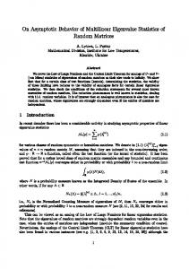
Wehrhahn and Ogawa (1978). A drawback of these papers is that the conclusions drawn are based on simulations and numerical evaluations of the rather complicated exact probabilities. However, in addition to numerical work, it would be nice if we could get insight in a qualitative way why this failure occurs and quantitatively how large it is. Hence, we would like to have some simple approximations that can be used to gain more insight in the functional relationships between various parameters. A first step is to apply some standard asymptotics, from which the following picture evolves. Although the sample sizes tend to infinity in an asymptotic approach, the F -test should attain a prescribed power for a given level, and hence we cannot consider fixed alternatives, since then the power would tend to one as the sample sizes tend to infinity, but we have to consider Pitman alternatives. For such nearby alternatives, the variance ratio tends to one as the sample sizes increase. But under these circumstances, the level of the t-test will nicely tend to the prescribed nominal value and the problem resolves. Hence simple asymptotics, just as the intuitive reasoning mentioned above, completely overlooks the only too real difficulties established in practice. In this chapter we show that application of second-order asymptotics fortunately does suffice to make matters transparent. We derive a simple expression for the minimal sample size that would be required to trust the intuitive justification for a preliminary F -test. These expressions make clear the relations between sample sizes, variance ratios and levels involved, thus giving the qualitative insight. Moreover, quantitatively it is also evident from these expressions that the sample sizes required are indeed typically large (and quite often huge). Before dealing with the two-sample case in Section 2.3, we begin by studying in Section 2.2 the simpler one-sample version of the problem. Although not that often mentioned in textbooks or literature, a similar situation occurs there. If the variance is known to be equal to a certain value, one might prefer to use the Gauss test instead of the ordinary one-sample t-test for testing the hypothesis of main interest concerning the mean. A preliminary χ2 -test can be used to test the assumption about the variance. It turns out that for the power of the preliminary test, first-order methods still suffice, but that in particular the approximation for the level of the preferred main test has to be improved by use of second-order asymptotics. Some figures are added to demonstrate that the approximations work very well.

2.2

The one-sample case

In this section we consider the one-sample counterpart of the more familiar two-sample case mentioned. From a practical point of view, this case is only marginally interesting. However, as it is considerably simpler, its study will help our understanding of what is going on, which is precisely our aim. Let X1 , . . . , Xn be independent identically distributed (i.i.d.) random variables

2.2. The one-sample case

13

(r.v.’s) from the N (µ, σ2 )-distribution. Suppose we are interested in the mean, and want to test the main null hypothesis H0 : µ = µ0 against one-sided alternatives H1 : µ > µ0 at level α. To decide what test we shall use for this testing problem, we wonder whether we may assume the variance to be equal to some known value σ02 . This assumption, which clearly forms the analogue of the equality-of-variances assumption in the two-sample case, can be tested by a two-sided χ2 -test at level δ, ¯ 0 : σ = σ0 in favor of H ¯ 1 : σ 6= σ0 for either small or large say. This test rejects H values of the test statistic based on the sample variance S 2 , i.e. when (n − 1)S 2 < χ2n−1,1−δ/2 σ02

or

> χ2n−1,δ/2 ,

(2.2.1)

where for example χ2n−1,δ/2 denotes the upper (δ/2)-point of the chi-squared distribution with (n − 1) degrees of freedom (df). If this preliminary test does not reject, we feel encouraged to apply the Gauss test for the main testing problem on the mean. Then H0 is rejected when ¯ − µ0 ) n1/2 (X > uα , σ0

(2.2.2)

¯ is the sample mean and uα = Φ−1 (1−α) is the upper α-point of the standard where X normal distribution function Φ. ¯ 0 , then an alternative test for the mean If, however, the preliminary test rejects H has to be used. An obvious choice is the t-test, which uses an estimator S for σ, and which hence rejects when ¯ − µ0 ) n1/2 (X > tn−1,α S

(2.2.3)

with tn−1,α denoting the upper α-point of the t-distribution with (n − 1) df. For the procedure described above we study the power of the preliminary test in relation to the actual size of the Gauss test. We first specify what we consider to be an intolerable size for the Gauss test, and give an exact expression for the corresponding variance ratio by which this is caused. Subsequently, we consider the power of the preliminary test for these variance ratios and give a criterion to quantify when it is considered to be sufficiently large. The exact sample size needed to meet this criterion is evaluated numerically. After this, we derive approximations to get the desired theoretical insight. The actual size of the Gauss test exactly equals α ˜ = 1 − Φ(uα /r1/2 ),

(2.2.4)

where r = σ2 /σ02 . Suppose we define a tolerable deviation from the nominal level by stipulating that the relative error h(r) = (˜ α − α)/α in the size should satisfy |h(r)| ≤ |ε|,

(2.2.5)

14


for some given, small ε. Taking e.g. ε = ±0.4 means that at a nominal level of 5% a range from 3% to 7% is allowed. Clearly, as h is an increasing function of r, attention will focus on the just tolerable values re , for which h(re ) = ε holds exactly. It follows immediately that re = u2α /u2α(1+ε) .

(2.2.6)

Hence, for variance ratios r larger than the value of re corresponding to positive ε, or smaller than the value re corresponding to negative ε, the Gauss test is considered unacceptable. ¯ 0 : σ = σ0 . For a given Now consider the power of the preliminary χ2 -test for H level δ it can be considered as a function of the sample size n and the variance ratio r and will be denoted by π(n, r). It equals π(n, r) = 1 − P (χ2n−1 < χ2n−1,δ/2 /r) + P (χ2n−1 < χ2n−1,1−δ/2 /r),

(2.2.7)

where χ2n−1 is a r.v. with a chi-squared distribution with (n − 1) df. Again a bound has to be prescribed. Suppose we define sufficiently high power for this test to mean that for all variance ratios r for which the size of the Gauss test violates (2.2.5), we should have a power of at least π0 , i.e. π(n, r) ≥ π0 ,

(2.2.8)

for some given, sufficiently large π0 . A minimal requirement would seem to be π0 ≥ 0.50. Since the variance ratios violating (2.2.5) satisfy |r − 1| > |re − 1|, it follows from the monotonicity of the power in |r − 1| that it suffices to require (2.2.8) for re . Hence n should simply satisfy π(n, re ) ≥ π0 .

(2.2.9)

Numerically, it is straightforward to obtain ne = ne (α, δ, ε, π0 ), the smallest integer-valued number n for which (2.2.9) holds. This is exactly the minimum sample size, needed to ensure a sufficiently high power (in the sense of (2.2.9)) in cases where deviations of the size of the Gauss test from the desired nominal level are no longer tolerable (in the sense of (2.2.5)). In Figure 2.2.1, among others, values of ne are presented for various α, δ, ε and π0 . From these results we readily infer that very large sample sizes are required. This is in agreement with the assertion of Markowski and Markowski (1990) for the two-sample case they studied. Moreover, ne is seen to vary widely as a function of its parameters. This makes it even more desirable to gain theoretical insight into the functional relationships involved, which is not given by the numerical results. To this end, we now derive some simple approximations based on asymptotics. For the probability in (2.2.4) that the Gauss test rejects, we can easily write down a Taylor expansion for r about 1. This leads to a second-order approximation for the actual size of the Gauss test, reading α ˜ = 1 − Φ(uα /r1/2 ) = α + 12 (r − 1)uα ϕ(uα ) + O (r − 1)2 , (2.2.10)


15

where ϕ = Φ0 denotes the density of the standard normal distribution. The fact that we expand here in terms of (r − 1) is justified by the fact that (r − 1) has to be of order n−1/2 (Pitman alternatives for the preliminary test). It will be immediately clear from expression (2.2.17) below, that for a different order the χ2 -test cannot achieve a prescribed power as n tends to infinity. Note that the result in (2.2.10) contains the more simple first-order approximation α ˜ = α + O(|r − 1|). However, this is clearly useless in the present context: it gives α ˜ ≈ α and thus h(r) ≈ 0, which means that (2.2.5) is never violated. Hence we really need the second-order version α ˜ ≈ α + 12 (r − 1)uα ϕ(uα ) from (2.2.10), which leads to h(r) = (˜ α − α)/α ≈ 1 (r − 1)u ϕ(u )/α. Replacing h(r) by this approximation in solving h(r) = ε leads α α 2 to the approximation r1 − 1 =

2εα uα ϕ(uα )

(2.2.11)

for re − 1 with re from (2.2.6). (Obviously, the step from (2.2.6) to (2.2.11) could have been made by direct analysis, but that would have been less illuminating). Next consider the power of the preliminary test. In order to approximate π(n, r), we can for example use that √ 2 χn − n −1/2 2 2 √ P ≤ z = Φ(z) − n (z − 1)ϕ(z) + O(n−1 ) 3 2n (2.2.12) = Φ(z) + O(n−1/2 ). The first approximation in (2.2.12) is a one-step Edgeworth expansion (cf. e.g. Feller (1971), p. 542), whereas the latter obviously is the ordinary normal approximation for a standardized χ2n r.v. Inversion gives the corresponding approximation for the percentile points, namely √ χ2n,δ/2 − n 2 2 √ = uδ/2 + n−1/2 (u − 1) + O(n−1 ) 3 δ/2 (2.2.13) 2n −1/2 ). = uδ/2 + O(n An alternative possibility is to use the Wilson-Hilferty approximation, based on the normal approximation for a transformation of the original variable (see Johnson and Kotz (1970), p. 176): r ! z 1/3 2 9n 2 P (χn ≤ z) ≈ Φ −1+ . (2.2.14) n 9n 2 This leads to r χ2n,δ/2

≈ n uδ/2

2 2 +1− 9n 9n

!3 (2.2.15)

16


as an approximation for the upper (δ/2)-point. We begin by simply applying the normal approximation from (2.2.12), Using (r − 1) = O(n−1/2 ) and writing the critical value, properly standardized under alternatives r 6= 1, as r χ2n−1,δ/2 /r − (n − 1) n p = uδ/2 − (r − 1) + O(n−1/2 ), 2 2(n − 1)

(2.2.16)

it follows that we may approximate the power π(n, r) of the preliminary test by r r n n 1 − Φ uδ/2 − (r − 1) + Φ −uδ/2 − (r − 1) + O(n−1/2 ). (2.2.17) 2 2 If we use (2.2.17) to solve π(n, re ) = π0 (cf. (2.2.9)), we obtain n ≈ n1 (re ) =

2(uδ/2 − uπ0 )2 (re − 1)2

(2.2.18)

under the typically reasonable assumption that one of the tails in (2.2.17) is negligible. Here we use “≈” to indicate that the number of observations n should be an integer, and hence equals the smallest integer above the value n1 (re ). Combination of this result with the approximation r1 from (2.2.11) for the just tolerable variance ratio, leads to the following approximation for ne 1 n1 = n1 (r1 ) = 2

(uδ/2 − uπ0 )uα ϕ(uα ) εα

2 .

(2.2.19)

Note that (2.2.19) indeed makes transparent the way in which the sample size depends on α, δ, ε and π0 . This is partly due to the fact that most of the parameters are separated. The expression does not only show that the required sample size increases as a function of the desired power π0 and decreases as a function of the nominal levels α and δ and the allowed deviation |ε| for the level of the Gauss test (as is intuitively clear), it also clarifies its behavior in a quantitative way. Moreover, the occurrence of ε2 α2 in the denominator of (2.2.19) explains why such large values occur. As mentioned before, Figure 2.2.1 presents ne for a number of configurations of the underlying parameters. To judge the performance of (2.2.19), we evaluated n1 for these cases as well. Comparison to the exact values shows that n1 follows these widely varying values remarkably well. In fact, the simple n1 ignores skewness effects and thus is an even function of ε (cf. (2.2.19)), while the exact ne typically is somewhat larger for positive ε than for negative ε. It turns out that the approximations nicely lie near the average of the corresponding two exact values. Only for the parameter combination δ = 0.5, π0 = 0.7 this does not hold. A closer look at the derivation of the approximation reveals the reason: the nominal level δ is very large compared to the required power π0 and therefore, neglecting one of the tails is not justified and leads to overestimation (cf. (2.2.17) and (2.2.18)).


17

1000

n e n 1 nwh

900 800 700

δ=0.05, π0=0.5

1000

800 700

δ=0.05, π0=0.7

600

600

500

500

400

400

300

300

200

200

100

100

0

α=0.05 α=0.05 α=0.1 α=0.1 α=0.05 α=0.05 α=0.1 α=0.1 |ε|=0.2 |ε|=0.4 |ε|=0.2 |ε|=0.4 |ε|=0.2 |ε|=0.4 |ε|=0.2 |ε|=0.4

1000

ne n1 nwh

900 800 700

δ=0.25, π0=0.7

δ=0.25, π0=0.9

n e n 1 nwh

900

0

δ=0.1, π0=0.6

δ=0.1, π0=0.8


600

ne n1 nwh

500

400

δ=0.5, π0=0.7

δ=0.5, π0=0.9

600 500

300

400 200

300 200

100

100 0


0


Figure 2.2.1 Minimal sample sizes for which π(n, re ) ≥ π0 , with h(re ) = ε, for various π0 , ε and levels α and δ of Gauss test and χ2 -test, respectively. Values of ne and nwh corresponding to positive and negative ε are denoted in the same bar, where the value for positive ε is the larger one; n1 is the same for positive and negative ε. Looking back, we observe that for the actual size of the Gauss test in (2.2.10) the second-order approximation was really necessary, whereas for the power of the preliminary test we could do with the first-order approximation in (2.2.12). Nevertheless, we did investigate whether further improvement could be achieved by using the refinement from (2.2.12) or the Wilson-Hilferty approximation from (2.2.14) after all. As the Wilson-Hilferty approximation coincides (not by accident!) with the onestep Edgeworth approximation to O(n−1 ), we only present the results for this first

18


possibility. The difference is completely negligible. If r > 1 (which corresponds to a positive value for ε), then we ignore the lower tail probability and solve 1 − P (χ2n−1 < χ2n−1,δ/2 /r) = 1 − Φ(uπ0 ). Using (2.2.14) and (2.2.15) gives a quadratic equation in root −f +

p 1 + f 2,

where f =

uδ/2 − r1/3 uπ0 . 2(1 − r1/3 )

(2.2.20) p 9(n − 1)/2, with positive

(2.2.21)

Similarly, when r < 1 (or ε negative), then we neglect the upper tail probability and find the same expression with f replaced by −f (since u1−γ = −uγ ). Noting that the first term (−f or +f ) is positive in both cases, substitution of r1 into f from (2.2.21) gives as an approximation for the required sample size nwh − 1 = nwh (r1 ) − 1 =

2 p 2 |f | + 1 + f 2 . 9

(2.2.22)

The results, also shown in Figure 2.2.1, are mixed. For α = 0.05, the values of nwh for negative and positive ε lie between the corresponding values for ne , with n1 lying nicely in between. Hence for α = 0.05 improvement indeed resulted. But for α = 0.10, the value we are primarily interested in, namely the maximum of the two, is generally overestimated by nwh , with a larger error than the error of n1 , which underestimates ne . However, more important to us is the fact that the expressions for nwh are much more complicated than the one for n1 . Hence, in view of the much greater simplicity of (2.2.19), refinements are not advised.

2.3

The two-sample case

We return to the main case, which is the two-sample situation. Consider two independent samples: X1 , . . . , Xm are i.i.d. r.v.’s from a N (µ1 , σ12 )-distribution and Y1 , . . . , Yn are i.i.d. r.v.’s from a N (µ2 , σ22 )-distribution. The question here is whether in testing the equality of means, we may trust the assumption that the variances are ¯ 0 : σ1 = σ2 against H ¯ 1 : σ1 6= σ2 , we equal. To test this assumption, i.e. to test H 2 2 apply a two-sided F -test at level δ, based on the ratio S1 /S2 of sample variances. ¯ 0 when This test rejects H S12 < Fm−1,n−1,1−δ/2 S22

or

> Fm−1,n−1,δ/2 ,

(2.3.1)

with Fm,n,γ denoting the upper γ-point of the F -distribution with m and n df in numerator and denominator, respectively.

2.3. The two-sample case

19

If no rejection is necessary, we dare to use the ordinary two-sample t-test, which assumes equality of variances. Then we reject H0 : µ1 = µ2 in favor of H1 : µ1 > µ2 if −1/2 ¯ − Y¯ ) 1 (X 1 + > tN −2,α , (2.3.2) S m n ¯ and Y¯ are the sample means, S 2 = (m − 1)S12 + (n − 1)S22 where N = m + n, X /(N − 2) is the pooled variance estimator, and tN −2,α is the upper α-point of the t-distribution with (N − 2) df. ¯ 0 , then one can use a modification of the twoIf the preliminary F -test rejects H sample t-test to test the equality of means, for example the one proposed by Welch (1937) and Satterthwaite (1946). Then H0 is rejected when ¯ − Y¯ ) (X

S12 S2 + 2 m n

−1/2 > tν,α ,

(2.3.3)

with ν given by ν=

S12 S22 + m n

2

S14 S24 + m2 (m − 1) n2 (n − 1)

.

(2.3.4)

Some straightforward modification suffices to apply the approach from the previous ˜ now be the actual size of the two-sample t-test section. Denote r = σ12 /σ22 , let α instead of the Gauss test and let π(N, r) refer to the power of the F -test instead of the χ2 -test. Then we can start looking again for approximations for the total sample size N required to detect harmful deviations from the equality-of-variances assumption with high probability. First determine for which variance ratios the size of the two-sample t-test is un¯ Y¯ ) and (S 2 , S 2 ), we obtain that satisfactory. Using the independence between (X, 1 2 ! 2 1/2 1 σ1 σ2 1 α ˜ = 1 − EΦ tN −2,α S 2 + + 2 , (2.3.5) m n m n which is indeed more complicated than its one-sample counterpart 1 − Φ(uα /r1/2 ). Fortunately, (2.3.5) can be simplified by expanding S 2 around its expected value and by using that tN −2,α = uα + O(N −1 ). Combined this leads to 1/2 ! (1 − λ)r + λ α ˜ = 1 − Φ uα + O(N −1 ), (2.3.6) (1 − λ) + λr where λ = n/N . Moreover, the correspondence between the one- and the two-sample case becomes visible: the choice λ = 1 reproduces 1 − Φ(uα /r1/2 ) in (2.3.6), while ¯ 2 > uα , which parallels (2.2.2). Note that this it transforms (2.3.2) into m1/2 X/σ approximation does not depend on the sample sizes anymore, and that we got rid

20


of the expectation. This simplifies the problem in such a way that from now on, we can proceed in the same way as in the one-sample case. Hence, we may separate the two problems of, firstly, finding variance ratios r for which the size of the ordinary ttest behaves unsatisfactorily, and secondly, by substitution of the just tolerable value re according to (2.2.5) into π(N, r), finding the minimum sample sizes N needed to achieve sufficiently large power in the sense of (2.2.9). As regards the error term in (2.3.6), note that it is of a smaller order than α ˜ − α = O(|r − 1|) = O(N −1/2 ) (cf. (2.2.10) and (2.2.17)). Indeed, a numerical check confirms that the error due to ignoring this O(N −1 )-term is negligible for the present purpose. Solving for re from h(re ) = ε while using this simplification and thus ignoring the O(N −1 )-term in (2.3.6), leads through the equation α ˜ = α(1 + ε) to ! 1/2 (1 − λ)re + λ = 1 − Φ(uα(1+ε) ), 1 − Φ uα (2.3.7) (1 − λ) + λre and thus to (1 − λ)(re − 1) + 1 = B, 1 + λ(re − 1)

(2.3.8)

where B = u2α(1+ε) /u2α . Hence re − 1 =

(B − 1) . (1 − 2λ) − (B − 1)λ

(2.3.9)

(Note that λ = 1 leads to re = B −1 , as in (2.2.6).) In analogy to (2.2.9), let Ne = Ne (α, δ, ε, π0 , λ) be the smallest N such that π(N, re ) ≥ π0 . Just like re , this Ne will be identified with the truly exact solution, as the difference is negligible. Next we turn to the problem of how to derive simple approximations to re , and, in particular, to Ne . As (B − 1) is small, the right-hand side of (2.3.9) may be approximated by (B − 1)/(1 − 2λ), unless (1 − 2λ) is small as well. However, it means no loss at all to exclude this possibility: when λ is close to 12 , the level of the t-test remains close to α. (Note that for λ = 12 , i.e. for equal sample sizes, the test statistics of the t-test and of the Satterthwaite test, which has approximately the correct level, coincide.) The problem we are interested in, of large deviations of level combined with small power will occur only for |1 − 2λ| bounded away from 0. As a second step, we expand (B − 1): as B = u2α(1+ε) /u2α , we observe that α(1 + ε) = 1 − Φ(uα B 1/2 ) = α − 12 (B − 1)uα ϕ(uα ) + O((B − 1)2 ). Hence (B − 1) approximately equals −(2εα)/(uα ϕ(uα )). Together with the first step, substitution now gives (cf. (2.2.11)) r1 − 1 =

εα (λ −

1 2 )uα ϕ(uα )

.

(2.3.10)

For the power π(N, r) of the preliminary F -test we again begin by applying the straightforward normal approximation. Let Fm,n be a r.v. which has an F distribution with m and n df in numerator and denominator, respectively, then

2.3. The two-sample case

21

Fm,n (and of course also Fm−1,n−1 ) asymptotically has a N (1, 2(m−1 + n−1 )) = N (1, 2{λ(1 − λ)N }−1 )-distribution. Hence π(N, r) is approximated by (cf. approximation (2.2.17) for the power in the one-sample case) ! ! 1/2 1/2 N λ(1 − λ) N λ(1 − λ) 1 − Φ uδ/2 − (r − 1) + Φ −uδ/2 − (r − 1) . 2 2 (2.3.11) Assuming that one of the tails may be neglected, this leads to (cf. (2.2.18)) N ≈ N1 (re ) =

2(uδ/2 − uπ0 )2 λ(1 − λ)(re − 1)2

(2.3.12)

as an approximate solution for the total sample size satisfying π(N, re ) = π0 . Combination of (2.3.10) and (2.3.12) gives as an approximation for Ne (cf. (2.2.19)): 2 N1 = N1 (r1 ) = λ(1 − λ)

(

(λ − 12 )(uδ/2 − uπ0 )uα ϕ(uα ) εα

)2 .

(2.3.13)

Just as in the one-sample case, the dependence on the underlying parameters is made quite clear, as well as the occurrence of large values of Ne . In particular, note how N1 /n1 = (2λ − 1)2 /{λ(1 − λ)} reflects the influence of the unbalancedness of the design. Figure 2.3.1, as a counterpart of Figure 2.2.1, depicts N1 as well as Ne . Since both N1 and Ne are symmetric around λ = 12 , it suffices to consider values of λ < 12 . The conclusion is similar: N1 manages to follow the wild behavior of Ne quite well, as an approximate average of the exact values for positive ε and negative ε. As concerns possible refinements, we point out that a well-known improvement consists of replacing Fm,n by log Fm,n . Using that log (F/r) ≈ F − 1 − log r, together with the normal approximation for F −1, it is easily verified that this entails replacing (r − 1) in (2.3.11) by log r, and thus replacing (2.3.12) by Nlog (re ) =

2(uδ/2 − uπ0 )2 λ(1 − λ) log2 re

,

(2.3.14)

which through combination with the approximate variance ratio r1 from (2.3.10) leads to an approximation Nlog = Nlog (r1 ). However, it turns out that the simple N1 outperforms this Nlog , rather than the other way around. This surprising phenomenon is easily explained by closer inspection of the errors involved. The inaccuracy of r1 w.r.t. re is largely compensated by the inaccuracy of N1 (re ) w.r.t. Ne . Such compensation is lacking for the more accurate approximation Nlog (re ) of Ne . Of course, Nlog (re ) itself, in combination with (2.3.9), also gives an explicit approximation for Ne , and this one is very accurate as can be seen from Figure 2.3.1. However, it is much less simple and transparent than N1 .

22


1400 δ=0.05, π0=0.5 1200

N e N 1 N (r ) log e

2500 δ=0.05, π0=0.7 2000

N e N 1 N (r ) log e

1000 1500

800 600

1000

400 500 200 0

α=0.05 α=0.05 α=0.05 α=0.05 α=0.1 α=0.1 α=0.1 α=0.1 |ε|=0.2 |ε|=0.2 |ε|=0.4 |ε|=0.4 |ε|=0.2 |ε|=0.2 |ε|=0.4 |ε|=0.4 λ=0.2 λ=0.3 λ=0.2 λ=0.3 λ=0.2 λ=0.3 λ=0.2 λ=0.3

1000 900 800

δ=0.25, π0=0.7

Ne N 1 N (r ) log e

0


2500 δ=0.25, π0=0.9 2000

Ne N 1 N (r ) log e

700 600

1500

500 400

1000

300 200

500

100 0


0


Figure 2.3.1 Minimal sample sizes for which π(N, re ) ≥ π0 , with h(re ) = ε, for various π0 , ε and levels α and δ of t-test and F -test, respectively, and sample size ratios λ < 12 . Values of Ne and Nlog (re ) corresponding to positive and negative ε are denoted in the same bar, where the value for positive ε is the larger one; N1 is the same for positive as for negative ε.

Chapter 3

Size and power of the pre-test procedure for the normal oneand two-sample problem 3.1

Introduction

In this chapter we further analyze the pre-test procedure for the normal one- and two-sample problem from Chapter 2. Let us briefly recall the procedure. In the twosample case, a preliminary F -test is applied in the first step to check whether the variances of the two normal samples are equal. If the F -test does not reject, then in the second step the equality of variances is taken for granted and the simple twosample t-test is applied to test the equality of means. If the F -test does reject, then we use the more complicated Welch-Satterthwaite test. The idea is quite clear: there is a natural inclination to stick to the standard and efficient t-test as long as possible. The F -test is supposed to single out deviations from the homogeneity-of-variances assumption that would lead to unacceptable deviations from the nominal level of the t-test. In the one-sample case the F -, t- and Welch-Satterthwaite test are replaced by the χ2 -, Gauss and one-sample t-test, respectively. Although the method described above is mentioned in numerous textbooks on statistics, almost no attention is paid to the behavior of the pre-test procedure. This suggests that most writers think that the procedure works well (and their readers too!). However, there are some questionable aspects about such pre-test procedures. The preliminary F -test may fail to reject, leading to application of the two-sample ttest while the essential assumption of equal variances is violated, and hence to serious deviations in size with respect to the prescribed level. Furthermore, the repeated use of the same data introduces correlations which influence size and power of the combined procedure. Contrary to the implicit optimistic view of textbooks, there are some papers on the 23

24

Chapter 3. Size and power of the pre-test procedure for the normal ...

subject that are in sharp contrast with this optimism. Related to the first aspect are the numerical results of Markowski and Markowski (1990), which show that for sample sizes occurring in practice, typically the F -test has low power against deviations that are sufficiently large to cause unacceptable departures from the nominal level of the ttest. Hence this first look at matters is not exactly reassuring. This phenomenon has been further analyzed and explained using second-order asymptotics in the previous chapter. The preceding results are related indirectly to the problem, since they only look at the first aspect, the relation between failing of the preliminary test and the resulting violation of the level of the main test. More direct results, which also incorporate the second aspect, the correlation between the tests, are also available. Moser, Stevens, and Watts (1989) have done considerable numerical work considering a variety of combinations of the parameters involved. They conclude that whenever the t-test is unreliable with respect to size, the same may hold for the combined procedure, and therefore they advocate to always use the alternative test. Their numerical results are very interesting, but do not give much insight in the behavior of actual size and power as functions of all the parameters involved. Their conclusion is clear (“always apply the Welch-Satterthwaite test”), but still many practitioners will prefer the simpler t-test if anyhow possible. To answer questions like “how wrong can it be to follow the textbooks” and “what is the best level for the preliminary test”, a simple and transparent formula for the actual size and power of the combined procedure is needed. In view of the above, it seems worthwhile to obtain insight in a qualitative way why the combined procedure fails to live up to expectations as indicated by the papers mentioned above. Moreover, it would also be nice to have quantitative guidelines on where and to what extent problems will occur. Instead of doing additional numerical work and trying to get the underlying structure in an experimental way, we apply asymptotic methods to express the actual size and power as functions of the parameters involved: the nominal sizes of the preliminary test and the other tests, the total number of observations and the ratio of the sample sizes of the two samples, the ratio of the variances of the two samples and (for the power) the distance between the means of the two samples. With so many parameters it is far from easy (if at all possible) to uncover the structure using only numerical results. To begin with, however, we emphasize that first-order asymptotics will be of little help either. In the Pitman case of nearby alternatives for the preliminary F -test, the variance ratios tend to one as the sample sizes increase. In that case the standard t-test asymptotically agrees with the Welch-Satterthwaite test. In particular, its size will tend to the intended nominal value. Hence, no problem seems to be present. In this chapter we show that second-order asymptotics suffices to make clear what happens. An explicit second-order approximation for the size and power of the combined pre-test procedure is derived in Section 3.2. To make the underlying structure as clear as possible, we first consider the simpler one-sample analogue. This facilitates the treatment and understanding of the two-sample case which subsequently follows. In both cases, the resulting expression shows the dependence on the under-

3.2. Main results: difference in size and power

25

lying parameters in a straightforward manner, thus providing the desired qualitative insight. It also serves quite well for quantitative purposes, to study the magnitude of the deviations involved. It turns out that the correlation between the tests, which was not taken into account in the analysis of the previous chapter, partly (but not sufficiently!) compensates the effect of using the wrong test after an inappropriate decision (failure to reject) by the preliminary test. The consequences with respect to the actual size of the pre-test procedure are discussed in Section 3.3, whereas the effects on the power are the subject of Section 3.4. In these sections the applicability and the accuracy of the approximations are also illustrated by solving different quantitative questions. The chapter is concluded with Section 3.5, where some comments are given about the methods used, as well as about possible refinements.

3.2

Main results: difference in size and power

3.2.1

The one-sample case

First we consider the one-sample analogue of the two-sample case from Section 3.1. As it is simpler, the desired insight is obtained rather easily, after which generalization to the case of main interest follows in a straightforward manner. Let X1 , . . . , Xm be i.i.d. r.v.’s from the N (µ, σ2 )-distribution. Under the assumption σ = σ0 , we test H0 : µ = µ0 against H1 : µ > µ0 at level α by applying the Gauss test, which rejects if ¯ − µ0 ) m1/2 (X > uα , σ0

(3.2.1)

¯ is the sample mean and uα = Φ−1 (1−α) is the upper α-point of the standard where X normal distribution function Φ. Without such an assumption about σ, our alternative procedure will of course be the one-sample t-test, which rejects if ¯ − µ0 ) m1/2 (X > tm−1,α , S

(3.2.2)

where S 2 is the sample variance and tm−1,α is the upper α-point of the t-distribution ¯ 0 : σ = σ0 , we apply a two-sided χ2 -test with (m − 1) df. As a preliminary test for H at level δ, which rejects if (m − 1)S 2 > χ2m−1,δ/2 σ02

or

< χ2m−1,1−δ/2 ,

(3.2.3)

where χ2m−1,δ/2 (χ2m−1,1−δ/2 ) is the upper (lower) (δ/2)-point of the χ2 -distribution ¯ 0 , we subsequently use the t-test; with (m − 1) df. If this preliminary test rejects H otherwise the Gauss test is applied. Let Pµ,σ denote that Xi , i = 1, . . . , m has a N (µ, σ2 )-distribution, and denote the probability that the just described pre-test procedure rejects H0 by π ∗ . (Of

26


course, it is a function of the actual values of the mean and variance. Later we will explicitly express this dependence as a function of the parameters which define the Pitman alternatives for µ and σ.) Clearly π ∗ is the following sum of two bivariate probabilities 1/2 ¯ 1/2 ¯ m (X − µ0 ) m (X − µ0 ) π∗ = Pµ,σ > tm−1,α , Ac , > uα , A + Pµ,σ σ0 S (3.2.4) where A = {χ2m−1,1−δ/2
uα , A − Pµ,σ > tm−1,α , A . σ0 S (3.2.6) This will be useful in the proof of the main result, given in the next theorem. In the theorem we give an asymptotic approximation for the difference π ∗ − π ˜ as a function of the actual underlying mean and variance, the sample size m, and the nominal levels α and δ for the two main tests and for the preliminary test, respectively. To this end, we consider Pitman alternatives, not only for H0 : µ = µ0 , but also ¯ 0 : σ = σ0 . To be more precise, we let without loss of generality µ0 = 0 and for H σ0 = 1 and we suppose that for m → ∞ we have µ = bm−1/2 ,

σ = 1 + c(2m)−1/2 ,

(3.2.7)

for some constants b and c with b ≥ 0. The normalization for σ is chosen for convenience in the result. Then we obtain, with ϕ = Φ0 Theorem 3.2.1 Under (3.2.7), the difference π ∗ − π ˜ from (3.2.6) satisfies π∗ (b, c) − π ˜ (b, c) = (2m)−1/2 uα ϕ(uα − b)h(c, uδ/2 ) + O(m−1 ),

(3.2.8)

h(x, y) = x{Φ(y − x) − Φ(−y − x)} − {ϕ(y − x) − ϕ(−y − x)}.

(3.2.9)

where


27

Proof. To shorten notation, write the acceptance region A (cf. (3.2.5)) as {aL < S < aU } (hence e.g. aU = {χ2m−1,δ/2 /(m − 1)}1/2 ). First conditioning on S in (3.2.6) and taking the expectation with respect to S, it follows that tm−1,α S − b uα − b π∗ − π ˜=E Φ −Φ I(aL ,aU ) (S). (3.2.10) σ σ Now we expand the part in brackets. As tm−1,α = uα + O(m−1 ), we obtain in view of (3.2.7), according to which σ = 1 + O(m−1/2 ) tm−1,α S − b uα − b Φ −Φ = uα ϕ(uα − b)(S − 1) + O(m−1 + (S − 1)2 ). σ σ (3.2.11) Combination of (3.2.10) and (3.2.11) leads to ˜ = uα ϕ(uα − b)E(S − 1)I(aL ,aU ) (S) + O(m−1 + E(S − 1)2 ). π∗ − π

(3.2.12)

The factor E(S − 1)I(aL ,aU ) (S) can be approximated by using the standard normal p approximation to the distribution of S˜ = (S − ES)/ var(S). Then we get, with ˜ a ˜L and a ˜U the ˜U = p boundaries of the acceptance region written in terms of S (e.g. a (aU − ES)/ var(S)) p ˜ E(S − 1)I(aL ,aU ) (S) = E S˜ var(S) + ES − 1 I(ãL ,ãU ) (S) n o = (ES − 1) Φ (˜ aU ) − Φ (˜ aL ) + O(m−1/2 ) n o p − var(S) ϕ (˜ aU ) − ϕ (˜ aL ) + O(m−1/2 ) .

(3.2.13)

Remains to evaluate this expression. For evaluation of the moments, we may use the following expansion 3 o1/2 1 S2 2 S 2 n S2 S 1 S2 − 1 = 1 + − 1 − − 1 + O − 1 = 1+ . σ σ2 2 σ2 8 σ2 σ2 3 2 Noting that E S 2 /σ2 − 1 = 0, E S 2 /σ2 − 1 = 2(m − 1)−1 and E S 2 /σ2 − 1 = O(m−3/2 ) and hence E(S/σ) = 1 − (4m)−1 + O(m−3/2 ), var(S/σ) = (2m)−1 + O(m−3/2 ), we find in view of (3.2.7) that ES = σ + O(m−1 ) = 1 + c(2m)−1/2 + O(m−1 ), p var(S) = (2m)−1/2 + O(m−1 ).

(3.2.14)

From the normal approximation of the χ2 -percentile points (cf. also (2.2.13)), it is easy to derive the approximations for aL and aU . For aU we get aU = 1 + uδ/2 (2m)−1/2 + O(m−1 ), for aL the same expression with uδ/2 replaced by −uδ/2 . Hence a ˜L = −uδ/2 − c + O(m−1/2 )

and a ˜U = uδ/2 − c + O(m−1/2 ).

(3.2.15)

28


Finally, combination of (3.2.12) and (3.2.13) with (3.2.14) and (3.2.15) yields the desired result. 2

3.2.2

The two-sample case

Next we return to the situation of main interest, which is the two-sample case. Let X1 , . . . , Xm and Y1 , . . . , Yn be independent r.v.’s, the Xi from N (µ1 , σ12 ), i = 1, . . . , m and the Yj from N (µ2 , σ22 ), j = 1, . . . , n. A two-sided F -test, based on the ¯ 0 : σ1 = σ2 . This test ratio S12 /S22 of sample variances, is applied at level δ to test H ¯ 0 when rejects H S12 < Fm−1,n−1,1−δ/2 S22

or

> Fm−1,n−1,δ/2 ,

(3.2.16)

with Fm−1,n−1,δ/2 (Fm−1,n−1,1−δ/2 ) denoting the upper (lower) (δ/2)-point of the F distribution with (m − 1) and (n − 1) df in numerator and denominator, respectively. As long as no rejection is needed, we use the standard two-sample t-test, which rejects H0 : µ1 = µ2 at level α in favor of H1 : µ1 > µ2 if ¯ − Y¯ ) (X S

1 1 + m n

−1/2 > tN −2,α ,

(3.2.17)

¯ and Y¯ are the sample means and S 2 = {(m − 1)S12 + where N = m + n, X 2 ¯ 0 has to be rejected, we resort to the approxi(n − 1)S2 }/(N − 2). However, if H mate Welch-Satterthwaite t-test, which rejects if ¯ − Y¯ X > tν,α , S22 /n)1/2

(3.2.18)

(S12 /m + where ν=

S12 S22 + m n

2

S14 S24 + m2 (m − 1) n2 (n − 1)

.

Again π ∗ is the power of the combined procedure, which can easily be written down analogous to expression (3.2.4) for the one-sample case, but now π, π ˜ and π ¯ stand for the powers of the two-sample t-, the Welch-Satterthwaite and the F -test. Without loss of generality we let σ2 = 1 and, in analogy to (3.2.7), assume that for some constants b and c with b ≥ 0 µ1 − µ2 = b(κN )−1/2 ,

σ1 = 1 + c(2κN )−1/2 ,

(3.2.19)

where κ = λ(1 − λ), with λ = n/N (and thus (κN )−1/2 = (1/m + 1/n) have that

1/2

). Then we


29

Theorem 3.2.2 Under (3.2.19), the difference π ∗ − π ˜ satisfies π∗ (b, c) − π ˜ (b, c) = (2λ − 1)(2κN )−1/2 uα ϕ(uα − b)h(c, uδ/2 ) + O(N −1 ), (3.2.20) with h as in (3.2.9). Proof. We extend the proof of Theorem 3.2.1. From (3.2.17) and (3.2.18) it follows ˜ equals that we obtain in analogy to (3.2.10) that π ∗ − π ( E

! b(κN )−1/2 − Φ tN −2,α − 2 (σ1 /m + σ22 /n)1/2 !) 2 1/2 2 b(κN )−1/2 S1 /m + S22 /n S1 I − , + Φ tν,α (aL ,aU ) σ12 /m + σ22 /n S22 (σ12 /m + σ22 /n)1/2 (3.2.21)

S2 (σ12 /m + σ22 /n)

1 1 + m n

1/2

where now aU and aL correspond to the upper and lower (δ/2)-points of the Fm−1,n−1 distribution (hence e.g. aU = Fm−1,n−1,δ/2 ). A step similar to (3.2.11), but slightly more complicated, shows that the leading term of π ∗ − π ˜ will be contained in 2 2 S1 S1 1 − 1 I(aL ,aU ) . (3.2.22) 2 (2λ − 1)uα ϕ(uα − b)E S22 S22 The desired result (3.2.20) then follows by applying (3.2.13) with S replaced by S12 /S22 and by using some straightforward results like ES12 /S22 = σ12 /σ22 (1 + O(N −1 )) = 1 + c{2/(κN )}1/2 + O(N −1 ), var(S12 /S22 ) = 2/(κN )(1 + O(N −1/2 )),

(3.2.23)

aU = 1 + uδ/2 {2/(κN )}1/2 + O(N −1 ), which follow from expectation, variance and normal approximation of an F distributed variable, respectively. 2 Remark 3.2.1 Comparison of (3.2.19) and (3.2.20) to (3.2.7) and (3.2.8), respectively, shows that the two-sample case is indeed closely related to the more transparent one-sample case: (κN )−1 = m−1 + n−1 replaces m−1 from the former case, while the factor (2λ − 1)κ−1/2 in (3.2.20) represents the unbalance of the design. In fact, the limiting situation n = ∞ exactly coincides with the one-sample case. Note that the two-sample t-test corresponds to the Gauss test in the one-sample case, rather than to the one-sample t-test.

30


Remark 3.2.2 Up to now we have restricted attention to the one-sided test of the main null hypothesis H0 . It is easily verified that for the two-sided version of the test, results similar to (3.2.8) and (3.2.20) will hold. To be precise, it suffices to put in a factor 2 (to account for both tails) and to replace α by α/2. (Hence the expression for the relative error (π ∗ (0, c) − α)/α of the size in the two-sided case is the same as in the one-sided case with therein α replaced by α/2.) Remark 3.2.3 We should bear in mind that the approximation (3.2.8) or (3.2.20) is no goal in itself, but only serves to provide answers about questions concerning when and to what extent deviations can occur. Hence we shall postpone details about numerical accuracy mainly to the next section. Here we merely remark that the approximations seem sufficiently adequate for our purposes. For example, (3.2.8) leads for m = 25 and α = 0.05 to relative errors in the size of about 3% to 4%. Moreover, the magnitude of the error indeed behaves like order m−1 , as suggested by (3.2.8).

3.3

Consequences for the actual size

In this section we consider the null hypothesis case, where b from (3.2.7) and (3.2.19) equals zero and π ∗ − π ˜ from (3.2.8) and (3.2.20) thus reduces (up to the order given) to π ∗ (0, c) − α, the departure from the nominal level. We begin by noting that the expressions in (3.2.8) and (3.2.20) nicely separate the effects of the parameters involved. Clearly, the error π ∗ (0, c) − α decreases at rate m−1/2 or (κN )−1/2 as the sample sizes increase. It also tends to 0 for α ↓ 0, but uα ϕ(uα )/α behaves like u2α in this case, and thus the relative error increases. For the two-sample case, the factor (2λ − 1)κ−1/2 in (3.2.20) represents the unbalancedness of the design. In particular, it follows that for m = n the error is 0 to second order as well. This is in agreement with the conclusion from Markowski and Markowski (1990) and Moser, Stevens, and Watts (1989), according to which the problem vanishes for (nearly) equal sample sizes. Moreover, (2λ − 1)κ−1/2 = 2(λ − 12 ){ 41 − (λ − 12 )2 }−1/2 and hence, the farther away λ is from 12 , the larger this factor is. After these simple relations for m, n, and α, it remains to study the dependence on δ and c, which is contained in h(c, uδ/2 ) from (3.2.8). As our starting point we shall use the following link to the preliminary approach by Markowski and Markowski (1990), which was further analyzed in Chapter 2. If the dependence between the preliminary test and the subsequent tests is ignored, the right-hand side of (3.2.6) reduces to (π − π ˜ )(1 − π ¯ ), which in the present situation equals (π(0, c) − α)(1 − π ¯ (0, c)). Hence this indeed suggests that control of the error π ∗ (0, c) − α requires that either the error π(0, c) − α in the size of the Gauss test or two-sample t-test, respectively, is small, or that the power π ¯ is large for c 6= 0. The connection to the present approach now simply is the following: write h =

3.3. Consequences for the actual size

31

h1 + h2 , in which h1 (x, y) = x{Φ(y − x) − Φ(−y − x)},

(3.3.1)

h2 (x, y) = ϕ(y + x) − ϕ(y − x), then (π − π ˜ )(1 − π ¯ ) is nothing but the expression in either (3.2.8) or (3.2.20) if we replace h by h1 . Hence the thus ignored contribution by h2 represents the correction required by the dependence between the test statistics. The behavior of h and the role of h1 and h2 can be analyzed as follows. Note that h1 (c, uδ/2 ) and h2 (c, uδ/2 ) are odd in c, so it suffices to consider c ≥ 0. For all c ≥ 0 and uδ/2 ≥ 0, we have h1 ≥ 0 and h2 ≤ 0. Since h(c, 0) = h1 (c, 0) = h2 (c, 0) = 0 for all c, and h = h1 + h2 increases in uδ/2 for c ≥ 0, the sum h ≥ 0 for all uδ/2 ≥ 0 and c ≥ 0. Hence, 0 ≤ h ≤ h1 . Moreover, since h(0, uδ/2 ) = 0 and limc→∞ h(c, uδ/2 ) = 0 while h(c, uδ/2 ) ≥ 0 for all uδ/2 and c ≥ 0, the function h has a maximum for some c ≥ 0. This also applies to h1 . The statistical implications of these properties are illustrated in Figure 3.3.1. If the Gauss test or two-sample t-test, respectively, is directly applied without preliminary test (δ = 0), then we have h(c, uδ/2 ) = c which would lead to dramatic deviations of the size, since then the deviation grows linearly in c. Application of the pre-test procedure (δ > 0) improves matters. Then the violation of the level is smaller than that of the Gauss or two-sample t-test, for two reasons. The first reason for this is that the factor (1 − π ¯ ) starts to play a role. Instead of the linear function c, we now get the function h1 , in which c is multiplied by the acceptance probability of the preliminary test (1 − π ¯ ) which is smaller than 1. Contrary to the linear function c, the function h1 reaches a maximum for some c ≥ 0, and then decreases, reflecting that at some point the power of the preliminary test becomes large enough to detect harmful deviations from the assumptions about the variance(s). Secondly, the effect of the dependence between the tests (which was not taken into account previously) leads to a further reduction of the error through replacement of h1 by h. In Figure 3.3.1 the functions are sketched for δ = 0.05. Apart from the qualitative properties, derived in the foregoing from (3.2.8) or (3.2.20), also many quantitative questions can be answered from these results. We mention a few typical questions of increasing complexity and present also some numerical results to illustrate the accuracy of the approximations. Note that π ˜ (0, c) = α + O(N −1 ). Question 1. What is the error of the size if the nominal level α = 0.05, m = 20, n = 40, σ1 = 1.3, σ2 = 1 and δ = 0.05? We get λ = 23 , κ = 29 , N = 60, uα = 1.645, c = 1.55 and uδ/2 = 1.96. Inserting this in (3.2.20) yields π ∗ (0, 1.55) ≈ 0.0572. The numerical value of π ∗ (0, 1.55) equals 0.0582. Replacing α = 0.05 by α = 0.01 we get π ∗ (0, 1.55) ≈ 0.0126 with corresponding numerical value 0.0137.

32

Chapter 3. Size and power of the pre-test procedure for the normal ... 2.5

2

c

1.5

h1 (c, 1.96)

1

h(c, 1.96) 0.5

0 0

0.5

1

c

1.5

2

2.5

Figure 3.3.1 Functions c, h1 and h as a function of c for δ = 0.05.

Question 2. How large do we have to take N in order that the absolute error of the size is at most 0.01 for all λ with 0.2 ≤ λ ≤ 0.8, when c = 1.55, α = 0.05 and δ = 0.05? The approximation of the absolute error, using the right-hand side of (3.2.20), is an increasing function of |λ − 12 |. Hence, we should consider λ = 0.2 or 0.8. We get |π ∗ (0, 1.55) − α| ≈ 0.1179 N −1/2 , implying N = 139. The numerical value for m = 28, n = 111 of π ∗ (0, 1.55) is 0.0612, while for m = 111 and n = 28 we get 0.0407 numerically. Question 3. How large do we have to take δ in order that the (absolute) error of the size is at most 0.005 for α = 0.05, m = 20, n = 40, σ1 = 1.3 and σ2 = 1? Instead of δ being prescribed (cf. Question 1), we now know the maximum deviation from the size which is allowed, and have to choose δ. Substituting λ = 23 , κ = 29 , N = 60, uα = 1.645 and c = 1.55 in (3.2.20), it follows that we have to solve 0.01095 h(1.55, uδ/2 ) ≤ 0.005. This can be done numerically, but also some further approximations can be applied. Firstly, we may ignore Φ(−uδ/2 − 1.55) and ϕ(−uδ/2 − 1.55) (from the lower tail of the acceptance probability of the preliminary test), since they will be very small. Secondly, for uδ/2 not too far from 1.55 we may replace Φ(uδ/2 − c) by its first-order Taylor expansion Φ(0) + (uδ/2 − c)ϕ(0) and also ϕ(uδ/2 − c) by ϕ(0). Hence, we solve 0.01095[1.55{ 21 + (uδ/2 − 1.55)ϕ(0)} − ϕ(0)] ≤ 0.005, which is linear in uδ/2 , yielding uδ/2 ≤ 1.68. The numerical value of π ∗ (0, 1.55) for m = 20, n = 40, σ1 = 1.3, σ2 = 1, α = 0.05 and δ = 0.093 (corresponding to

3.4. Consequences for the actual power

33

uδ/2 = 1.68) is 0.0561. Question 4. What is the maximal error of the size if α = 0.05, m = 20, n = 40 and δ = 0.05? (cf. Question 1). Now we have to deal with maxc h(c, 1.96). The maximum equals 0.6581 and the maximum is attained at c = 1.4583, cf. also Figure 3.3.1. Therefore the error, maximized over c, equals 0.0072 according to (3.2.20). The numerical value of π ∗ (0, c)−α at c = 1.4583 is 0.0081. Replacing δ = 0.05 by δ = 0.25 we get maxc h(c, 1.15) = 0.1922, which is attained at c = 1.1431. The resulting error, according to (3.2.20), equals 0.0021. The numerical value of π ∗ (0, c) − α at c = 1.1431 is 0.0027. Question 5. What is the best level for the preliminary test if |(π ∗ (0, c) − α)/α| should not exceed some given ε > 0 (e.g. 0.20 leading to an actual size of either 2% or 3% for a nominal level α = 0.025) for all c? Let c∗ = c∗ (uδ/2 ) be the c that maximizes h(c, uδ/2 ) for given δ and h∗ (uδ/2 ) = ∗ h(c , uδ/2 ) the maximum value. Note that, as h itself decreases in δ, so does h∗ . By (3.2.20), δ should be sufficiently large to ensure that h∗ (uδ/2 ) ≤

ε(2κN )1/2 α . |2λ − 1|uα ϕ(uα )

(3.3.2)

To evaluate h∗ (uδ/2 ) we may use the following further approximation, cf. also Question 3. For uδ/2 ≥ 1 we have c∗ ≥ 1.1 (which can be checked empirically) and hence we ignore cΦ(−uδ/2 − c) and ϕ(−uδ/2 − c). Then c∗ = uδ/2 − g(1/uδ/2) with g = (ϕ/Φ)−1 and h∗ (uδ/2 ) = {uδ/2 [uδ/2 − g(1/uδ/2 )] − 1}ϕ(g(1/uδ/2 )). It turns out that for 1 ≤ uδ/2 ≤ 2.5 a good linear approximation is obtained by taking g(x) = 32 (1 − 54 x) and h∗ (x) = 35 x − 12 . Taking m = 20, n = 80, α = 0.025 and ε = 0.2, (3.3.2) reads as 35 uδ/2 − 12 ≤ 0.4115, yielding δ ≥ 0.129. The numerical value of π∗ (0, c) at c = uδ/2 − 32 (1 − 5/(4uδ/2 )) = 1.2534 equals 0.0315. It is seen from these examples that pretty good and very useful answers can be achieved for many questions in an easy way using Theorem 3.2.2. In a similar way Theorem 3.2.1 can be applied.

3.4

Consequences for the actual power

Here we can be quite brief, by virtue of the simplicity of the situation. From (3.2.20) it follows that for all c π∗ (b, c) − π ˜ (b, c) ϕ(uα − b) = + O(N −1/2 ). ∗ π (0, c) − α ϕ(uα )

(3.4.1)

Hence to first order the power difference is nothing but the size difference, inflated by a factor ϕ(uα − b)/ϕ(uα ). Clearly, this factor is always positive. It will typically be larger than 1, and it will reach its maximal value for b = uα , e.g. 3.9 if α = 0.05.

34


As expected, a gain in power is thus achieved by exceeding the nominal level under the null hypothesis. Likewise, if the procedure happens to be conservative, then a loss of power is sustained. However, it is not known beforehand which of the two will be the case. This pattern is of a general nature. For example, take the simpler situation of a single test statistic which has a distribution that converges to a normal one with expectation b and variance 1. For comparison one may think of the one-sample t-test in the one-sample case. Then we can also gain power by allowing a larger size, (which would be fair in the comparison with the pre-test procedure if we do allow it there), since a larger size will automatically lead to a larger power. Suppose we tolerate a size of α(1 + ε) instead of α, with ε = O(N −1/2 ). Then relation (3.4.1) also applies. However, the difference is that then the size will always be as large as α(1 + ε) (and the power difference will be in correspondence with this according to (3.4.1)), while in the pre-test procedure the actual size will typically be somewhere between α and α(1 + ε). In our application we can choose δ according to (3.3.2) to ensure that α(1 + ε) will be the worst possible case, attained for c∗ . To conclude this section, we answer a typical question (cf. the approach in Section 3.3). Question 6. What is the power difference π ∗ (b, c) − π ˜ (b, c) if the nominal level α = 0.05, m = 80, n = 20, c = −1, b = 1 and δ = 0.05? We get λ = 0.2, κ = 0.16, N = 100, uα = 1.645, σ1 = 0.823 and uδ/2 = 1.96. Inserting this in (3.2.20) yields π ∗ (1, −1) − π ˜ (1, −1) ≈ 0.0330. The numerical value of π ∗ (1, −1) − π ˜ (1, −1) = 0.0384.

3.5

Discussion of the methods used

In Section 3.2 we presented the main results, followed by the implications for size (Section 3.3) and power (Section 3.4). Here we conclude this chapter with some comments on the methods used and a few possible refinements. From the fact that the expression on the right-hand side of (3.2.8) is of order m−1/2 , it is evident that first-order asymptotics fails. Note that using (3.2.6) provides a considerable shortcut compared to using (3.2.4) together with separate second-order approximations for π, π ˜ and π ¯ . By taking the difference as in (3.2.6) the first-order terms, which are the same for π and π ˜ , immediately cancel. For 1 − π ¯ the first-order result Φ(uδ/2 − c) − Φ(−uδ/2 − c) suffices. Being multiplied with the expression for the difference between the main tests, this still leads to a second-order approximation for the whole procedure. By taking δ = 0 it follows that the leading term of π − π ˜ equals the expression in (3.2.8), with h(c, uδ/2 ) replaced by c. Hence the part of (3.2.8) corresponding to the first of the two terms of h, stands for (π − π ˜ )(1 − π ¯ ). This we encountered in Section 3.3 as an approximation to (3.2.6), obtained by ignoring the dependence between the t-test and the χ2 -test. Obviously, this defect has been repaired in (3.2.8) by taking the second term of h into account. This interaction term

3.5. Discussion of the methods used

35

vanishes for both δ = 0 (i.e. when π ¯ = 0 and thus π ∗ = π) and δ = 1 (¯ π = 1 and ∗ π =π ˜ ). Although the expression in (3.2.8) is asymptotically negligible from the point of view of first-order asymptotics, it is typically of a larger order of magnitude than the ordinary difference π − π ˜ when no heterogeneity of variances occurs. Indeed, for δ = 0 and c = 0, we get π − π ˜ = O(m−1 ) from (3.2.8). In fact, the deficiency of the t-test with respect to the Gauss test is known to equal 12 u2α (cf. Hodges and Lehmann (1970)). This effect, be it rather small, is visible in practice. In this light, it becomes understandable that the present effects, which are of order m−1/2 rather than of order m−1 , do cause problems for sample sizes occurring in practice. Without problem the term of order m−1 can be obtained in (3.2.8) by applying the Edgeworth expansion for the distribution function of S and expanding one step further in (3.2.11)-(3.2.13). However, the resulting expression, being a linear combination of Φ(k) (±uδ/2 − c), k = 0, 1, . . . , 4, is much more complicated than (3.2.8) and hence we refrain from giving it here, as our aim is to provide a simple description. A similar comment applies to attempts to use a better approximation to the χ2 -distribution, such as the one due to Wilson and Hilferty (see Johnson and Kotz (1970), p. 176). They suggest to treat ( ) r 2/3 S 2 9(n − 1) V = − 1− σ 9(n − 1) 2 as a standard normal r.v. (cf. also (2.2.14)). Unfortunately, this leads through (3.2.11) and (3.2.12) to dealing with a truncated moment of S = σ

( 1+

s 2 2 V − 9(n − 1) 9(n − 1)

)3/2 .

If we approximate this in turn by 1 + {2(n − 1)}−1/2 V , we end up with (3.2.8) again. As concerns bounds, note the following. If we do not approximate tm−1,α and σ as we did in (3.2.11), then we can approximate (3.2.10) by uα − b S uα ϕ E tm−1,α − I(aL ,aU ) (S). (3.5.1) σ σ σ instead of (3.2.12). Since for x and y both nonnegative (nonpositive), Φ(y) − Φ(x) − (y − x)ϕ(x) is nonpositive (nonnegative), this approximation serves in such situations as a bound for the power gain (or size difference) π ∗ − π ˜ . For example, under H0 we have b = 0 and (3.5.1) is an upper bound for π ∗ (0) − α. If b is sufficiently large then (tm−1,α S − b)/σ is nonpositive except for an exponentially small probability and (3.5.1) can be used to obtain a lower bound for π ∗ − π ˜ . Note that for evaluation of (3.5.1) both EI(aL ,aU ) (S) = 1 − π ¯ and E(S/σ)I(aL ,aU ) (S) can be found from χ2 or gamma-tables.

36


Chapter 4

Size and power of pre-test procedures for parametric models 4.1

Introduction

The analysis in Chapters 2 and 3 of the pre-test procedure for the normal one- and two-sample problem gave us considerable insight in its behavior and in the dependence of size and power on the several variables involved (sample sizes, nominal levels and real underlying means and variances). However, more general insight in the behavior of pre-test procedures for other situations is still lacking. In this chapter we extend our knowledge to pre-test procedures for general parametric densities. Suppose we have a density with two parameters, θ and τ , say. The main testing problem concerns a testing problem on θ, while τ is a nuisance parameter. The pretest procedure consists of a preliminary test on τ , to test whether it equals a given value or not, followed by a suitable test in the restricted family with the given value of τ in case the preliminary test does not reject, while otherwise the test on θ is performed in the complete family including the nuisance parameter. For each of the three testing problems in the given models, we define an appropriate class of tests, containing all standard first-order optimal tests for the problem under consideration. The idea of the procedure just described is of course that people prefer the test in the restricted model as long as possible, either because of the convenience of greater simplicity of the test in the smaller model, or because of a possibly higher power of the test for the restricted model compared to the alternative test, due to “knowing the value of the nuisance parameter”. It is the aim in this chapter to find an attractive expression that reveals the differences in size and power between the pre-test procedure and the one-stage test in the complete family. Concerning the methods we use to arrive at meaningful and transparent results, 37

38

Chapter 4. Size and power of pre-test procedures for parametric models

a few things can be noticed in advance. In the special case of normal distributions, which gives back precisely the one-sample problem of the previous chapter, the χ2 -test and the Gauss or one-sample t-test are asymptotically independent (to first order). In general, independence between the preliminary test and the main tests does not necessarily hold. However, if the preliminary test is already almost a test for the main problem, a two-step procedure is not very appealing: the two steps should not be mixed up too much. And more than that, if the correlations between the test statistic applied for the preliminary test and those for the main tests are not small, then the size of the pre-test procedure varies wildly and unacceptable violations of the prescribed level cannot be avoided. This conclusion follows already from first-order asymptotics and is presented in Section 4.2. Hence, pre-test procedures are only of interest if the correlations between the preliminary test and the main tests are small. Furthermore, if the correlation parameter is small, first-order asymptotics with respect to the sample size is of little help anymore, as will be explained in Section 4.2. Note that this was also the case in the special situation of normal distributions considered in Chapter 3. There the correlation parameter equals zero. Fortunately, secondorder asymptotics makes clear what is going on. However, second-order asymptotic analysis with respect to the sample size for a fixed value of the correlation parameter, is rather hopeless and will not lead to useful expressions. This problem is tackled by applying asymptotics not only with respect to the sample size, but also with respect to the correlation parameter. The more complicated second-order analysis is made more transparent by taking into account that the two main tests are tests for essentially the same testing problem (although in different models) and therefore have some common part. The remaining difference is small, partly due to considering a small correlation parameter, which is no restriction, as pointed out. This makes it possible to reduce the rather large number of terms in the second-order asymptotic expansions substantially. This argument is worked out in the first lemma in Section 4.2 and may be of independent interest. In the same section notations and conditions are gathered, and the classes of tests for each of the three testing problems are defined. Also a technical lemma is presented, due to Götze (1987) on Edgeworth expansions for bivariate U -statistics when dealing with probability measures depending on the number of observations. The use of second-order asymptotics implies that we have to deal with U -statistics, rather than with sums of i.i.d. r.v.’s. The evaluation of the power under local alternatives induces the dependence on the sample size for the involved probability measures. Section 4.3 contains the main results formulated in two theorems which are proved using the lemmas of Section 4.2. The (bivariate) Edgeworth expansions of the test statistics are presented, followed by a transparent expression for the difference in size and power between the pre-test procedure and the one-stage test in the complete family. This expression gives much insight in a qualitative and quantitative sense. It turns out that for all members of the class of test statistics the same expression holds, except for one quantity coming from the main test in the simpler model. In particular, it means that (up to the considered order) there is no difference between applying e.g. the locally most powerful test with the restricted or unrestricted max-

4.2. Notation, assumptions and preliminaries

39

imum likelihood estimator of the nuisance parameter inserted, the likelihood ratio test, Rao’s efficient score test or Wald’s test in the preliminary test on τ or in the testing problem on θ in the complete family. The implications of the main results are discussed in Section 4.4. It starts with a general discussion on the consequences for the actual size and power. It is noted that the family of distributions and the class of tests are involved through only four parameters. Regarding the hope for power gain, it turns out that it is in most cases not realistic, since the power change is often mainly nothing else but a factor times the size change. This implies that a higher power is almost only obtained if the size exceeds the nominal level. Moreover, a higher power at some value of the nuisance parameter goes hand in hand with a lower power at another value of the nuisance parameter, while the true value is unknown! After the general discussion, two important classes of distributions are considered: two-parameter exponential families and symmetric location-scale families. In a general symmetric location-scale family the approximation for the deviation from the nominal level of the pre-test procedure is very simple: it is the same as that for the normal case, except for a multiplicative constant. For several examples from these two classes of distributions, the accuracy of our approximations is seen from comparison with some numerical results.

4.2

Notation, assumptions and preliminaries

Let θ ∈ R, τ ∈ R, and let X1 , . . . , Xn be i.i.d. r.v.’s with density f (x; θ, τ ) with respect to some measure µ on the measurable space (X , A). Our main testing problem concerns testing H0 : θ = θ0 against H1 : θ > θ0 . If the nuisance parameter τ would be known and be equal to τ0 , say, we would test θ = θ0 in the family f (x; θ, τ0 ). If we are not sure that τ = τ0 , then we use a pre-test procedure and proceed with ¯ 0 : τ = τ0 against the following two steps. First, we perform a preliminary test of H ¯ ¯ H1 : τ 6= τ0 . Secondly, if H0 is not rejected, then we test H0 in the family f (x; θ, τ0 ); otherwise, we test H0 against H1 in the family f (x; θ, τ ). To define the tests of the separate testing problems we give some notation and state some regularity conditions. Without loss of generality let θ0 = 0 and τ0 = 0. As usual (θ, τ ) will denote the true value of the parameter as well as a variable in R2 . Its meaning is clear from the context. The regularity conditions should hold on an open subset Ω0 of the parameter space Ω ⊂ R2 , containing (0, 0). Since we only deal with local alternatives, attention is restricted to Ω0 . The regularity conditions are of the same type as those used in classical large sample theory, see e.g. Lehmann and Casella (1998), p. 462. (Ri)

The set A = {x ∈ X : f (x; θ, τ ) > 0} is independent of (θ, τ ), i.e. the distributions Pθ,τ of Xi have common support.

(Rii)

For every x ∈ A, (∂ i+j /∂θi ∂τ j )f (x; θ, τ ) exists for i, j = 0, 1, 2, 3, (i, j) 6=

40

Chapter 4. Size and power of pre-test procedures for parametric models (0, 0), and we write ∗ ψij (x; θ, τ ) =

(Riii)

(∂ i+j /∂θi ∂τ j )f (x; θ, τ ) . f (x; θ, τ )

For i, j = 0, 1, 2, 3, (i, j) 6= (0, 0), there exist functions Hij such that ∂ i+j sup i j f (x; θ, τ ) ≤ Hij (x) ∂θ ∂τ (θ,τ )∈Ω0 with

Z Hij (x)dµ(x) < ∞. A

(Riv)

The Fisher information matrix under (θ, τ ) = (0, 0) ! ! ∗ 2 ∗ ∗ ) Eψ10 ψ01 I11 I12 E(ψ10 I= = ∗ ∗ ∗ 2 I21 I22 Eψ10 ψ01 E(ψ01 ) is finite and positive definite.

∗ ∗ ∗ In order to simplify notation, we write ψij or ψij (X) for ψij (X; 0, 0). Expectations under the model f (x; θ, τ ) are denoted by Eθ,τ , but are abbreviated to E under (θ, τ ) = (0, 0). Furthermore, let −i/2 −j/2 I22 .

∗ (x; θ, τ )I11 ψij (x; θ, τ ) = ψij

By application of the dominated convergence theorem it follows from (Rii) and (Riii) that Eθ,τ ψij (X; θ, τ ) = 0

for i, j = 0, 1, 2, 3,

(i, j) 6= (0, 0).

(4.2.1)

This will be used many times with (θ, τ ) = (0, 0). The correlation coefficient of ψ10 (Xi ) and ψ01 (Xi ) under (θ, τ ) = (0, 0) is given by ρ = I12 (I11 I22 )−1/2 .

(4.2.2)

Define the so-called score functions under (0, 0) S = n−1/2

n X i=1

ψ10 (Xi ) and T = n−1/2

n X

ψ01 (Xi ).

(4.2.3)

i=1

The statistic S corresponds to the locally most powerful (LMP) test for testing θ = 0 in the family f (x; θ, 0). Other candidates for testing H0 are e.g. the likelihood ratio (LR) test, the test based on the maximum likelihood estimator (MLE) and


41

Wald’s test. These are first-order optimal tests, all having the same leading term, and can (up to order n−1/2 ) be written in the form ( ) n X −1/2 −1/2 S n k(Xi ) (4.2.4) SK = S + n i=1

with Ek = 0. Therefore, we use this class of test statistics for testing H0 : θ = 0 against H1 : θ > 0, rejecting for large values of SK. (Here “K” refers to the known value of τ .) In particular, we have for the tests mentioned LMP : k = 0 LR

:k=

1 2

2 3 ψ20 − (ψ10 − 1) + ( 13 Eψ10 − 12 Eψ10 ψ20 )ψ10

(4.2.5)

2 3 MLE : k = ψ20 − (ψ10 − 1) + (Eψ10 − 32 Eψ10 ψ20 )ψ10 2 3 Wald : k = ψ20 − (ψ10 − 1) + 12 (Eψ10 − Eψ10 ψ20 )ψ10 .

Note that Rao’s efficient score test coincides with the LMP test. In (4.2.5) the expec3 tations Eψ10 and Eψ10 ψ20 appear. Their existence will be amply guaranteed by the additional regularity conditions (Rv) and (Rvi), respectively, which will be needed at the end of this section. This remark will also apply to the expectations occurring in the second main test and the preliminary test. These tests are more familiar in case of two-sided alternatives. The one-sided forms as needed here are e.g. presented as directed versions in Barndorff-Nielsen and Cox . (1994), p. 82. A brief justification for LR is as follows. (We use “=” for approximately −1/2 .) Here we deal with testing in the family f (x; θ, 0) and we equal up to order n write θˆ0 for the corresponding MLE of θ. The likelihood equations yield n X

. 1/2 ψ10 (Xi ; θˆ0 , 0) = S − n1/2 θˆ0 I11 i=1 " ( ) # n X −1/2 1/2 ˆ 1/2 −1/2 2 +n n θ0 I n z(Xi ) + anθˆ I11 ,

0 = n−1/2

(4.2.6)

0

11

i=1 2 3 where z = ψ20 − (ψ10 − 1) and a = Eψ10 − 32 Eψ10 ψ20 . The directed LR test statistic is given by

q sgn(θˆ0 ) 2{l(θˆ0 ) − l(0)} with

l(θ) =

n X

log f (xi ; θ, 0).

i=1

By Taylor expansion we get . 1/2 l(θˆ0 ) − l(0) = θˆ0 n1/2 I11 S + 12 θˆ02 I11

( n X i=1

) z(Xi ) − n

3/2

+ 16 nθˆ03 2aI11 .

(4.2.7)

42


In view of (4.2.6) we obtain ( 1/2 n1/2 θˆ0 I11

. = S + n−1/2 S

−1/2

n

n X

) z(Xi ) + aS

,

(4.2.8)

i=1

which by the way gives (4.2.4) and (4.2.5) for the MLE. Inserting (4.2.8) in (4.2.7) gives ( " #) n X −1/2 −1/2 1 2 2 ˆ l(θ0 ) − l(0) = S 1 + n n z(Xi ) + aS 2

3

i=1

and (4.2.4) and (4.2.5) for the LR statistic now easily follow. −1/2 It is easily seen that under f (x; 0, cI22 n−1/2 ) the test statistic SK converges in distribution to a normal r.v. with expectation cρ and variance 1. Therefore, if ρ is not −1/2 small, the actual size of SK under f (x; 0, cI22 n−1/2 ) with c 6= 0 differs drastically from the prescribed level. So, even small departures for τ from 0 lead to unacceptable deviations in size. The statistics of the preliminary test, defined later on, to first order equal [T − ρS](1 − ρ2 )−1/2 and converge in distribution to a normal r.v. with expectap p −1/2 tion c 1 − ρ2 and variance 1 under f (x; 0, cI22 n−1/2 ). Since c 1 − ρ2 is of the same order as cρ, the preliminary tests do not have sufficient power to protect against using the test based on SK under these deviations. Consequently, the pre-test procedure will have the same disorder in size, unless ρ is small. Hence, for ρ not small the situation is clear: the pre-test procedure is unacceptable. For a practical application see Example 4.4.2. As a consequence it is only of interest to consider small ρ, as will be assumed from now on. This implies that the preliminary tests, (mainly) based on ψ01 − ρψ10 , and the main tests, (essentially) based on ψ10 and ψ10 − ρψ01 , are at most weakly dependent and have, so to say, different aims. With respect to n, first-order asymptotics is not sufficient. This is clearly seen in the special case that ρ = 0. The test statistics for testing θ = 0 when τ is unknown, are in first order equal to [S − ρT ](1 − ρ2 )−1/2 (cf. also (4.2.9) below). And hence, for ρ = 0 they equal SK to first order. This corresponds to the notion of adaptation, which implies that we can do as well not knowing the nuisance parameter as knowing it, and which is possible when ρ = 0, see Bickel, Klaassen, Ritov, and Wellner (1993), Sec. 2.4. This would imply that, based on first-order asymptotics, for ρ = 0 there is no problem with the pre-test procedure, since the two main tests and the pre-test procedure all behave in the same way. However, in the normal case, where we do have ρ = 0, the actual size of the pre-test procedure may differ substantially from its nominal level, see also Chapters 2 and 3, which deal with pre-test procedures for tests on normal means as well in the one-sample as in the two-sample problem, and Moser, Stevens, and Watts (1989) and Markowski and Markowski (1990), which discuss the latter testing problem. Therefore, to make clear what is going on, secondorder asymptotics in n will be applied.


43

If τ is unknown, a test for H0 : θ = 0 is in principle based on the efficient score function for θ with nuisance parameter τ . The corresponding test statistic has the form [S −ρT ](1−ρ2)−1/2 , and is asymptotically efficient (Pfanzagl (1980), Sec. 11-13). Similar to (4.2.4) we consider a class of first-order optimal tests, namely the class of tests based on " ( )# n n X X −1/2 −1/2 −1/2 ∗ S − ρT + n Sn q(Xi ) + T n r (Xi ) (1 − ρ2 )−1/2 i=1

i=1

(4.2.9) with Eq = Er∗ = 0. However, the (second-order) limiting distribution of these −1/2 statistics under (0, cI22 n−1/2 ) depends on c, since their expectation and variance −1/2 −1/2 under (0, cI22 n ) are, up to order n−1/2 and ρ2 but ignoring terms of order −1/2 ρn , n−1/2 Eqψ10 + Er∗ ψ01 + c2 ( 12 Eψ10 ψ02 + Er∗ ψ01 ) and 2 1 + cn−1/2 Eψ10 ψ01 + 2 [Eqψ01 + Er∗ ψ10 ] , 1/2

respectively. Standardizing and plugging in n1/2 τÎ22 , or, equivalently, T as estimator of c solves the problem. As a result we use as test statistic SU , which is (4.2.9) in which r∗ is replaced by 2 ψ01 + 2 [Eqψ01 + Er∗ ψ10 ] ψ10 − 12 Eψ10 ψ02 + Er∗ ψ01 ψ01 . r = r∗ − 12 Eψ10 (4.2.10) (The “U ” in SU refers to τ unknown.) The class of test statistics SU is a natural extension of the class of test statistics SK. Test statistics of the form (4.2.9), up to the considered order, are e.g. the LMP test with the given τ replaced by the restricted or unrestricted MLE, the LR test, the test based on the MLE of θ in the unrestricted model, Wald’s test and Rao’s efficient score test. In view of the fact that our final results do not depend on q and r we do not present the specific q and r of the beforementioned tests, except for the LMP test with the unrestricted MLE for τ , which will be used in the examples in Section 4.4. For this case, we have LMP : q = 0,

r∗ = ψ11 − ψ10 ψ01 + ρ + 12 d1 ψ01 ,

2 r = ψ11 − ψ10 ψ01 + ρ + 12 d1 ψ01 − 12 (2Eψ11 ψ10 − Eψ10 ψ01 + d1 ρ)ψ10 , 2 where d1 = E(−2ψ11 ψ01 − ψ10 ψ02 + 2ψ10 ψ01 ),

(4.2.11) where we used the expression for r from (4.2.10) to get from r∗ to r. ¯ 0 : τ = 0 (with θ unknown) we start with (4.2.9), where T Similarly, to test H and S are interchanged. Because here we have a two-sided testing problem, the small

44


bias in expectation does not affect the size of the test up to the order n−1/2 , but for the variance a correction is needed. Therefore, the corresponding correction for r∗ is given by 2 r = r∗ − 12 Eψ10 ψ01 + 2 [Eqψ10 + Er∗ ψ01 ] ψ01 and the test statistic is called T U . Although we use the same notation, the functions q and r appearing in SU may be different from those in T U . Which q and r are meant, from SU or T U , will be clear from the context. For the LMP case, the functions q and r turn out to be the same as those for SU , but with ψ10 replaced by ψ01 , ψ01 by ψ10 and ψ02 by ψ20 . Having defined the classes of test statistics in the pre-test procedure, we can analyze the behavior of the resulting procedure. The remaining part of this section is devoted to two generally formulated lemmas which will facilitate the derivation of the main result for our pre-test procedure in Section 4.3. Conceptually, a straightforward approach to investigate the pre-test procedure is to derive an expression for its (asymptotic) power and to analyze that, in particular by comparing it with the (asymptotic) power of SU , which we should use when no preliminary test is applied. We do not follow this path, but take a more subtle approach. It is seen from (4.2.4) and (4.2.9) that SK and SU are not that much different if n is large and ρ is small: S is the leading term of SK and SU . One of the basic technical tools of this chapter is to use this similarity from the very beginning. In this way we avoid a large number of terms which would cancel afterwards anyhow. In a more abstract form this argument is presented in the lemma below. Let Φ denote the standard normal distribution function and Φ(j) its j th derivative. Instead of Φ(1) we also write ϕ for the standard normal density. Moreover, let Φ(·, ·; ρ) be the distribution function of the bivariate normal N (0, 0, 1, 1, ρ)-distribution. (Note that here ρ is not the quantity defined in (4.2.2), but the usual name for the correlation coefficient in the bivariate normal distribution. The ρ occurring in Lemma 4.2.1 is in general simply the name of a variable and hence should not be identified with the quantity defined in (4.2.2), until Lemma 4.2.1 is applied in the proof of Theorem 4.3.2, when it is the quantity from (4.2.2). In view of this application it is convenient to use this notation in Lemma 4.2.1.) Lemma 4.2.1 Let (U1n , Vn ) and (U2n , Vn ) be (standardized) sequences of r.v.’s (possibly depending on ρ) admitting Edgeworth expansions of the following form P r(Uin ≤ u, Vn ≤ v) = Φ(u, v; ρi ) + n−1/2

3 X j=0

cij Φ(j) (u)Φ(3−j) (v) (4.2.12)

+ O(ρ3 + ρn−1/2 ) + o(n−1/2 ) as ρ → 0, n → ∞ and i = 1, 2, uniformly for (u, v) in each compact set in R2 , where cij , i = 1, 2, j = 0, . . . , 3, are constants and ρ1 , ρ2 are functions of ρ and n. Let


45

ρ1 − ρ2 = O(ρ + n−1/2 ) and ρ1 = O(n−1/2 ). Then for u1n = u0 + O(ρ + n−1/2 ), vn = v0 + O(ρ2 + n−1/2 ) and u2n = u0 + O(ρ2 + n−1/2 ),

P r(U1n ≤ u1n , Vn ≤ vn ) − P r(U2n ≤ u2n , Vn ≤ vn ) = ϕ(u0 ) (u1n − u2n )Φ(v0 ) − 12 (u1n − u2n )2 u0 Φ(v0 ) + (ρ1 − ρ2 )ϕ(v0 ) − 12 (ρ1 − ρ2 )2 u0 v0 ϕ(v0 ) + n−1/2

(4.2.13)

3 X

(c1j − c2j )Φ(j) (u0 )Φ(3−j) (v0 )

j=1

+ O(ρ3 + ρn−1/2 ) + o(n−1/2 ). Before proving Lemma 4.2.1 we emphasize that O(ρ3 + ρn−1/2 ) + o(n−1/2 ) in expressions like (4.2.12) and (4.2.13) is understood as follows. There exist a constant C and a sequence {an } with limn→∞ an = 0 such that the difference between the expressions on the left-hand side and the right-hand side is bounded by C(ρ3 + ρn−1/2 ) + an n−1/2 for all ρ and n. Hence, our results are uniformly valid in ρ and n, but of course they are only meaningful (e.g. as approximations) for n → ∞ and ρ → 0. Proof. Write Φ(u1n , vn ; ρ1 ) − Φ(u2n , vn ; ρ2 ) as {Φ(u1n , vn ; ρ1 ) − Φ(u2n , vn ; ρ1 )} + {Φ(u2n , vn ; ρ1 ) − Φ(u2n , vn ; ρ2 )}. For the first part we use Φ(u1 , v; ρ1 ) − Φ(u2 , v; ρ1 ) = (u1 − u2 )ϕ(u2 ){Φ(v) + O(ρ1 )} + 12 (u1 − u2 )2 ϕ(u2 ){−u2 Φ(v) + O(ρ1 )} + O(|u1 − u2 |3 ),

(4.2.14)

which leads to Φ(u1n , vn ; ρ1 ) − Φ(u2n , vn ; ρ1 ) = ϕ(u0 ){(u1n − u2n )Φ(v0 ) − 12 (u1n − u2n )2 u0 Φ(v0 )} + O(ρ3 + n−1 + ρn−1/2 ). For the second part we get, with ϕ(u, v; ρ) denoting the density of the bivariate normal N (0, 0, 1, 1, ρ)-distribution, Φ(u, v; ρ1 ) − Φ(u, v; ρ2 ) = (ρ1 − ρ2 )ϕ(u, v; ρ1 ) − 12 (ρ1 − ρ2 )2 uvϕ(u)ϕ(v) + O(|ρ1 − ρ2 |3 )

(4.2.15)

46


and hence, using ϕ(u, v; ρ1 ) = ϕ(u)ϕ(v) + O(ρ1 ), we obtain Φ(u2n , vn ; ρ1 ) − Φ(u2n , vn ; ρ2 ) = ϕ(u0 )ϕ(v0 ){(ρ1 − ρ2 ) − 12 (ρ1 − ρ2 )2 u0 v0 } + O(ρ3 + n−1 + ρn−1/2 ). Note that by considering the marginal distribution of Vn it follows that c10 = c20 . The proof is now easily completed. 2 One should think of U1n , U2n and Vn as the test statistics SK, SU and T U , respectively, standardized under local alternatives with uin and vn as their critical values, shifted and rescaled by the standardization of the test statistics. The resemblance of U1n and U2n in our application is represented in Lemma 4.2.1 by the closeness of u1n and u2n to each other. The straightforward approach, mentioned before, would imply an expansion of Φ(u, v; ρi ) for ρi around 0 in (4.2.12) and expansions of all the terms in (4.2.12) for uin around u0 and vn around v0 , where the ρ-, ρ2 - and n−1/2 -terms of u1n , u2n and vn are made explicit. This would give a large number of terms. Presumably, also the cij will be given explicitly in such an approach, which again gives a lot of terms. Carefully gathering all these terms would show that many of them are the same for U1n and U2n and hence cancel in taking the difference. Replacing the expansion of Φ(u, v; ρi ) for ρi around 0 and the expansion of all the terms in (4.2.12) for uin around u0 and vn around v0 by the expansions for the differences given in (4.2.14) and (4.2.15), yields an enormous reduction in the number of terms and shows moreover what is really needed: for uin their first-order term u0 and furthermore only the difference u1n −u2n , while for vn even the first-order term v0 suffices! This is due to the similarity between U1n and U2n and the small correlation of Vn and Uin . Finally, for the cij also only the differences c1j −c2j are involved, which gives again a large reduction of terms. The application of Lemma 4.2.1 in Section 4.3 to SK, SU and T U clearly shows that the more subtle approach using (4.2.14) and (4.2.15) is very profitable compared to the straightforward one, sketched above. In the application of Lemma 4.2.1 we need an Edgeworth expansion of the form (4.2.12). Since SU and T U are U -statistics and since we need the expansion under local alternatives, we should have an Edgeworth expansion for bivariate U -statistics when dealing with a probability measure depending on n. Such a result is given in Götze (1987), p. 215. (The formulation of Corollary 1.18 in G¨ otze (1987) is not very transparent. The following lemma resulted from personal communication with G¨ otze.) Denote by ◦ the inner product in R2 and by k · k the Euclidean norm in R2 . Let ϕ0,W be the density of the bivariate normal distribution with expectations 0 and covariance matrix W . Write f (z) ◦ D = f (1) (z)

∂ ∂ + f (2) (z) ∂x ∂y

for f (z) = (f (1) (z), f (2) (z)).


47

Lemma 4.2.2 (G¨ otze). Let Z1 , . . . , Zn be i.i.d. r.v.’s with common distribution Pn . Expectations and covariances in this lemma are under Pn and denoted by En , covn . Let Tn = n−1/2

n X XX {f0 (Zi ) + n−1/2 f1 (Zi )} + n−3/2 f2 (Zi , Zj ), i=1

1≤i 0 and continuous non-increasing functions χj : [0, ∞) → [0, ∞), j = 1, 2, satisfying lim χ1 (x) = 0,

x→∞

0 < χ2 (x) ≤ 1

for every x ≥ a,

En kf2 (Z1 , Z2 )k I(kf2 (Z1 , Z2 )k ≥ x) ≤ χ1 (x) 3

|En exp[it ◦ f0 (Z1 )]| ≤ 1 − χ2 (ktk)

for every ktk ≥ a > 0,

En kf0 (Z1 )k I(kf0 (Z1 )k ≥ x) ≤ χ1 (x) 3

for every x > 0,

En kf1 (Z1 )k3/2 I(kf1 (Z1 )k ≥ x) ≤ χ1 (x) If furthermore,

for every x > 0,

for every x > 0.

lim covn (f0 ) is positive definite, then there exists a sequence

n→∞

n ↓ 0 and a constant K depending on χj and lim covn (f0 ) only, such that n→∞

sup (u,v)∈R2

|Fn (u, v) − Gn (u, v)| ≤ Kn n−1/2 , n ≥ 2,

where Fn is the distribution function of Tn and Zu Zv Gn (u, v) =

{1 + 16 n−1/2 κ3 (−D)}ϕ0,Wn (x, y)dxdy,

−∞ −∞

with Wn = covn (f0 + n−1/2 f1 ) and κ3 the cumulant differential operator given by κ3 (D) = En (f0 (Z1 ) ◦ D)3 + 3En [f2 (Z1 , Z2 ) ◦ D][f0 (Z1 ) ◦ D][f0 (Z2 ) ◦ D] . 2 To apply Lemma 4.2.2 we add the following regularity condition (Rv)

lim

sup

Eθ,τ |ψij (X1 )|3 I(|ψij (X1 )| ≥ x) = 0, for (i, j) = (0, 1), (1, 0),

lim

sup

Eθ,τ |k(X1 )|3 I(|k(X1 )| ≥ x) = 0,

x→∞ (θ,τ )∈Ω 0 x→∞ (θ,τ )∈Ω 0

48

Chapter 4. Size and power of pre-test procedures for parametric models lim

sup

Eθ,τ |q(X1 )|3 I(|q(X1 )| ≥ x) = 0,

lim

sup

Eθ,τ |r∗ (X1 )|3 I(|r∗ (X1 )| ≥ x) = 0,

x→∞ (θ,τ )∈Ω 0 x→∞ (θ,τ )∈Ω 0

lim

sup

ktk→∞ (θ,τ )∈Ω0

|Eθ,τ exp[it1 {ψ10 (X1 ) − r1 ψ01 (X1 )} + it2 {ψ01 (X1 ) − r2 ψ10 (X1 )}]| < 1

for (r1 , r2 ) = (0, ρ), (ρ, ρ). If k, q, and r are given in terms of functions ψij , then the conditions for k, q and r may be replaced by conditions on the corresponding expectations for those functions. For example for the tests based on LR, MLE or Wald (see (4.2.5)), the condition on k can be replaced by the conditions lim

sup

Eθ,τ |ψ20 (X1 )|3 I(|ψ20 (X1 )| ≥ x) = 0,

lim

sup

2 Eθ,τ |ψ10 (X1 )|3 I(|ψ10 (X1 )| ≥ x) = 0.

x→∞ (θ,τ )∈Ω 0 x→∞ (θ,τ )∈Ω 0

Note that Z |ψij (x)|3 f (x; θ, τ ) ≤ Lij (x)

sup (θ,τ )∈Ω0

Lij (x)dµ(x) < ∞

with A

implies (e.g. by the dominated convergence theorem) that lim

sup

x→∞ (θ,τ )∈Ω

Eθ,τ |ψij (X1 )|3 I(|ψij (X1 )| ≥ x) = 0.

0

This may be helpful in verifying (Rv). Condition (Rv) also guarantees the existence 3 of the third moments of the functions given, in particular the existence of Eψ10 and 3 Eψ01 , which we needed already in the definition of the standard first-order optimal tests in (4.2.5). The following condition, finally, takes care of the existence of the expectations used in the definition of the tests and in the calculations of the next section. It is needed in the next section to justify that the remainder terms in the calculation of moments under (θ, τ ), are of the order given. (Rvi)

Eθ,τ |ψ10 (X1 )|3 + |ψ01 (X1 )|3 + |k(X1 )|2 + |q(X1 )|2 (θ,τ )∈Ω0 + |r∗ (X1 )|2 + 1 |ψij (X1 ; θ, τ )| < ∞ for i, j = 0, 1, 2, 3. sup

Note that the conditions for the functions q and r∗ should hold for the q and r∗ corresponding to SU as well as for those corresponding to T U .


4.3

49


Our main aim in this chapter is to reveal the difference in size and power of the pretest procedure and the one-stage test SU . We consider local alternatives of the form (θn , τn ) with −1/2 −1/2

θn = bI11

n

−1/2 −1/2

, τn = cI22

n

with b ≥ 0 and c ∈ R.

−1/2

(4.3.1)

−1/2

(Note that θn and τn are described in I11 and I22 “units”. In this way the redundant parameters I11 and I22 are absorbed and I12 reduces to ρ.) As usual in this kind of analysis the (composite) null hypothesis H0 is represented by se−1/2 −1/2 ¯ 0 by (bI −1/2 n−1/2 , 0) and H1 of course by (bI −1/2 n−1/2 , quences (0, cI n ), H −1/2

22

11

11

cI22 n−1/2 ). We start with the Edgeworth expansions of the simultaneous distribution of (SK, T U ) and (SU, T U ) under (θn , τn ). Theorem 4.3.1 Suppose that (Ri)–(Rvi) hold. Write U1n =

SK − µ1n (b, c) SU − µ2n (b, c) T U − µn (b, c) , U2n = and Vn = σ1n (b, c) σ2n (b) σn (c)

with µ1n (b, c) = b + cρ + 12 {b2 Eψ10 ψ20 + 2bcEψ10 ψ11 + c2 Eψ10 ψ02 + 2(1 + b2 )Ekψ10 + 2bcEkψ01 }n−1/2 , 3 2 σ1n (b, c) = 1 + 12 {bEψ10 + cEψ10 ψ01 + 4bEkψ10 + 2cEkψ01 }n−1/2 , 2 ψ01 µ2n (b, c) = b − 12 bρ2 + 12 {b2 Eψ10 ψ20 + 2bcEψ10 ψ11 − bcEψ10

− Eψ10 ψ02 + 2(1 + b2 )Eqψ10 }n−1/2 , σ2n (b)

(4.3.2)

3 = 1 + 12 b(Eψ10 + 4Eqψ10 )n−1/2 ,

µn (b, c) = c − 12 cρ2 + 12 {c2 Eψ01 ψ02 + 2bcEψ01 ψ11 + b2 Eψ01 ψ20 2 − bcEψ10 ψ01 + 2(1 + b2 )Erψ10 + 2(1 + c2 )Eqψ01 }n−1/2 ,

σn (c)

3 = 1 + 12 c(Eψ01 + 4Eqψ01 )n−1/2 .

Then, uniformly for (u, v) ∈ R2 , Pθn ,τn (Uin ≤ u, Vn ≤ v) = Φ(u, v; ρi ) + n

−1/2

3 X cij Φ(j) (u)Φ(3−j) (v) j=0

+ O(ρ4 + ρn−1/2 ) + o(n−1/2 )

(4.3.3)

50


with ρ1 = n−1/2 r1 (b, c), ρ2 = −ρ + n−1/2 r2 (b, c) (4.3.4)

for some functions r1 (b, c), r2 (b, c) satisfying 2 ψ01 − bEkψ01 − cEψ10 ψ02 , r2 (b, c) − r1 (b, c) = − 12 bEψ10

and 2 c10 = c20 , c11 − c21 = − 12 Eψ10 ψ02 , c12 − c22 = − 12 Eψ10 ψ01 − Ekψ01 ,

(4.3.5)

3 3 − Ekψ10 , c23 = − 16 Eψ10 − Eqψ10 . c13 = − 16 Eψ10

Hence (4.2.5) holds. Proof. We prove (4.3.3) for U2n in detail and make a few remarks about the U1n case. The proof for U1n is quite similar and even slightly more simple. We apply Lemma 4.2.2 with Pn = Pθn ,τn and therefore we rewrite SU as follows (we write En for Eθn ,τn ), with g = ψ10 − ρψ01 and hence Eg 2 = 1 − ρ2 : n h X −1/2 SU = n {g(Xi) − En g} i=1 n X −1/2

{q(Xi ) − En q} + En q n−1/2

+ En ψ10 n

i=1

+ En ψ01

n X {ψ10 (Xi ) − En ψ10 } i=1

n n X X n−1/2 {r(Xi ) − En r} + En r n−1/2 {ψ01 (Xi ) − En ψ01 } i=1

i=1

n X + n−3/2 {z(Xi) − En z} i=1

+ n−3/2

XX

{ψ10 (Xi ) − En ψ10 }{q(Xj ) − En q}

1≤i6=j≤n

+ n−3/2

XX

{ψ01 (Xi ) − En ψ01 }{r(Xj ) − En r}

1≤i6=j≤n

+ n1/2 En g + n1/2 En ψ10 En q + n1/2 En ψ01 En r + n−1/2 En z

i. (Eg 2 )1/2 , (4.3.6)

with z = (ψ10 − En ψ10 )(q − En q) + (ψ01 − En ψ01 )(r − En r).


51

By direct calculation we get n1/2 En g = b − bρ2 + 12 (b2 Eψ10 ψ20 + 2bcEψ10 ψ11 + c2 Eψ10 ψ02 )n−1/2 + O(n−1 + ρn−1/2 ), n1/2 En ψ10 En q = (b2 Eqψ10 + bcEqψ01 )n−1/2 + O(n−1 + ρn−1/2 ) n1/2 En ψ01 En r = (bcErψ10 + c2 Erψ01 )n−1/2 + O(n−1 + ρn−1/2 ) n−1/2 En z = (Eqψ10 + Erψ01 )n−1/2 + O(n−1 ). 2 Adding these, using Erψ10 +Eqψ01 = − 12 Eψ10 ψ01 +O(ρ) and Erψ01 = − 21 Eψ10 ψ02 + O(ρ) (which follows immediately from r of (4.2.10)), and dividing by (Eg 2 )1/2 gives the expression for µ2n in (4.3.2) up to order O(ρ4 + ρn−1/2 + n−1 ). For the variance of the first three lines (the last four lines of SU do not contribute to the variance up to the order considered), we get

varn (g + (En ψ10 )(q − En q) + (En q)(ψ10 − En ψ10 ) + (En ψ01 )(r − En r) + (En r)(ψ01 − En ψ01 )) 3 2 = Eg + (bEψ10 + cEψ10 ψ01 )n−1/2 + 2n−1/2 bEqψ10 + 2n−1/2 cErψ10 2

+ 2(bEqψ10 + cEqψ01 )n−1/2 + O(n−1 + ρn−1/2 ) 3 = Eg 2 + (bEψ10 + 4bEqψ10 )n−1/2 + O(n−1 + ρn−1/2 ),

(4.3.7) 2 ψ01 = O(ρ). Hence, we may using in the last step again that Erψ10 + Eqψ01 + 12 Eψ10 write

U2n = n−1/2

n n o X X X (1) (1) (1) f0 (Xi ) + n−1/2 f1 (Xi ) + n−3/2 f2 (Xi , Xj ) i=1

1≤i uα − c13 n−1/2 (u2α − 1) + µ1n (0, 0) with uα = Φ−1 (1 − α), giving size α + o(n−1/2 ) under (0, 0). The test based on SU is meant for testing H0 against H1 . With σ2n (0) = 1 and µ2n (0, c) and c23 from (4.3.2) and (4.3.5), respectively, it follows from Theorem 4.3.1 that P0,τn (SU ≤ u) = Φ(u − µ2n (0, c)) + n−1/2 c23 Φ(3) (u) + O(ρn−1/2 ) + o(n−1/2 ) and hence H0 is rejected when SU > uα − c23 n−1/2 (u2α − 1) + µ2n (0, c), giving size α + O(ρn−1/2 ) + o(n−1/2 ) under (0, τn ). Note that we dropped the O(ρ4 )terms. These turned out to cancel under (0, τn ). ¯ 0 against H ¯ 1 . With σn (0) = 1, it The test based on T U is meant for testing H follows from Theorem 4.3.1 that Pθn ,0 (T U ≤ v) = Φ(v − µn (b, 0)) + n−1/2 c10 Φ(3) (v) + O(ρn−1/2 ) + o(n−1/2 ). ¯ 0 when Since µn (b, 0) = O(n−1/2 ), the two-sided test which rejects H |T U | > uδ/2 , gives size δ + O(ρn−1/2 ) + o(n−1/2 ) under (θn , 0). Note that n−1/2 -terms which occurred in the critical values for SK and SU are not necessary here, since a shift of order n−1/2 of both upper and lower critical value in the same direction does not affect the size of the test. The pre-test procedure is defined as to reject H0 if 3 (u2α − 1) + Ekψ10 u2α and |T U | ≤ uδ/2 SK > uα + n−1/2 16 Eψ10 or SU > uα + n−1/2

3 2 1 6 Eψ10 (uα

− 1) + Eqψ10 u2α − 12 Eψ10 ψ02

and |T U | > uδ/2 .

The probability that the pre-test procedure rejects, depends on the local alternatives (θn , τn ) parameterized by b and c, and is denoted by π ∗ = π ∗ (b, c). The probability that SU rejects will be denoted by π ˜=π ˜ (b, c). The next theorem is our main result. It gives an attractive expression for the difference π ∗ − π ˜ , from which much insight can be obtained for the comparison of the pre-test procedure with the test based on SU . Theorem 4.3.2 provides a good approximation of π ∗ − π ˜ if n is large and ρ is small. The results are uniformly valid in ρ and n, but of course they are only meaningful for


55

n → ∞ and ρ → 0. The latter is no serious restriction, because if ρ is not small the situation is clear: in that case the pre-test procedure is unacceptable (see Section 4.2). Moreover, Theorem 4.3.2 gives the rate of convergence, O(ρ3 + ρn−1/2 ) + o(n−1/2 ), which demonstrates the (high) accuracy of the approximation and its dependence on n and ρ. If we would add the terms of order ρn−1/2 to the approximation a large number of terms would come in. When we really would use these terms, the expression would become less insightful due to too many complications. The same holds for the ρ3 -terms. Ignoring terms of order O(ρ3 + ρn−1/2 ) + o(n−1/2 ) seems to be the right compromise between needed accuracy and transparency. A further illustration of the accuracy obtained in this way is seen in the numerical results of Section 4.4, while for the technical meaning of O(ρ3 + ρn−1/2 ) + o(n−1/2 ) we refer to the remark just before the proof of Lemma 4.2.1. Note that for ρ = 0 the error term in Theorem 4.3.2 reduces to o(n−1/2 ). Theorem 4.3.2 Suppose that (Ri)–(Rvi) hold. Then π∗ (b, c) − π ˜ (b, c) = ϕ(uα − b) h1 (c, uδ/2 )[ρ + 12 ρ2 {(b/c) + (uα − b)c} + m(c, uα )n−1/2 ] + h2 (c, uδ/2 )[ρ + 12 cρ2 (uα − b) + m(c, uα )n−1/2 ] + h3 (c, uδ/2 )[ρ2 (uα − b) − Eψ10 ψ02 n−1/2 ] + O(ρ3 + ρn−1/2 ) + o(n−1/2 )

as ρ → 0 and n → ∞,

where h1 (x, y) = x{Φ(y − x) − Φ(−y − x)}, h2 (x, y) = ϕ(y + x) − ϕ(y − x), h3 (x, y) = 12 y{ϕ(y + x) + ϕ(y − x)}, m(x, y) =

1 2

2 xEψ10 ψ02 + y Eψ10 ψ01 + 2Ekψ01 .

Proof. Let u1n = {uα − c13 n−1/2 (u2α − 1) + µ1n (0, 0) − µ1n (b, c)}/σ1n (b, c), u2n = {uα − c23 n−1/2 (u2α − 1) + µ2n (0, c) − µ2n (b, c)}/σ2n (b), vnU = {uδ/2 − µn (b, c)}/σn (c), vnL = {−uδ/2 − µn (b, c)}/σn (c).

56


with µin and σin from (4.3.2), and c13 and c23 from (4.3.5). Then π ∗ (b, c) − π ˜ (b, c) = Pθn ,τn (U1n ≤ u1n , Vn ≤ vnL ) − Pθn ,τn (U2n ≤ u2n , Vn ≤ vnL ) − {Pθn τn (U1n ≤ u1n , Vn < vnU ) − Pθn ,τn (U2n ≤ u2n , Vn < vnU )}. By Theorem 4.3.1 we get (4.2.12). It is easily seen that the other conditions of Lemma 4.2.1 are satisfied with u0 = uα − b, v0 = −uδ/2 − c when vnL is used and v0 = uδ/2 − c in case of vnU . Noting that u1n − u2n = − cρ − 12 bρ2 + (u20 − 1)(Ekψ10 − Eqψ10 )n−1/2 − cm(c, uα )n−1/2 + O(n−1 + ρn−1/2 ) and 2 ρ1 − ρ2 = ρ + n−1/2 { 12 bEψ10 ψ01 + bEkψ01 + cEψ10 ψ02 },

straightforward calculation gives the result.

2

It is remarkable that π ∗ (b, c)− π ˜ (b, c) does not depend (up to the considered order) on the q’s and r’s occurring in SU and T U and only through Ekψ01 on k. This property is related to the phenomenon that “first-order efficiency implies second-order efficiency”, cf. Bickel, Chibisov, and van Zwet (1981) or Pfanzagl (1980), p. 62. Note that due to this phenomenon for testing θ = 0 the power at (bI11 n−1/2 , 0) of SK is the same up to order n−1/2 , irrespective of the choice of k. For the tests mentioned in Section 4.2 we get, ignoring ρ-terms, cf. (4.2.5), LMP : Ekψ01 = 0 2 LR : Ekψ01 = 12 (Eψ20 ψ01 − Eψ10 ψ01 )

(4.3.9)

2 MLE and Wald : Ekψ01 = Eψ20 ψ01 − Eψ10 ψ01 .

A special case which is of particular interest is when ρ = 0. The following corollary gives this as an immediate consequence of Theorem 4.3.2. Corollary 4.3.3 Suppose that (Ri)–(Rvi) hold and that ρ = 0. Then ˜ (b, c) π ∗ (b, c) − π = ϕ(uα − b)[h(c, uδ/2 )m(c, uα ) − h3 (c, uδ/2 )Eψ10 ψ02 ]n−1/2 + o(n−1/2 ) as n → ∞, where h = h1 + h2 .

4.4. Consequences for the actual size and power

4.4

57

Consequences for the actual size and power

Under the null hypothesis H0 : θ = 0, the difference π ∗ − π ˜ reduces to π ∗ (0, c) − −1/2 α + o(n ). Hence the departure from the nominal level of the pre-test procedure follows from Theorem 4.3.2 and approximately equals ϕ(uα ) h(c, uδ/2 ) ρ + 12 uα cρ2 + m(c, uα )n−1/2 + h3 (c, uδ/2 ) uα ρ2 − Eψ10 ψ02 n−1/2 ,

(4.4.1)

where h = h1 + h2 . Firstly, we note that the family of distributions and classes of 2 tests are involved through only four parameters: ρ, Eψ10 ψ02 , Eψ10 ψ01 and Ekψ01 . ∗ If ρ tends to 0 and n → ∞, the error π (0, c) − α tends to 0. Also for α ↓ 0 the error tends to 0. Secondly, we analyze the behavior of h and h3 . They are shown in Figure 4.4.1. As h(c, uδ/2 ) is odd in c and h3 (c, uδ/2 ) is even in c, we only consider c ≥ 0. The function h3 , to begin with, is strictly positive for all c. The function h increases in uδ/2 , and since h(c, 0) = 0 for all c, we have h(c, uδ/2 ) ≥ 0 for all c ≥ 0 and uδ/2 ≥ 0. Since h(0, uδ/2 ) = 0, limc→∞ ch(c, uδ/2 ) = 0 and limc→∞ h3 (c, uδ/2 ) = 0, there exists a c∗ = c∗ (uδ/2 ) for which the error, given by (4.4.1), is maximal. If we ignore the ρ2 -terms (which includes of course the case ρ = 0 presented in Corollary 4.3.3), and assume that Eψ10 ψ02 = 0 (which holds in many examples, see Sections 4.4.1 and 4.4.2), then (4.4.1) reduces to n o 2 ψ01 + Ekψ01 n−1/2 , (4.4.2) ϕ(uα )h(c, uδ/2 ) ρ + uα 12 Eψ10 which depends on c only through the function h. Expression (4.4.2) may be interpreted as follows. If SK is used without a preliminary test, we have δ = 0 and h(c, uδ/2 ) = c and hence the error π ∗ (0, c) − α grows linearly in that case. For δ > 0 the function c is replaced by the re-descending function h, sketched for δ = 0.05 in Figure 4.4.1. Note that the function h consists of two parts. The first part is the function h1 which equals c multiplied by the first-order approximation of the acceptance probability of the preliminary test. This acceptance probability is at most 1 and hence a first reduction of the error is obtained. The larger c, the smaller the acceptance probability, and thus the larger the reduction. The second part is the function h2 , which is negative for c ≥ 0 and gives a further reduction. Hence the replacement of c by h(c, uδ/2 ) indeed yields a substantial reduction of the error, as is seen in the figure. Again ignoring terms of order ρ2 , it is immediately seen from Theorem 4.3.2 that the power difference is nothing but the size difference, inflated by a factor ϕ(uα − b)/ϕ(uα ). For α = 0.05 this factor runs from 1 at b = 0 to its maximal value 3.9 at b = uα and, being a multiple of ϕ, it then decreases. Here, it is seen that the idea mentioned in the introduction of getting higher power due to “knowing the value of the nuisance parameter” does not come true. If there is a gain in power, it is due to the difference between size and level, possibly blown up by some factor.

58

Chapter 4. Size and power of pre-test procedures for parametric models 2.5

2

c

1.5

h1 (c, 1.96)

1

h(c, 1.96) 0.5

h3 (c, 1.96)

0 0

0.5

1

c

1.5

2

2.5

Figure 4.4.1 Functions c, h1 , h and h3 as a function of c for δ = 0.05.

Moreover, since h(c, uδ/2 ) is odd in c, a gain in power at c will as a rule imply a loss in power at −c. An exception should be made for (very) small values of c, because in that case ρ2 -terms are dominant and should not be ignored. Consider the special case c = 0. The approximation given by Theorem 4.3.2 now reads as ϕ(uα − b)

1

2 2 bρ

Φ(uδ/2 ) − Φ(−uδ/2 ) − 2uδ/2 ϕ(uδ/2 ) −1/2

+ uδ/2 ϕ(uδ/2 ){uα ρ − Eψ10 ψ02 n 2

(4.4.3)

} .

Since the coefficient of bρ2 is positive for all uδ/2 , the term with bρ2 gives some (small) gain in power not due to the difference between size and level. Note however that this does not mean that the size may not exceed α. If Eψ10 ψ02 = 0 or small enough, then the second line of (4.4.3) is always positive due to the fact that uδ/2 ϕ(uδ/2 ) is strictly positive, and hence the size is certainly larger than α. In the remainder of this section we consider some examples, gathered in two important classes: two-parameter exponential families and symmetric location-scale families. In all examples we use LMP tests in which the nuisance parameter, if present, is estimated by the MLE in the unrestricted model. In Example 4.4.1 numerical calculations are performed, while in the other examples simulation results are presented. Each of the simulations is based on 100 000 repetitions. Hence, the standard deviations of the simulated power differences are at


59

most (100 000)−1/2 = 0.0032. This reduces to 0.0019 if at least one of the probabilities π∗ or π ˜ is at most 0.05 and to 0.001 if both probabilities are at most 0.05.

4.4.1

Two-parameter exponential families

Let µ be some probability measure on R2 and assume that the moment generating function of µ exists in some open neighborhood Ω0 of (0, 0). With respect to this measure, define a family of densities n o f (x; θ, τ ) = exp θx(1) + τ x(2) − ω(θ, τ ) (4.4.4) with x = (x(1) , x(2) ) ∈ R2 and ω a normalizing constant. This representation is a standard representation (cf. Barndorff-Nielsen (1978), p. 115) of the densities of the two-parameter exponential family with respect to the measure µ. It is easily seen that the regularity conditions (Ri)-(Riv) hold. Assume that also the regularity conditions (Rv) and (Rvi) hold. From exponential family theory it follows rather easily that

ψ10 (x) =

x(1) − EX (1) √ , varX (1)

ψ01 (x) =

x(2) − EX (2) √ , varX (2)

ψ20 (x) =

(x(1) − EX (1) )2 − 1, varX (1)

ψ02 (x) =

(x(2) − EX (2) )2 − 1, varX (2)

ψ11 (x) =

(x(1) − EX (1) )(x(2) − EX (2) ) √ − ρ, varX (1) varX (2)

(4.4.5)

see for example Lehmann and Casella (1998), Sec. 1.5. First note that all these functions may be written in terms of ψ10 and ψ01 . This may greatly simplify the expressions for k, q and r which determine the test statistics. 2 Since ψ20 = ψ10 −1, the first part of the expressions for k cancels for the LR, MLE and Wald’s test (see (4.2.5)) and only the term with ψ10 remains. For Wald’s test this term 3 . For the quantity Ekψ01 we get Ekψ01 = 0 (up also vanishes, since Eψ10 ψ20 = Eψ10 to order ρ) for LMP, LR, MLE and Wald’s test, cf. also (4.3.9). This means that for the two-parameter exponential family, our approximation from Theorem 4.3.2 yields the same result for all these tests! In the following examples, we compare the approximation given by Theorem 4.3.2 with simulation results for the pre-test procedure with LMP tests. In the LMP case we have k = q = 0, and using the relations ψ11 = ψ10 ψ01 − ρ and for the expectations 2 2 Eψ11 ψ01 = Eψ10 ψ02 = Eψ10 ψ01 and Eψ11 ψ10 = Eψ01 ψ20 = Eψ10 ψ01 , it follows that r from (4.2.11) reduces (up to order ρ) to 2 2 r = − 21 (Eψ10 ψ01 )ψ01 − 12 (Eψ10 ψ01 )ψ10 .

Note that the ignored term with coefficient − 21 d1 ρ indeed does not contribute to the final result, in which terms of order ρn−1/2 are ignored. The function r is (up to order

60


ρ) the same both for SU and T U , since interchange of ψ10 and ψ01 does not make any difference. Example 4.4.1 Problem of the reference set for normal means. Suppose we have a sample from a normal distribution with expectation θ and variance 1. Further, a second sample is available from a normal distribution, with (known) variance v 2 , but we are not sure whether this second sample has the same expectation as the first one. We denote this expectation by θ − τ . If the second sample has the same mean, we might want to use it together with the first sample in order to test whether θ = 0. A preliminary test is performed to investigate the equality of the means. Arnold (1970) numerically analyzed the pre-test procedure for this example with v = 1, α = 0.05 and δ = 0.25, showing it to be biased. He compares the pre-test procedure with the (unbiased) generalized likelihood ratio test with the same size, and concludes that the latter is more powerful in a rather large part of the parameter space. He furthermore notes that biasedness is not only a feature in this example, but may be encountered frequently in pre-test procedures. He recommends to make power comparisons between the pre-test procedure and available unbiased tests before deciding to use the pre-test procedure. If Y has a N (θ, 1)-distribution and Z a N (θ − τ, v 2 )-distribution, independent of Y , then their joint density with respect to the Lebesgue measure on R2 equals 2 o n 1 1 1 z−θ+τ 2 exp − (y − θ) − 2πv 2 2 v z o n z = C(θ, τ ) exp θ y + 2 + τ − 2 g(y, z) v v for some function g and a normalizing constant C. Hence, in the standard representation (4.4.4) the probability measure µ corresponds to the distribution of (X (1) , X (2) ) = (Y + Z/v 2 , −Z/v 2 ) under (θ, τ ) = (0, 0), i.e. for a measurable set B ∈ R2 , µ(B) = P r(X ∈ B) with X = (X (1) , X (2) ) distributed according to the N (0, 0, 1 + 1/v 2 , 1/v 2 , 0)-distribution. √ Here we have ρ = −1/ v 2 + 1 and hence the larger v, the smaller |ρ|. Further2 2 more, Eψ10 ψ01 = Eψ10 ψ01 = 0, and hence also r = 0 for SU and T U . Note that P (1) (2) n −1/2 SU = n + Xi }. This means that SU is the standardized sample i=1 {Xi mean of the first sample, as it should be, since for unknown τ the second sample is of no use for testing about θ. Because SK, SU and T U are exactly normally distributed, it is no surprise that the n−1/2 -terms cancel in this case. Application of Theorem 4.3.2 yields π∗ (b, c) − π ˜ (b, c) = ϕ(uα − b) h(c, uδ/2 ) ρ + 12 (uα − b)cρ2 + h1 (c, uδ/2 ) 12 (b/c)ρ2 + h3 (c, uδ/2 )(uα − b)ρ2 + O(ρ3 ).

(4.4.6)


61

Suppose that we want to know the error of the size of the pre-test procedure if the nominal level α = 0.05, c = 1, v = 4 and δ = 0.05. Approximation (4.4.6) with b = 0 yields −0.0092. The numerical value of π ∗ (0, c) − α equals −0.0099. Furthermore, consider the power difference π ∗ (b, c) − π ˜ (b, c) if the nominal level α = 0.05, c = −1, b = 1, v = 5 and δ = 0.05. Approximation (4.4.6) yields 0.0466. The numerical value of π ∗ (1, −1) − π ˜ (1, −1) equals 0.0473. This illustrates the accuracy of the approximations. 2 Example 4.4.2 Gamma distribution. In this example the main testing problem concerns the scale parameter in an exponential distribution. However, we are not sure about the model and therefore the idea is to perform a preliminary test to decide whether the exponential distribution is appropriate against the alternative of gammadistributions. The gamma-density with scale parameter 1 − θ and second parameter τ + 1 reads as (1 − θ)τ +1 z τ exp{−(1 − θ)z} (1 − θ)τ +1 = exp{τ log z + θz − z} Γ(τ + 1) Γ(τ + 1) with respect to the Lebesgue measure. For τ = 0 this reduces to an exponential density with parameter (1 − θ). The measure µ in this example corresponds to the distribution of (X (1) , X (2) ) = (Z, log Z) on R2 with Z exponentially distributed with parameter 1. In this example we have p √ ρ = cov(Z, log Z)/ varZvar(log Z) = 6/π = 0.78. As argued in Section 4.2, this large value of the correlation parameter ρ indicates that the size of the pre-test procedure is unacceptable. Indeed, simulation of the pre-test procedure with LMP tests for n = 25, α = 0.05, δ = 0.05 and c = 1, yields a simulated value of π ∗ (0, 1) equal to 0.1808, which differs too much from the prescribed level. 2 Example 4.4.3 Normal one-sample problem. Suppose we have a sample from a normal distribution. The main testing problem is to test expectation 0 against a positive expectation. A preliminary test is performed to test the hypothesis that the variance equals 1 against the alternative of a variance not equal to 1. For convenience we start with a N (ν, σ2 )-distribution. Then the density with respect to Lebesgue measure equals ( 2 ) 1 1 z−ν 1 1 2 ν ν2 √ =√ exp − exp − 2 z + 2 z − 2 . 2 σ 2σ σ 2σ 2πσ 2πσ Reparameterizing such that (θ, τ ) = (0, 0) corresponds with (ν, σ) = (0, 1), we get θ = ν/σ2 , τ = 12 (1 − 1/σ2 ). Hence f (x; θ, τ ) represents a normal distribution with expectation θ/(1 − 2τ ) and variance (1 − 2τ )−1 , written in standard form with respect to the measure µ, which corresponds to the distribution of (X (1) , X (2) ) = (Z, Z 2 ) on R2 when Z is standard normally distributed.

62


√ In view of (4.4.5) we get ψ10 = X (1) and ψ01 = (X (2) − 1)/ 2. Since EZ 3 = 0, 2 2 we have ρ = 0√and moreover, Eψ10 ψ01 = 0, √ because EZ 5 = 0. Further, Eψ10 ψ01 = √ 2 2 EZ (Z − 1)/ 2 = 2 and hence r = −ψ10 / 2. Substituting this in the expressions for SK, SU and T U gives back the Gauss test for SK, an asymptotically equivalent form of the one-sample t-test for SU and the well-known χ2 -test statistic for T U . Application of Corollary 4.3.3 gives √ π ∗ (b, c) − π ˜ (b, c) = ϕ(uα − b)h(c, uδ/2 )uα / 2n + o(n−1/2 ), (4.4.7) which approximation was also presented in Theorem 3.2.1. (Note that there the local alternatives were parameterized as ν = bn−1/2 , σ = 1 + c(2n)−1/2 , which leads through the reparameterization to θ = ν/σ2 = bn−1/2 +O(n−1 ) and τ = 12 (1−1/σ2 ) = −1/2 −1/2 c(2n)−1/2 + O(n−1 ), corresponding to bI11 n−1/2 and cI22 n−1/2 , respectively, in this example.) Suppose we want to know the error in size if α = 0.05, n = 50, c = −1 and δ = 0.05. Application of (4.4.7) with b = 0 yields −0.0099 while the simulated value equals −0.0113. Next consider the power if α = 0.05, n = 50, c = 1, b = 2 and δ = 0.05. Approximation (4.4.7) gives 0.0359 and the simulated value equals 0.0462. Finally, suppose that we want to know how wrong the size can be if α = 0.05, n = 50 and δ = 0.05. Then we have to deal with maxc h(c, 1.96). The maximum equals 0.6581 and is attained at c = 1.4583, cf. also Figure 4.4.1. Therefore, according to (4.4.7), the error maximized over c equals 0.0112. The simulated value of π ∗ (0, c) − π ˜ (0, c) at c = 1.4583 is 0.0157, while the simulated value of π ∗ (0, c) − α at c = 1.4583 equals 0.0024. Consequently, there is a rather large discrepancy between the simulated value of π ˜ (0, c), which equals 0.0524 − 0.0157 = 0.0367, and the level α = 0.05 which should be achieved. Note that c = 1.4583 corresponds to 1.4118 as value of the variance of the normal distribution. Hence the variance is rather far away from 1. The resulting conservatism of the test based on SU is also the reason for the difference between the approximated and simulated value of π ∗ (0, c) − π ˜ (0, c). If we replace SU by the (exact) t-test in the pre-test procedure, π ∗ (0, c) − α can be calculated numerically. Then the result is 0.0119 and the approximation according to (4.4.7), 0.0112, is quite close to it. 2 It is seen from the preceding examples that many interesting situations can be written in the form of a two-parameter exponential family. This way of presenting makes application very easy.

4.4.2

Symmetric location-scale families

Let f0 be a given probability density with respect to the Lebesgue measure on R with f0 (x) > 0 for all x ∈ R. Consider the location-scale family defined by f (x; θ, τ ) =

1 f0 1+τ

x−θ 1+τ


63

with (θ, τ ) in some open neighborhood of (0, 0). Suppose in addition that f0 is symmetric: f0 (x) = f0 (−x) for all x ∈ R. Finally, assume that (Ri)–(Rvi) hold. The main testing problem in the pre-test procedure concerns the location parameter θ. The preliminary test is used to determine whether it may be assumed that the scale parameter 1 + τ equals 1. Direct calculation gives f0 f0 ∗ ∗ ψ10 (x) = − 0 (x), ψ01 (x) = −1 − x 0 (x), f0 f0 ∗ ψ20 (x) =

f000 (x), f0

∗ ψ11 (x) = 2

∗ ψ02 (x) = 2 + 4x

f00 f 00 (x) + x2 0 (x), f0 f0

(4.4.8)

f00 f 00 (x) + x 0 (x). f0 f0

∗ The symmetry of f0 implies that f00 /f0 is odd and f000 /f0 even, and therefore ψ10 and ∗ ∗ ∗ ∗ ψ11 are odd, while ψ01 , ψ20 and ψ02 are even. This implies in the first place that ρ = 0 and Eψ10 ψ02 = 0. Hence, Corollary 4.3.3 can be applied with Eψ10 ψ02 = 0, which leads to the simple approximation 2 ˜ (b, c) = 12 ϕ(uα − b)h(c, uδ/2 )uα Eψ10 ψ01 + 2Ekψ01 n−1/2 π∗ (b, c) − π (4.4.9) + o(n−1/2 ).

This means that the approximation for the difference in a general symmetric locationscale family is the same to √ as that for the normal case (see (4.4.7)), corresponding 2 f0 (x) = exp(− 21 x2 )/ 2π, except for the multiplicative constant Eψ10 ψ01 + 2Ekψ01 , √ 2 which may differ from family to family. For the normal distribution Eψ10 ψ01 = 2. Furthermore, due to the oddness of ψ10 and ψ11 and evenness of the other ψ’s, 3 2 we have in addition to ρ = Eψ10 ψ02 = 0 that Eψ10 = Eψ10 ψ01 = Eψ10 ψ20 = Eψ11 ψ01 = 0. Again this may reduce the calculations of expectations occurring in the test statistics and critical values. For the LMP tests which are used in the following examples, we have already k = q = 0, and get, using the simplifications mentioned 2 for SU : r = ψ11 − ψ10 ψ01 − 12 (2Eψ11 ψ10 − Eψ10 ψ01 )ψ10 2 for T U: r = ψ11 − ψ10 ψ01 + 12 E(−2ψ11 ψ10 − ψ01 ψ20 + 2ψ01 ψ10 )ψ10

for the symmetric location-scale family. Example 4.4.4 Logistic distribution. Let f0 be the logistic distribution, i.e. f0 (x) = e−x (1 + e−x )−2 . ∗ ∗ Standardizing ψ10 and ψ01 from (4.4.8), we get √ ψ10 (x) = 3(1 − e−x )(1 + e−x )−1 ,

ψ01 (x) = 3(π 2 + 3)−1/2 {x − 1 − (x + 1)e−x }(1 + e−x )−1 .

64


It follows that 2 Eψ10 ψ01 = 3(π 2 + 3)−1/2

(4.4.10)

2 and hence √ the power or size difference of (4.4.9) in the logistic case is 3(π + −1/2 3) / 2 = 0.591 times the difference in the normal case (cf. (4.4.7)). Suppose we want to know how large we should take δ in order that the relative error of the size (π ∗ (0, c) − α)/α is at most ε for some given ε > 0 (e.g. ε = 0.2 leading to 2% or 3% if α = 0.025) for all c. Remember that c∗ = c∗ (uδ/2 ) is the c that maximizes the approximation of π ∗ (0, c) − α, given in (4.4.1). In view of (4.4.9) c∗ is the c that maximizes h(c, uδ/2 ) for given δ. Let h∗ (uδ/2 ) = h(c∗ , uδ/2 ) be the maximum value. Note that, as h itself decreases in δ, so does h∗ . By (4.4.9) and (4.4.10), δ should be sufficiently large to ensure

h∗ (uδ/2 ) ≤

2εα(π 2 + 3)1/2 n1/2 . 3uα ϕ(uα )

(4.4.11)

To evaluate h∗ (uδ/2 ) we use the same further approximation as on p. 33, namely h∗ (x) = 35 x − 12 . Taking n = 25, α = 0.025 and ε = 0.2 and using this approximation in (4.4.11), we get 35 uδ/2 − 12 ≤ 0.5220, which yields δ ≥ 0.089. The simulated value of π∗ (0, c) at δ = 0.089 and c = uδ/2 − 32 {1 − 5/(4uδ/2 )} = 1.3041 (which is the approximate solution for c∗ according to p. 33), equals 0.0303, just as it should be.2 Example 4.4.5 Normal mixture. Let f0 be a mixture of two normal distributions, as often used e.g. in robustness studies (cf. Huber (1981), p. 2) f0 (x) = 0.95ϕ(x) + 0.05ϕ(x/3)/3. We get 2 Eψ10 ψ01 = 1.104

√ and hence the difference in this mixture model is 1.104/ 2 = 0.781 times the difference in the normal case. Suppose we want to know how large we should take n in order that the (absolute) error of the size is at most 0.01 when c = 1.5, α = 0.05 and δ = 0.05. Inserting this in (4.4.9) with b = 0 we get 0.0616 n−1/2 ≤ 0.01 implying n ≥ 37.9. The simulated value for n = 38 of π ∗ (0, 1.5) equals 0.0673 and that of π ∗ (0, 1.5) − π ˜ (0, 1.5) is 0.0111, which is close to the required 0.01. 2 It is seen from the examples that pretty good and very useful answers are achieved for many questions in an easy way using the approximations given in Theorem 4.3.2 and Corollary 4.3.3.

Chapter 5

Power gain by pre-testing? 5.1

Introduction

Pre-test procedures, consisting of a preliminary test followed by either a basic main test or, in case of rejection, by an alternative, second main test, are often used for one of the following two reasons. First of all, in practice people strongly prefer simple procedures and hence like to stick to the basic main test as long as possible. Only if this causes really unacceptable deviations in the size of the main test (which should be detected by the preliminary test), one shifts to the alternative main test, which may be more complicated. The second nice aspect is that in principle a higher power can be achieved if stronger assumptions can be made. Hence again, if possible one wants to apply the basic main test, because one feels that always using the robust second main test implies an unnecessary loss of power in case the model assumptions for the basic main test hold. As a typical example, consider the use of a preliminary test to choose between the t-test and the sign test for testing the main hypothesis of a zero median. The main issue of this chapter is to investigate in what kind of situations such power gain by the pre-test procedure indeed comes true. First, let us summarize what we have done so far. In Chapters 2 and 3, we studied the behavior of the pre-test procedure for the normal one- and two-sample case. The one-sample case can be considered as a special case of the more general situation treated in Chapter 4. There we considered a parametric family of densities f (x; θ, τ ), with θ the parameter of interest and τ the nuisance parameter. The preliminary test concerns the nuisance parameter τ and is, depending on its outcome, followed by a main test on θ either in a restricted family with the given value of τ , or in the complete family where τ is unknown. For this situation, a general class of tests (including the standard first-order optimal tests) was considered for each of the three testing problems in the pre-test procedure. We obtained transparent expressions for both the deviation in size and the gain in power of the pre-test procedure compared to the main test in the complete family. These expressions demonstrated that in general no substantial power gain can be realized without unacceptable violation of the 65

66

Chapter 5. Power gain by pre-testing?

prescribed level. The key to the explanation of this phenomenon is the correlation between the test statistic of the preliminary test on the one hand, and the test statistics of the main tests on the other hand (represented by a correlation parameter ρ). Wild and uncontrollable variation in the size of the pre-test procedure can only be avoided if this correlation is really small (like in the previously studied normal case, where in fact it is zero). But then the two main tests, being first-order optimal in their respective models, are quite close, and their power difference will be small. Hence, in this situation the virtue of the pre-test procedure is really largely based on the aforementioned simplicity: usually no rejection by the preliminary test occurs (at least, that is what one hopes) and one can stick to the simple basic main test. Only if rejection occurs, one is forced to perform another, possibly more complicated, test. In the above, not only θ, but τ as well, has been a one-dimensional parameter. However, for higher-dimensional τ , the situation essentially remains the same: as long as optimal tests are used for each of the three components of the problem, we either have a stable size but closely related main tests with little power difference, or we get really different main tests, which opens the way to power gain, but only at the expense of unacceptable deviations in size. Nevertheless, interesting situations involving power gain may arise, and these are the subject of the present chapter. The starting point now is not the parametric family f (x; θ, τ ) where the nuisance parameter τ may or may not be known, but the basic main test. This test is concerned with the main hypothesis on θ and is appropriate in a restricted (parametric) model f (x; θ). However, this model may be incorrect. To check its validity a preliminary test is applied. The preliminary test picks up a particular property of the family f (x; θ) and explores whether the data are in agreement with it. For instance, if f (x; θ) represents a symmetric location model with location parameter θ, then the mean and median in this model coincide and the preliminary test can be devised for testing whether the difference between mean and median equals zero. More generally, the preliminary test protects against a limited number of directions in which the density at hand may deviate from the restricted model. For simplicity, we assume that the deviations against which the preliminary test effectively protects, can be parameterized by a single parameter τ , giving back the restricted family f (x; θ) for some given value of τ . Hence, the preliminary test is appropriate in a model f (x; θ, τ ) and tests whether τ equals some prescribed value. If the null hypothesis regarding τ is not rejected by the preliminary test, then the basic main test in the restricted model f (x; θ) is carried out as intended. Otherwise, the main hypothesis on θ is tested in a non-parametric model in the following sense. If, for example, θ can be interpreted as the median in the family f (x; θ), then in the non-parametric case we may also test the corresponding null hypothesis about the median, and apply the sign test for this purpose. Hence, the interpretation of θ in the restricted model determines the second main test. In principle, there is a choice which property to take, since usually θ can be interpreted in several ways. The particular choice determines the second main test. Note that in contrast to the previous chapter, where the main hypothesis on θ was tested in a parametric family, the second main

5.1. Introduction

67

test in the present setting is often not that complicated, thus resulting in an attractive pre-test procedure from the point of view of simplicity. Because the preliminary test protects (mainly) against alternatives of the form f (x; θ, τ ), we analyze the pre-test procedure in this model. The reason for possible power gain of the pre-test procedure compared to the second main test, becomes now transparent: typically the second main test provides robustness of validity in a much larger model, resulting in some loss of power in the model f (x; θ, τ ). (Compare again the sign test, which indeed guarantees the correct level for all continuous densities.) It is our purpose not only to reveal the properties of the pre-test procedure, but in particular to clarify when power gain is obtained while still controlling the size. Although the practical application of the pre-test procedure is straightforward, its analysis is not trivial. Two quantities play a very important role: (i) the correlation (ρ) between the score function (ψ10 ) for the parameter of interest and the score function (ψ01 ) for the nuisance parameter, and (ii) the correlation between the basic main test and the second main test. • The correlation between the score functions for the parameter of interest and for the nuisance parameter. The validity of the pre-test procedure, measured by its size, can only be controlled if the correlation between the score functions for the parameter of interest and the nuisance parameter is small. Otherwise, the size of the pre-test procedure varies wildly and unacceptable violations of the prescribed level cannot be avoided. For an explanation of this effect we refer to Section 4.2 or 5.2, noting that it is mainly caused by the interplay of the basic main test and the preliminary test, which remain the same as in Chapter 4. But even in case of a small correlation, non-negligible departures from the nominal level can occur. While first-order asymptotics does not reveal this feature, the use of second-order asymptotics in Theorem 5.3.2 makes clear what is going on. • The correlation between the basic main test and the second main test. Having controlled the size of the pre-test procedure, it is indeed possible to get power gain for the pre-test procedure compared to always using the second main test. This will happen when the basic main test and the second main test are not too highly correlated. In principle, the smaller the correlation, the higher the gain in power. This qualitative statement is made more precise in Theorem 5.3.2, where a transparent approximation also gives the possible (asymptotic) power gain in a quantitative way. By this result the aim to show whether it is possible to get power gain in pre-testing and if so, to give insight in when this occurs and to what extent, is achieved. The organization of this chapter is as follows. In Section 5.2 the framework for our analysis is set. Notation is given, the various models are specified and the classes of statistics to be considered are given, together with some natural assumptions. In Section 5.3 we present and discuss the approximation (given by Theorem 5.3.2) for the size and power difference of the pre-test procedure with respect to the robust second main test. This approximation gives us the required qualitative and quanti-

68


tative insight in the behavior of the pre-test procedure. To arrive at this approximation, we use second-order asymptotics in n, together with assumptions about the two correlations mentioned. That these assumptions are necessary and that first-order asymptotics is generally insufficient to explain deviations of the size of the procedure, is demonstrated in Section 5.2. In Section 5.4 the theory is exemplified by considering the pre-test procedure with essentially the t-test as basic main test for the null hypothesis of a zero median, and the sign test as second main test. The accuracy of the approximations is illustrated by comparison with simulation results.

5.2

Notation, assumptions and preliminaries

Let X1 , . . . , Xn be i.i.d. r.v.’s with density f with respect to a measure µ on the measurable space (X , A). Suppose that we conjecture that this density can be parameterized as f (x; θ). A short remark on notation should be made. When we write f , an unknown density is meant, while f (x; θ) indicates a member of a family of densities with given (and hence known) function f and unknown parameter θ. To avoid too many different symbols we use the same notation f with different interpretation; which interpretation is the right one is however obvious from the context. For simplicity of presentation we take θ one-dimensional, but an extension to higher dimensions is possible. Suppose that, according to the conjectured parameterization, we are interested in testing the main hypothesis H0 : θ = 0 against H1 : θ > 0. This can be done by a test in the restricted model f (x; θ). But in order to determine whether this model is suitable, a preliminary test is performed. This test investigates whether there are deviations from the model f (x; θ) into a direction parameterized by a parameter τ (also one-dimensional) giving back the restricted model for τ = 0. Hence the preliminary test aims at testing H¯0 : τ = 0 against H¯1 : τ 6= 0 in a model f (x; θ, τ ) with f (x; θ, 0) = f (x; θ). If the preliminary test does not reject, the main hypothesis on θ is tested by the basic main test in the restricted model f (x; θ). If the preliminary test rejects, however, then a well-defined property that corresponds to θ = 0 in the restricted family, is tested without making Rrestrictive assumptions on the density f . This property is often written in the form ξf dµ = 0 for some given function ξ, e.g. ξ(x) = sign(x) for the case of the median. As f (x; θ, τ ) is an extension of theRrestricted family f (x; θ), we should R of course also have that θ = 0 in this model gives ξf dµ = 0, or, equivalently, that ξ(x)f (x; 0, τ )dx = 0 for Rall τ . The hypotheses ofR the main testing problem are rewritten in the form H0∗ : ξf dµ = 0 against H1∗ : ξf dµ > 0. Without further assumptions on the form of the distribution, R it is asymptotically optimal to base the test simply on the empirical estimator of ξf dµ, P given by n−1 ξ(Xi ) (Van der Vaart (1998), p. 368, 385). So, we consider three models. The smallest one is denoted by f (x; θ). Here, we test H0 : θ = 0 against H1 : θ > 0. This model may be incorrect. This is checked by a preliminary test which is appropriate in the somewhat larger model ¯ 0 : τ = 0 against H ¯ 1 : τ 6= 0. f (x; θ, τ ) with f (x; θ, 0) = f (x; θ). Here we test H


69

Finally, R if the preliminary test Rrejects, the main testing problem is replaced by testing ∗ H0∗ : ξf dµ = 0 against H : ξf dµ > 0 with the function ξ chosen such that θ = 0 1 R gives H0∗ : ξ(x)f (x; 0)dµ(x) = 0. Since H0∗ is the extension of H0 in a larger model, R including at least the model f (x; θ, τ ), we have also ξ(x)f (x; 0, τ )dµ(x) = 0 for all τ . Because the preliminary test protects only against alternatives of the form f (x; θ, τ ), we analyze the pre-test procedure in this model. Before defining the test statistics, we will give some further notation and conditions. By Pθ,τ we denote that Xi has density f (x; θ, τ ). Expectations under this model are denoted by Eθ,τ or shortly by E if E0,0 is meant. We assume that the regularity conditions (Ri)–(Riv) of the previous chapter, Section 4.2, p. 39 hold. Conditions (Rv) and (Rvi) (needed for Götze’s Lemma 4.2.2 and for the existence of expectations and remainder terms) need to be adapted for the tests used in this chapter. They will be as follows (where the functions k, q, r∗ which will appear in the basic main test and the preliminary test, are the same as in Chapter 4, and where ξ and w are functions appearing in the second main test, defined later in this section): (Rv)

lim

sup

Eθ,τ |ψij (X1 )|3 I(|ψij (X1 )| ≥ x) = 0, for (i, j) = (0, 1), (1, 0),

lim

sup

Eθ,τ |ξ(X1 )|3 I(|ξ(X1 )| ≥ x) = 0,

lim

sup

Eθ,τ |k(X1 )|3 I(|k(X1 )| ≥ x) = 0,

lim

sup

Eθ,τ |q(X1 )|3 I(|q(X1 )| ≥ x) = 0,

lim

sup

Eθ,τ |r∗ (X1 )|3 I(|r∗ (X1 )| ≥ x) = 0,

lim

sup

Eθ,τ |w(X1 )|3 I(|w(X1 )| ≥ x) = 0,

x→∞ (θ,τ )∈Ω 0 x→∞ (θ,τ )∈Ω 0 x→∞ (θ,τ )∈Ω 0 x→∞ (θ,τ )∈Ω 0 x→∞ (θ,τ )∈Ω 0 x→∞ (θ,τ )∈Ω 0

lim

sup

|Eθ,τ exp[it1 ψ10 (X1 ) + it2 {ψ01 (X1 ) − ρψ10 (X1 )}]| < 1,

lim

sup

|Eθ,τ exp[it1 ξ(X1 ) + it2 {ψ01 (X1 ) − ρψ10 (X1 )}]| < 1.

ktk→∞ (θ,τ )∈Ω0 ktk→∞ (θ,τ )∈Ω0

(Rvi)

Eθ,τ |ψ10 (X1 )|3 + |ψ01 (X1 )|3 + |ξ(X1 )|3 + |k(X1 )|2 + |q(X1 )|2 (θ,τ )∈Ω0 + |r∗ (X1 )|2 + |w(X1 )|2 + 1 |ψij (X1 ; θ, τ )| < ∞ sup

for i, j = 0, 1, 2, 3. ∗ ∗ ∗ (x; θ, τ ), under (0,0) denoted by ψij or ψij (x), and the eleThe score functions ψij ments I11 , I12 and I22 of the Fisher information matrix are as given in Section 4.2, and also the definitions of the standardized versions ψij (x) and the correlation coefficient ρ are the same. In addition to

S = n−1/2

n X i=1

ψ10 (Xi ) and T = n−1/2

n X i=1

ψ01 (Xi )

(5.2.1)

70


we now define Ξ = n−1/2

n X

ξ(Xi ).

i=1

The basic main test is meant for testing H0 : θ = 0 in the family f (x; θ, 0), thus assuming that the form of the underlying distribution is known except for the parameter of interest itself. A class of test statistics for this problem is given by ( ) n X −1/2 −1/2 SK = S + n S n k(Xi ) (5.2.2) i=1

for some function k with Ek = 0. The null hypothesis H0 : θ = 0 is rejected in favor of H1 : θ > 0 for large values of SK. The functions k corresponding to the LMP test, Rao’s efficient score test, the LR test, the test based on the MLE of θ, and Wald’s test, are given in (4.2.5). The only interesting case is the situation where the correlation coefficient ρ is small, which will be assumed hereafter. This may be explained as follows. Since the basic main test and the preliminary test are meant for testing problems in the same parametric models as in Chapter 4, the corresponding test statistics SK and T U (given below) have the same forms, and hence we may use the same arguments as −1/2 there: Under f (x; 0, cI22 n−1/2 ) the distribution of SK converges to a normal one with expectation cρpand variance 1. At the same time, T U is asymptotically normal with expectation c 1 − ρ2 and variance 1. Hence, for the preliminary test to have large power, it is necessary that c is large. But then the error in the size of the basic main test, and together with it the error in the size of the total procedure, grows very large, unless ρ is small. Therefore, the procedure is unacceptable for large ρ and it is only natural to restrict attention to the case that ρ is small. Although the preceding argument could be based on first-order asymptotics in n, this does not suffice for our analysis. For the present procedure, this can be seen by considering the sizes of the two main tests and of the combined two-stage −1/2 −1/2 procedure. Under f (x; bI11 n−1/2 , cI22 n−1/2 ), the test statistic for the basic main test converges in distribution to a normal r.v. with expectation b + cρ and variance 1. The test statistic for the second main test will be based on Ξ to first order, and converges to a normal distribution with expectation bEξψ10 and variance 1. In situations where ρ = 0, the size of the two main tests is thus the same to first order. Hence, to first order, the size of the pre-test procedure is equal to the nominal level if ρ = 0. Nevertheless, numerical work shows that differences in size between the pre-test procedure and the nominal level are certainly not negligible in practice. To explain these differences, we need higher-order asymptotics. Note however, that in the present situation (contrary to that of Chapter 4), the test statistics of the two main tests do differ in first order, also when ρ = 0. We will see that this causes differences in power between the pre-test procedure and the (second) main test, while the size of the procedure still equals the nominal level to first order.


71

The fact that small ρ is the only interesting case justifies that in the derivation of the results, we use expansions not only with respect to n, but also with respect to ρ, ignoring terms of order ρ3 and ρn−1/2 . In this way the results are not only accurate, but also transparent, which would not have been the case if ρ were taken fixed. The class of preliminary tests for H¯0 : τ = 0 against (two-sided) alternatives in the parametric model f (x; θ, τ ) with θ unknown, is based on (cf. Section 4.2) " ( )# n n X X −1/2 −1/2 −1/2 ∗ T − ρS + n Tn q(Xi ) + Sn r (Xi ) (1 − ρ2 )−1/2 i=1

i=1

(5.2.3) with functions q and r∗ satisfying Eq = Er∗ = 0. In order to get a well-defined statis−1/2 tic, studentizing is needed, since under f (x; bI11 n−1/2 , 0) the variance of (5.2.3) depends on the unknown b. Ignoring terms of order ρn−1/2 and n−1 , this leads to a statistic T U of the given form (5.2.3), where r∗ is replaced by 2 r = r∗ − 12 Eψ10 ψ01 + 2[Eqψ10 + Er∗ ψ01 ] ψ01 , (5.2.4) The preliminary test rejects for large values of |T U |. Finally, we have to specify the second main test. This test is based on a nonparametric model and will therefore differ from the corresponding test in the previous chapter (although we still call it SU ). R In that model, the null hypothesis is written as H0∗ : ξf dµ = 0. Since f (x; θ, τ ) is a sub-model of the large model, f (x; 0, τ ) belongs to H0∗ , implying E0,τ ξ = 0 for all τ and hence Eξ = Eξψ01 = Eξψ02 = 0. Moreover, f (x; θ, 0) belongs to H1∗ for θ > 0, implying Eθ,0 ξ > 0 for θ > 0. Hence, it is natural to assume that Eξψ10 ≥ 0. This indicates that ξ and ψ10 are positively correlated, as they should be, since tests based on these functions are meant for the same hypothesis, written as H0 or H0∗ . Without loss of generality let also Eξ 2 = 1. p Then it follows from the Cauchy-Schwarz inequality that Eξψ10 = Eξ(ψ10 − ρψ01 ) ≤ p 1 − ρ2 . Hence, by the assumption that Eξψ10 ≥ 0, we may write Eξψ10 as Eξψ10 = (1 − ρ2 )(1 − γ 2 ) for some γ. In order to keep convenient clarityp in the results, it will be assumed that terms of order γn−1/2 , with γ from Eξψ10 = (1 − ρ2 )(1 − γ 2 ), are negligible. For γ small, this is of course justified. If γ is not small, it is also justified because then the firstorder terms which depend on γ, will dominate. As a consequence of this assumption, we may replace ξ by ψ10 in n−1/2 -terms with factors of the form Eξh, Eξ 2 h, Eξ 3 for regular functions h. This follows from the Cauchy-Schwarz inequality, e.g. for p p the first form: E(ξ − ψ10 )h ≤ E(ξ − ψ10 )2 Eh2 = O(ρ2 + γ 2 )Eh2 = O(ρ + γ), provided the second moments under (0, 0) exist. For factors of the form Eξ 2 h or Eξ 3 we need fourth moments in the application of Cauchy-Schwarz. The existence of second moments of k, r, q and w and fourth moments of ψ10 and ψ01 already follows from (Rvi). In addition to this, we assume that the following condition holds (Rvii)

Eξ 4 < ∞,

2 Eψ20 < ∞,

2 Eψ11 < ∞,

2 Eψ02 < ∞.

72


Since Eξψ02 = 0, condition (Rvii) also implies that terms with Eψ10 ψ02 n−1/2 are of order ρn−1/2 + γn−1/2 , and may be ignored. The negligibility of terms of order ρn−1/2 and γn−1/2 will simplify the calculation of the second-order part of the approximate power gain. By considering the power difference right from the start, and using the similarity of the second-order parts of the two main tests, we can avoid a lot of terms that we would have to deal with if we would calculate the powers of the two-stage procedure and of the second main test separately, and take differences afterwards. R The empirical estimator for ξf dµ equals n−1/2 Ξ. This can be extended to a class of test statistics based on ( ) n X −1/2 −1/2 ∗ Ξ n w (Xi ) (5.2.5) Ξ+n i=1

with Ew∗ = 0. Under the assumptions concerning ξ, the expectation under −1/2 f (x; 0, cI22 n−1/2 ) does not depend on the unknown c up to the considered order, but again we need to replace the unknown c in the variance by a consistent estimator −1/2 in order to get a well-defined test statistic. The variance under f (x; 0, cI22 n−1/2 ) equals up to order n−1/2 1 + cn−1/2 {Eξ 2 ψ01 + 2Ew∗ ψ01 }. Studentizing leads to a statistic SU of the form (5.2.5) with w∗ replaced by w = w∗ − 12 Eξ 2 ψ01 + 2Ew∗ ψ01 ψ01 . (5.2.6) Note that studentizing Ξ by means of its sample variance, corresponds to w∗ = − 21 (ξ 2 − 1). Then no further correction is needed. Also ignoring terms of order ρn−1/2 + γn−1/2 , we may replace ξ by ψ10 and use 2 w = w∗ − 12 Eψ10 ψ01 + 2Ew∗ ψ01 ψ01 . (5.2.7) The second main test rejects for large values of SU . Now we know from (5.2.3) and (5.2.4), from (5.2.2), and from (5.2.5) and (5.2.6) or (5.2.7) the form of the test statistics T U , SK and SU for the preliminary test and the two main tests, respectively. We will investigate the power (or size) difference between the pre-test procedure consisting of these tests and the second main test based on SU . The latter has the correct level (at least to O(ρn−1/2 + γn−1/2 ) + o(n−1/2 )), since it does not use possibly incorrect information about the form of the distribution.

5.3


In this section we will give an approximation for the difference in size and power between the pre-test procedure and the main test based on SU . For this approximation we need a bivariate Edgeworth expansion for the simultaneous distribution of the


73

statistics corresponding to the preliminary test and each of the main tests. Since we consider local alternatives of the form (θn , τn ) with −1/2 −1/2

θn = bI11

n

−1/2 −1/2

, τn = cI22

n

with b ≥ 0 and c ∈ R,

(5.3.1)

this expansion must be valid under probability measures depending on n. Theorem 5.3.1 below gives the required expansion and is the analogue of Theorem 4.3.1 of the previous chapter. From that expansion we can derive the critical values for the three testing problems. Then we have all the ingredients p to state the main result in Theorem 5.3.2. For notational convenience, define λ = 1 − γ 2 . Theorem 5.3.1 Suppose that (Ri)–(Rvii) hold. Let U1n =

SK − µ1n (b, c) SU − µ2n (b, c) T U − µn (b, c) , U2n = and Vn = σ1n (b, c) σ2n (b) σn (c)

with µ1n (b, c) = b + cρ + 12 {b2 Eψ10 ψ20 + 2bcEψ10 ψ11 + 2(1 + b2 )Ekψ10 + 2bcEkψ01 }n−1/2 , 3 2 + cEψ10 ψ01 + 4bEkψ10 + 2cEkψ01 }n−1/2 , σ1n (b, c) = 1 + 12 {bEψ10

µ2n (b, c) = bλ(1 − 12 ρ2 ) + 12 {b2 Eψ10 ψ20 + 2bcEψ10 ψ11 2 + 2(1 + b2 )Ewψ10 − bcEψ10 ψ01 }n−1/2

σ2n (b)

(5.3.2)

3 = 1 + 12 b(Eψ10 + 4Ewψ10 )n−1/2

µn (b, c) = c − 12 cρ2 + 12 {c2 Eψ01 ψ02 + 2bcEψ01 ψ11 + b2 Eψ01 ψ20 2 − bcEψ10 ψ01 + 2(1 + b2 )Erψ10 + 2(1 + c2 )Eqψ01 }n−1/2 ,

σn (c)

3 = 1 + 12 c(Eψ01 + 4Eqψ01 )n−1/2 .

Then Pθn ,τn (Uin ≤ u, Vn ≤ v) = Φ(u, v; ρi ) + n

−1/2

3 X cij Φ(j) (u)Φ(3−j) (v) j=0

(5.3.3)

f or some f unctions r1 (b, c), r2 (b, c) satisf ying

(5.3.4)

+ O(ρ4 + ρn−1/2 + γn−1/2 ) + o(n−1/2 ) uniformly for (u, v) ∈ R2 , with ρ1 = n−1/2 r1 (b, c), ρ2 = −ρλ + n−1/2 r2 (b, c)

2 r2 (b, c) − r1 (b, c) = − 12 bEψ10 ψ01 − bEkψ01 ,

74


and 2 ψ01 − Ekψ01 , c10 = c20 , c11 − c21 = 0, c12 − c22 = − 12 Eψ10

(5.3.5)

3 3 c13 = − 16 Eψ10 − Ekψ10 , c23 = − 16 Eψ10 − Ewψ10 .

Note that, except for the cancellation of Eψ10 ψ02 n−1/2 and the order of the remainder term, only the leading terms of µ2n and ρ2 differ from those in Chapter 4, by the appearance of λ. All expectations, variances, correlations and skewness terms corresponding to both SK and T U remain the same, since the form of these test statistics is unchanged. Hence, also the proof of this theorem, which we do not present here, is very similar. It goes along the same lines as the proof of Theorem 4.3.1, except that it is even slightly more technical. This is due to the fact that in all expectations occurring in n−1/2 -terms, we replace ξ by ψ10 , taking account for this replacement by adding a remainder term of order O(ρn−1/2 + γn−1/2 ). This is allowed if the necessary moments exist, as explained before condition (Rvii), which was added for this purpose. Owing to that replacement, we may again profit from the similarity of (the n−1/2 -terms of) the two main tests in the calculation of r2 (b, c) − r1 (b, c) and the differences c1j − c2j . Therefore we get the same expressions for the n−1/2 -terms (except for the fact that terms with Eψ10 ψ02 n−1/2 do not appear anymore). From the marginal distributions under the corresponding null hypothesis it is easy to derive the critical values for the three separate testing problems. Since σ2n (0) = 1, we have for the second main test P0,τn (SU ≤ u) = Φ(u − µ2n (0, c)) + n−1/2 c23 Φ(3) (u) + O(ρn−1/2 + γn−1/2 ) + o(n−1/2 ) with µ2n (0, c) and c23 from (5.3.2) and (5.3.5). Note that µ2n (0, c) = Ewψ10 n−1/2 does not depend on c. Hence, the one-sided test based on SU which rejects H0 : θ = 0 when SU > uα − c23 n−1/2 (u2α − 1) + µ2n (0, c), has size α + O(ρn−1/2 + γn−1/2 ) + o(n−1/2 ) under (0, τn ). With the tests based on SK and T U the same as before, it follows that the pre-test procedure rejects H0 : θ = 0 against H1 : θ > 0 when 3 −1/2 2 SK > uα + 16 Eψ10 n (uα − 1) + Ekψ10 n−1/2 u2α and |T U | ≤ uδ/2

or when

(5.3.6)

3 −1/2 2 SU > uα + 16 Eψ10 n (uα − 1) + Ewψ10 n−1/2 u2α and |T U | > uδ/2 .

With π ∗ (b, c) and π ˜ (b, c) the probabilities of rejection by the pre-test procedure and the second main test, the following theorem gives the main result: an expression


75

for the approximate power gain (or size difference) π ∗ (b, c) − π ˜ (b, c) of the two-stage pre-test procedure compared to the second main test based on SU , which does not assume restrictive knowledge about the underlying distribution. Theorem 5.3.2 Suppose that (Ri)–(Rvii) are satisfied. Then ˜ (b, c) π∗ (b, c) − π = {Φ(uα − bλ) − Φ(uα − b)}{Φ(uδ/2 − c) − Φ(−uδ/2 − c)} + h1 (c, uδ/2 )[ρϕ(uα − b) + 12 ρ2 {

bλ ϕ(uα − bλ) + c(uα − b)ϕ(uα − b)} c

+ m(uα )ϕ(uα − b)n−1/2 ]

(5.3.7)

+ h2 (c, uδ/2 )[ρλϕ(uα − bλ) + 12 cρ2 {λ2 (uα − bλ)ϕ(uα − bλ) + Φ(uα − b) − Φ(uα − bλ)} + m(uα )ϕ(uα − b)n−1/2 ] + h3 (c, uδ/2 )[ρ2 λ2 (uα − bλ)ϕ(uα − bλ)] + O(ρ3 + ρn−1/2 + γn−1/2 ) + o(n−1/2 ) as ρ → 0 and n → ∞, where h1 (x, y) = x{Φ(y − x) − Φ(−y − x)}, h2 (x, y) = ϕ(y + x) − ϕ(y − x), h3 (x, y) = 12 y{ϕ(y + x) + ϕ(y − x)}, m(y)

2 = y{ 21 Eψ10 ψ01 + Ekψ01 }.

Proof. Rewrite the power gain (or size difference) π ∗ − π ˜ as π ∗ (b, c) − π ˜ (b, c) = Pθn ,τn (U1n ≤ u1n , Vn ≤ vnL ) − Pθn ,τn (U2n ≤ u2n , Vn ≤ vnL ) − {Pθn ,τn (U1n ≤ u1n , Vn < vnU ) − Pθn ,τn (U2n ≤ u2n , Vn < vnU )} (5.3.8) with U1n and U2n the test statistics for the main tests based on SK and SU , standardized under local alternatives, u1n and u2n the standardized critical values, and Vn the standardized test statistic for the two-sided preliminary ptest, with corresponding lower and upper critical value vnL and vnU . With λ = 1 − γ 2 , u0 = uα − b,

76


v0U = uδ/2 − c, v0L = −uδ/2 − c, and un1 and un2 denoting the n−1/2 -terms of u1n and u2n , these critical values equal u1n = u0 − cρ + n−1/2 un1 + O(ρn−1/2 + n−1 ), u2n = uα − bλ + 12 bλρ2 + n−1/2 un2 + O(ρ2 n−1/2 + γ 2 n−1/2 + n−1 ), vnU = v0U + 12 cρ2 + O(n−1/2 ), vnL = v0L + 12 cρ2 + O(n−1/2 ), where the n−1/2 -terms of vnU and vnL will not contribute to the result, and where the difference between the n−1/2 -parts of u1n and u2n equals un1 − un2 = (Ekψ10 − Ewψ10 )(u20 − 1) − cm(uα ). Theorem 5.3.1 gives expansion (5.3.3) with ρ1 = O(n−1/2 ),

ρ1 − ρ2 = ρλ + n−1/2 bm(uα )/uα ,

and

c10 = c20 , c11 = c21 , c12 − c22 = −m(uα )/uα , c13 − c23 = Ewψ10 − Ekψ10 . This expansion can be used to evaluate (5.3.8). However, we cannot directly apply Lemma 4.2.1 now, since the difference between u1n and u2n is of order O(ρ+γ 2 +n−1/2 ) instead of order O(ρ + n−1/2 ). We have to be more careful when taking differences of terms with u1n and u2n . Distinguishing between terms with ρ, ρ2 , γ 2 and n−1/2 , and carefully gathering and ignoring terms of the orders in the remainder term of (5.3.7), leads to the result, as is shown next. From expansion (5.3.3) and the rewritten form (5.3.8) of π ∗ − π ˜ , it follows that the first part of the power gain is given by the difference {Φ(u1n , vnL ; ρ1 ) − Φ(u2n , vnL ; ρ2 )} − {Φ(u1n , vnU ; ρ1 ) − Φ(u2n , vnU ; ρ2 )}. with ρ1 = O(n−1/2 ) and ρ1 − ρ2 = O(ρ + n−1/2 ). Using this when expanding for ρ1 and ρ2 small, together with the facts that u1n − u2n = O(ρ + γ 2 + n−1/2 ) and vnU = v0U + O(ρ2 + n−1/2 ), gives Φ(u1n , vnU ; ρ1 ) − Φ(u2n , vnU ; ρ2 ) = {Φ(u1n ) − Φ(u2n )}Φ(vnU ) + {ρ1 ϕ(u1n ) − ρ2 ϕ(u2n )}ϕ(vnU ) 0

0

− 12 ρ22 ϕ (u2n )ϕ (vnU ) + O(ρ21 + ρ32 ) = {Φ(u1n ) − Φ(u2n )}Φ(vnU ) − (ρ2 − ρ1 )ϕ(u2n )ϕ(v0U ) 0

0

− 12 (ρ2 − ρ1 )2 ϕ (u2n )ϕ (v0U ) + O(ρ3 + ρn−1/2 + γ 2 n−1/2 + n−1 ).

(5.3.9)


77

In this expression, we expand u1n , u2n , vnU (up to the required order) for ρ small and n large around u0 = uα − b, uα − bλ, v0U = uδ/2 − c, respectively. Substituting the necessary terms of ρ2 − ρ1 , gives for the first part {Φ(uα − b) − Φ(uα − bλ)}Φ(uδ/2 − c) + Φ(uδ/2 − c)[{−cρ − 12 c2 ρ2 (uα − b)}ϕ(uα − b) − 12 bλρ2 ϕ(uα − bλ) + n−1/2 {(Ekψ10 − Ewψ10 )(u20 − 1) − cm(uα )}ϕ(uα − b)] + ϕ(uδ/2 − c)[{ρλ − 12 ρ2 λ2 (uα − bλ)(uδ/2 − c)}ϕ(uα − bλ) + n−1/2 b

m(uα ) ϕ(uα − b) + 12 cρ2 {Φ(uα − b) − Φ(uα − bλ)}]. uα (5.3.10)

For the second part we get (using c10 = c20 and c11 = c21 ) n−1/2

3 X {c1j Φ(j) (u1n ) − c2j Φ(j) (u2n )}Φ(3−j) (vnU ) j=0

= n−1/2

3 X (c1j − c2j )Φ(j) (u0 )Φ(3−j) (v0 ) + O(ρn−1/2 + γ 2 n−1/2 + n−1 ). j=2

(5.3.11) Combining these two parts shows that the n−1/2 -terms with c13 − c23 and Ekψ10 − Ewψ10 cancel, as well as those with −b(c12 −c22 ) and bm(uα )/uα . Taking uδ/2 outside brackets and taking the difference with the expression with −uδ/2 yields the result. 2 The result given by (5.3.7) depends on the family of distributions and the classes 2 of tests only through the correlations ρ and λ, and through the expectations Eψ10 ψ01 and Ekψ01 in the function m. Hence, only the function k, coming from the basic main test, appears in the result. The functions q, r and w, which define the n−1/2 -parts of the other tests, do not influence the final result. The result π ∗ − π ˜ may be decomposed into two parts. Let π denote the probability that the basic main test based on SK rejects H0 and π ¯ the probability that the preliminary test rejects H¯0 . Then the first part may be written as the product (π − π ˜ )(1 − π ¯ ), which is the power difference of the two main tests multiplied by the acceptance probability of the preliminary test. This part is recognized in the first three lines (after the equality sign) of (5.3.7) together with the ρ2 -part in the second line of the term with h2 . The second part consists of the remaining terms, which are due to the correlation between the preliminary test and the main tests.

78


First consider the size of the procedure. For the size (b = 0) the approximation (5.3.7) reduces to ϕ(uα ){h1 (c, uδ/2 )[ρ + 12 cρ2 uα + m(uα )n−1/2 ] + h2 (c, uδ/2 )[ρλ + 12 cρ2 λ2 uα + m(uα )n−1/2 ]

(5.3.12)

+ h3 (c, uδ/2 )[ρ2 λ2 uα ]}. For λ = 1, the coefficients for h1 and h2 are equal and the result agrees with the result in the previous chapter, see formula (4.4.1), p. 57. The behavior of the size may be deduced by analyzing the properties of the functions h1 , h2 and h3 . This has been done on p. 31 and p. 57, 58, where Figure 4.4.1 shows for δ = 0.05 the functions h = h1 + h2 , h1 , h3 and c = h1 (c, ∞) = h(c, ∞) (to illustrate the effect of always using the basic main test (δ = 0) without preliminary test). The function h3 , being even in c, is positive for all c. Regarding h1 and h2 , the reasoning there shows that 0 ≤ h1 + h2 ≤ h1 ≤ c for all uδ/2 and c ≥ 0, and that h = h1 + h2 and h1 have a maximum for some value of c > 0. The same holds when we replace h2 by λh2 or λ2 h2 , since 0 ≤ λ ≤ 1. (For c ≤ 0, inequalities are reversed since h1 and h2 are odd in c.) Therefore, the interpretation of these properties does not change much in the present situation. Using the basic main test for the restricted model without a preliminary test, leads to an error in the size that grows linearly with the deviation of τ (or c) from 0: ϕ(uα )c[ρ + 12 cρ2 uα + m(uα )n−1/2 ]. Compared to the application of the basic main test, pre-testing leads to a reduction of the error in the size (see (5.3.12)). The error is now redescending, and (for not too large ρ) smaller than the first line of (5.3.12) (the terms with h1 ). This holds true because the deviation from the level due to the terms with h1 , is partly compensated by the terms with h2 . This compensation occurs as long as ρ is small enough in order that the ρ2 -terms in the term with h3 cannot overrule this again. Notice however, that in situations where ρ = 0, all first-order terms cancel. Hence, the n−1/2 -terms are essential to explain differences between the actual size of the pretest procedure and the prescribed level. Now let us pay attention to the power. In case λ = 1, power gain is (almost only) possible at the cost of a larger size. In the present situation, where λ < 1, the terms with Φ(uα − bλ) − Φ(uα − b) do not cancel and lead to a possibly substantial increase of power without automatically exceeding the prescribed level. If the correlation between the two main tests is smaller (λ smaller or ρ larger), indicating that the two main tests differ more, then for smaller λ in combination with a small ρ, a larger (possibly substantial) power gain of the pre-test procedure compared to the power of the second main test can be achieved without getting unacceptable

5.4. Numerical example: testing the median

79

sizes. For ρ = 0 the result reduces to {Φ(uα − bλ) − Φ(uα − b)}{Φ(uδ/2 − c) − Φ(−uδ/2 − c)}

(5.3.13)

+ {h1 (c, uδ/2 ) + h2 (c, uδ/2 )}m(uα )ϕ(uα − b)n−1/2 and λ occurs only in the leading term. Hence, in this case the difference between the two main tests does not influence the size at all. Therefore, for ρ = 0 one can first control the size, which then does not change anymore if the second test is chosen such that λ is smaller, and a substantial power gain can be achieved.

5.4

Numerical example: testing the median

The theory of the preceding section is now illustrated by means of the previously mentioned example, in which a preliminary test is performed to choose which of two main tests is used to test whether the median equals zero. For this example, we compare simulation results regarding power and size of the pre-test procedure with the approximation given in Theorem 5.3.2. Let X1 , . . . , Xn be r.v.’s from a continuous distribution with corresponding density f with respect to Lebesgue measure. Consider the restricted model f (x; θ) = ϕ(x−θ). The main testing problem in this model concerns testing H0 : θ = 0 against H1 : θ > 0. From this model it follows that ψ10 (x) = x. Hence, a first-order optimal test within this model is the Gauss test, corresponding to SK from (5.2.2) with k = 0. Its critical 3 value equals uα , which corresponds to (5.3.6), since 10 = Ekψ10 = 0. The null PEψ n −1/2 hypothesis of a zero median is rejected when n i=1 Xi > uα . Note that we use the Gauss test instead of the t-test. In principle the theory may be extended with additional nuisance parameters in the restricted model to account for an unknown variance, but for this chapter that is not relevant and might distract the attention from the present purpose: showing that power gain is possible and in what kind of situations. For this purpose, the difference between the Gauss test and the t-test is not essential. In case the restricted model might not hold, we need a more general test. Interpreting θ in the restricted model R as the median, we can for any continuous density f rewrite the hypothesis as H0∗ : ξf dx = 0 with ξ(x) = sign(x). Here sign(x) = ±1 for x > 0 or x < 0, respectively, and sign(x) = 0 for x = 0. The second main test becomes the sign test, based on the difference between the number of observations strictly larger than 0, and the number of observations strictly smaller than 0. Within the class of continuous distributions, this test is well-known to be uniformly most powerful for testing H0∗ (Lehmann (1986), p. 106, 107). We take w∗ = 0 in (5.2.5). Since the variance of Ξ exactly equals 1, we do not explicitly need to studentize, and 3 hence w = w∗ = 0 in SU . This is in accordance with (5.2.6). Again we have Eψ10 =0 and Ewψ10 = 0 in (5.3.6). So the critical value reduces to uα again. However, the test statistic Ξ has a lattice distribution with jumps of order n−1/2 . Hence, the remainder term of approximation (5.3.7) presented in Theorem 5.3.2 can-

80


not be of order o(n−1/2 ) if the second main test rejects when Ξ > uα . But a minor modification suffices to achieve the order given by the theorem. An Edgeworth expansion for the distribution of the discrete variable remains valid to order n−1/2 when the original distribution function is replaced by its polygonal approximant (which is continuous and equals the original distribution function at midpoints of the lattice and which equals the average of its upper and lower limits at lattice points), (see Feller (1966), p. 540). Using randomization, we can develop a test with the same size and power (to the order considered) as the test which would reject when a r.v., distributed according to the polygonal approximant of the distribution of Ξ, would exceed uα . 1/2 + 1. Then the nearest lattice point of the distribution of PnLet cα,n = uα n ξ(X ) below c is the integer kα,n given by i α,n i=1  2b 1 c c if n is even 2 α,n kα,n = (5.4.1) 2b 1 (c + 1)c − 1 if n is odd. 2

α,n

If p = 12 (cα,n − kα,n ) denotes the difference between the real-valued and the integervalued “critical values”, divided by 2 such that p lies between 0 and 1, then the test which rejects  Pn  with probability 1 if i=1 ξ(Xi ) > kα,n (5.4.2) P n  with probability 1 − p if ξ(X ) = k , i=1

i

α,n

has the same size and power as the test based on the “continuous version” of Ξ. The approximation given by Theorem 5.3.2 is applied with the sign test randomized in this way. Finally, we have to provide the model f (x; θ, τ ) and the corresponding preliminary test which has to determine whether the Gauss test or the sign test is used to test the main null hypothesis of a zero median. For this testing problem there is considerable freedom of choice. Therefore, we consider a whole class of alternative models f (x; θ, τ ) for the deviations from the restricted model f (x; θ). Corresponding to this class, there is a class of preliminary tests that are (first-order) optimal for the considered model. The preliminary test aims to test H0 : τ = 0 against H1 : τ 6= 0, where τ parameterizes the deviations from the restricted model against which protection should be offered. It is natural to consider deviations of the following form f (x; θ, τ ) = (1 − τ )ϕ(x − θ) + τ g(x − θ) g = ϕ(x − θ) 1 + τ (x − θ) − 1 ϕ

(5.4.3)

for some given function g. If g is a density and τ is positive (between 0 and 1), then this may be interpreted as a contamination model. There are two conditions which must be satisfied, as explained in Section 5.2. First, it is necessary that Eξψ01 = 0, since f (x; 0, τ ) should belong to H0∗ . Secondly,

5.4. Numerical example: testing the median

81

the side condition of small ρ has to be respected, since otherwise the size of the procedure may deteriorate. It is easy to construct a class of functions g for which these two conditions are satisfied. Let g be a density with corresponding distribution function G, and let h denote a symmetric density on (0,1) with distribution function H. We consider the class satisfying G = H ◦ Φ, hence g = (h ◦ Φ)ϕ with h(t) = (2s + 1)(2t − 1)2s for 0 ≤ t ≤ 1, s = 1, 2, ...

(5.4.4)

In order to achieve symmetry, the density h on (0,1) is an even power with its minimum ∗ at t = 12 . Then g, and hence also ψ01 (x) = (g/ϕ)(x) − 1, is even, which leads to Eξψ01 = 0 and ρ = Eψ10 ψ01 = 0 due to the oddness of both ξ and ψ10 . The ∗ boundedness of ψ01 assuresthat its moments do not deteriorate. Note that in order for f (x; 0, τ ) = ϕ(x){1 + τ (2s + 1)(2Φ(x) − 1)2s − 1 } to be positive for all x, it is necessary and sufficient that −1/(2s) ≤ τ ≤ 1. ∗ From (5.4.3) and (5.4.4) it follows that ψ01 (x) = (2s + 1)(2Φ(x) − 1)2s − 1 and −1/2 ∗ ψ01 (x) = ψ01 (x)I22 with I22 = (2s)2 /(4s + 1). The preliminary test is based on 2 T U with ψ01 as given, and with ρ = 0, q = 0 and r∗ = 0. Since Eψ10 ψ01 = 0 by ∗ ¯ oddness of ψ10 , r = r = 0 after studentization. The null hypothesis H : τ = 0 is 0 Pn therefore rejected when |n−1/2 i=1 ψ01 (Xi )| > uδ/2 . √ Summarizing, first a preliminary test is performed based on T U with ψ01 (x) = { 4s + 1/(2s)}{(2s+1)(2Φ(x)−1)2s −1}, ρ = 0 and q = r = 0. After acceptance, the main hypothesis is tested by the Gauss test, based on SK with ψ10 (x) = x and k = 0. After rejection, the randomized sign test is used, based on SU with ξ(x) = sign(x) and w = 0. The pre-test procedure (with these tests) is analyzed in the model given by (5.4.3) and (5.4.4). Now we present numerical results for the case s = 1, and α = δ = 0.05. For n = 25, 50, 75 and 100, for different values of b between 0 and 1.5, and for c varying between −1 and 2, we performed 100 000 simulations. This implies that the standard ˜ are at most (100 000)−1/2 = deviations for the simulated power differences π ∗ − π ∗ 0.0032. If π or π ˜ is at most 0.05, then this reduces to 0.0019, if they are both less than 0.05, then the standard deviation of the difference is not more than 0.001. Observations from the given density were generated using the acceptance-rejection method. As a majorizing function we used a multiple of the standard normal density, since f (x; 0, τ ) ≤ ϕ(x){1 + |τ |2s} for all x. The approximate size difference and power √ 2 gain are given by Theorem 5.3.2 with Eψ10 ψ01 = 15/π. Figure 5.4.1 shows simulated and approximate values for the power or size difference π ∗ − π ˜ as a function of c for n = 50 and for different values of b. For the other values of n, the pattern was not really different, except for the contribution of n−1/2 -terms. These are important for the size deviations, but are relatively small if power gain is considered. The size difference is for all parameter combinations considered less than 0.014, and decreases for larger n, equalling at most 0.008 for n = 100 and c ≈ 1.5. (Note

82

Chapter 5. Power gain by pre-testing? 0.14 0.12 0.1

π∗ (b, c) − π ˜ (b, c)

b=1.5 0.08 0.06

b=1

0.04 b=0.5 0.02 b=0 0 + −0.02 −1

−0.5

0

0.5

1

1.5

Simulated Approximated 2

c Figure 5.4.1 Power gain (or size difference) for several values of b, as a function of the deviation from the restricted model for s = 1, α = δ = 0.05 and n = 50. that this is much better than the size difference of the Gauss test, which is monotone and equals more than 0.02 for c = 2 and n = 100, almost 0.03 for n = 50, and about 0.04 for n = 25.) The maximal error between the simulated and approximated value of the size varies between 0.001 for n = 100, and 0.002 for smaller n. For the power gain, the maximal error of the approximate compared to the simulated value varies for c > 0 from 0.003 to 0.01 when n decreases from 100 to 25, and for c < 0 from 0.01 to 0.02 for decreasing n. The main result is the substantial power gain which is achieved: for all n its maximal value for b = 1.5 equals about 0.13, while the simulated power π ˜ was only 0.24 for n = 25 and 0.29 for n = 100. For c = 0, where there is no size deviation, the power gain equals for all n more than 0.10, compared to a power π ˜ of less than 0.33 for the sign test. So indeed, there are situations in which it is possible to gain much power without getting unacceptable size deviations.

References Albers, W., P. C. Boon, and W. C. M. Kallenberg (1997a). Asymptotic methods for the two-sample problem with a preliminary test of variance. Memorandum 1384, University of Twente. Albers, W., P. C. Boon, and W. C. M. Kallenberg (1997b). Simple approximations for the size of the Gauss test and the power of a preliminary test of variance. Memorandum 1364, University of Twente. Albers, W., P. C. Boon, and W. C. M. Kallenberg (1997c). Size and power of pre-test procedures. Memorandum 1421, University of Twente. Albers, W., P. C. Boon, and W. C. M. Kallenberg (1998). Testing equality of two normal means using a variance pre-test. Statist. Probab. Lett. 38, 221–227. Albers, W., P. C. Boon, and W. C. M. Kallenberg (2000a). The asymptotic behavior of tests for normal means based on a variance pre-test. J. Statist. Plann. Inference. To appear. Albers, W., P. C. Boon, and W. C. M. Kallenberg (2000b). Size and power of pre-test procedures. Ann. Statist . To appear. Albers, W., P. C. Boon, and W. C. M. Kallenberg (2001). Power gain by pre-testing? Statist. Decisions 19. To appear. Arabatzis, A. A., T. G. Gregoire, and M. R. Reynolds Jr. (1989). Conditional interval estimation of the mean following rejection of a two sided test. Comm. Statist. Theory Methods 18 (12), 4359–4373. Arnold, B. C. (1970). Hypothesis testing incorporating a preliminary test of significance. J. Amer. Statist. Assoc. 65 (332), 1590–1596. Bancroft, T. A. (1944). On biases in estimation due to the use of preliminary tests of significance. Ann. Math. Statist. 15, 190–204. Bancroft, T. A. (1964). Analysis and inference for incompletely specified models involving the use of preliminary test(s) of significance. Biometrics 20, 427–442. Bancroft, T. A. and C.-P. Han (1977). Inference based on conditional specification: A note and a bibliography. Int. Statist. Rev. 45, 117–127. Bancroft, T. A. and C.-P. Han (1980). Inference based on conditionally specified ANOVA models incorporating preliminary testing. In: P. R. Krishnaiah (ed.), 83

84

References Handbook of Statistics, vol. 1: Analysis of Variance, pp. 407–441. Amsterdam: North-Holland Publishing Company. Barndorff-Nielsen, O. (1978). Information and Exponential Families In Statistical Theory. New York: Wiley. Barndorff-Nielsen, O. E. and D. R. Cox (1994). Inference and Asymptotics. London: Chapman & Hall. Bickel, P. J., D. M. Chibisov, and W. R. van Zwet (1981). On efficiency of first and second order. Int. Statist. Rev. 49, 169–175. Bickel, P. J., C. A. J. Klaassen, Y. Ritov, and J. A. Wellner (1993). Efficient and Adaptive Estimation for Semiparametric Models. Baltimore: The Johns Hopkins University Press. Cohen, A. (1974). To pool or not to pool in hypothesis testing. J. Amer. Statist. Assoc. 69, 721–725. Easterling, R. G. and H. E. Anderson (1978). The effect of preliminary normality goodness of fit tests on subsequent inference. J. Statist. Comput. Simul. 8, 1–11. Fabian, V. (1991). On the problem of interactions in the analysis of variance. J. Amer. Statist. Assoc. 86 (414), 362–375. Farebrother, R. W. (1975). Minimax regret significance points for a preliminary test in regression analysis: Comment. Econometrica 43 (5-6), 1005–1006. Feller, W. (1966). An Introduction to Probability Theory and its Applications, Volume II. New York: Wiley. Feller, W. (1971). An Introduction to Probability Theory and its Applications (2nd ed.), Volume II. New York: Wiley. Fisher, R. A. (1990). Statistical Methods, Experimental Design and Scientific Inference. Oxford: Oxford University Press. A re-issue of ’Statistical Methods for Research Workers’, ’The Design of Experiments’, and ’Statistical Methods and Scientific Inference’. Giles, D. E. A. and V. K. Srivastava (1993). The exact distribution of a least squares regression coefficient estimator after a preliminary t-test. Statist. Probab. Lett. 16, 59–64. G¨ otze, F. (1987). Approximations for multivariate U -statistics. J. Multivariate Anal. 22, 212–229. Gun, A. M. (1969). On the significance level of preliminary tests in some ”TE” procedures. Ann. Inst. Statist. Math. 21, 373–376. Gupta, V. P. and S. R. Srivastava (1963). Upper bound for the size of a test procedure using preliminary tests of significance. J. Indian Statist. Assoc. 7, 26–29. Gurland, J. and R. S. McCullough (1962). Testing equality of means after a preliminary test of equality of variances. Biometrika 49, 403–417.

References

85

Han, C.-P., C. V. Rao, and J. Ravichandran (1988). Inference based on conditional specification: A second bibliography. Comm. Statist. Theory Methods 17 (6), 1945–1964. Hodges, Jr., J. L. and E. L. Lehmann (1970). Deficiency. Ann. Math. Statist. 41 (3), 783–801. Hoel, P. G. (1984). Introduction to Mathematical Statistics (5th ed.). New York: Wiley. Huber, P. J. (1981). Robust Statistics. New York: Wiley. Johnson, N. L. and S. Kotz (1970). Distributions in Statistics. Continuous Univariate Distributions-1. New York: Wiley. Ledwina, T. (1994). Data driven version of the Neyman smooth test of fit. J. Amer. Statist. Assoc. 89, 1000–1005. Lehmann, E. L. (1986). Testing Statistical Hypotheses (2nd ed.). New York: Wiley. Lehmann, E. L. (1999). Elements of Large-Sample Theory. New York: Springer. Lehmann, E. L. and G. Casella (1998). Theory of Point Estimation (2nd ed.). New York: Springer-Verlag. Markowski, C. A. and E. P. Markowski (1990). Conditions for the effectiveness of a preliminary test of variance. Amer. Statist. 44 (4), 322–326. Mehta, J. S. and J. Gurland (1969a). On utilizing information from a second sample in estimating variance. Biometrika 56 (3), 527–532. Mehta, J. S. and J. Gurland (1969b). Testing equality of means in the presence of correlation. Biometrika 56 (1), 119–126. Moser, B. K. and G. R. Stevens (1992). Homogeneity of variance in the two-sample means test. Amer. Statist. 46 (1), 19–21. Moser, B. K., G. R. Stevens, and C. L. Watts (1989). The two-sample t test versus Satterthwaite’s approximate F test. Comm. Statist. Theory Methods 18 (11), 3963–3975. Nikulin, M. S. and V. G. Voinov (1995). On the problem of the means of weighted normal populations. Questiio 19, 93–106. Pfanzagl, J. (1980). Asymptotic expansions in parametric statistical theory. In: P. R. Krishnaiah (ed.), Developments in Statistics, vol. 3, pp. 1–97. New York: Academic Press. Rao, C. V. and K. P. Saxena (1981). On approximation of power of a test procedure based on preliminary tests of significance. Comm. Statist. Theory Methods A10 (13), 1305–1321. Saleh, A. K. Md. E. and P. K. Sen (1983). Asymptotic properties of tests of hypothesis following a preliminary test. Statist. Decisions 1, 455–477.

86

References Saleh, A. K. Md. E. and P. K. Sen (1984). Nonparametric preliminary test inference. In: P. R. Krishnaiah and P. K. Sen (eds.), Handbook of Statistics, vol. 4: Nonparametric Methods, pp. 275–297. Amsterdam, North-Holland: Elsevier Science Publishers. Satterthwaite, F. E. (1946). An approximate distribution of estimates of variance components. Biometrics Bulletin 2, 110–114. Sawa, T. and T. Hiromatsu (1973). Minimax regret significance points for a preliminary test in regression analysis. Econometrica 41 (6), 1093–1101. Toyoda, T. and T. D. Wallace (1976). Optimal critical values for pre-testing in regression. Econometrica 44 (2), 365–375. Van der Vaart, A. W. (1998). Asymptotic Statistics. Cambridge: Cambridge University Press. Wehrhahn, K. and J. Ogawa (1978). On the use of the t-statistic in preliminary testing procedures for the Behrens-Fisher problem. J. Statist. Plann. Inference 2, 15–25. Welch, B. L. (1937). The significance of the difference between two means when the population variances are unequal. Biometrika 29, 350–362.

Summary In statistical practice, it frequently happens that one is interested in a certain parameter, but that there are doubts about the adequacy of the statistical model. In such a situation the assumptions of the model may be tested by a preliminary test. In this thesis we consider so-called pre-test procedures, in which the preliminary test on the adequacy of a given restricted model is followed by a main testing problem on a parameter of interest. If the preliminary test does not reject, then a basic main test that is suitable for the restricted model is performed. If the preliminary test does reject, then a more general main test is used. The implicit idea behind these kinds of procedures is that researchers often want to use the main test for the restricted model as long as possible, either because that test is simpler or more familiar to them or to their clients, or because that test yields a higher power if the restricted model holds. The preliminary test should protect against inappropriate use of the basic main test. However, the preliminary test may fail to reject and moreover, test statistics for the preliminary test and the main tests may be dependent. Although in practice these two problems are mostly ignored, they do influence the size, which differs from the nominal level of the main test, and the power of the pre-test procedure. It is the aim of this thesis to gain insight in the consequences of pre-testing for the size and power of the whole pre-test procedure as a function of the underlying parameters. As first-order asymptotics turns out to be insufficient, higher-order asymptotic methods are used to derive transparent expressions which provide the desired qualitative and quantitative insight. In Chapters 2 and 3, we consider the normal one- and two-sample problem. Since the two-sample t-test for testing the equality of two normal means requires homogeneous variances, a preliminary F -test is often advised to check this assumption. After rejection by the F -test one may use the Welch-Satterthwaite test as an alternative. In the one-sample analogue, the χ2 -test is used as preliminary test for the variance, the Gauss test as basic main test, and the one-sample t-test as alternative main test for the mean. First, we derive for the one- and two-sample problem approximations for the size of the basic main test and for the power of the preliminary variance test, evaluated under the more general model in which the assumption on the variance(s) does not need to be true. Solving from these approximations the number of observations needed such 87

88

Summary

that the preliminary test has a sufficiently large power to get adequate protection, shows that very large sample sizes are needed. It is observed that in order to get simple and accurate approximations for the sample size, first-order asymptotics suffices for the preliminary test, while for the main test second-order asymptotics is required. In Chapter 3 we consider the procedure as a whole, thus also taking into account the dependence between the tests. A transparent approximation for the size and power difference of the pre-test procedure compared to that of the general main test (which has the correct level) is derived. Numerical examples show the usefulness and accuracy of the approximation. It turns out that the result can be decomposed into two parts. One part equals the product of the acceptance probability of the preliminary test and the difference of the rejection probabilities of the two main tests. This part reflects the idea of the previous chapter that in order to control the size of the procedure, the power of the preliminary test should be large when the size of the basic main test differs too much from the nominal level. The second part may be viewed as a correlation term and partly compensates the first part. The power difference turns out to be a multiple of the size difference and hence power gain is only possible at the cost of size violation. Furthermore, the power and size difference are antisymmetric about the null hypothesis value of the preliminary testing problem for the variance. This implies that power gain at a certain value of the variance goes hand in hand with power loss at another value, while the actual value is not known beforehand. For the two-sample case the differences vanish when the sample sizes are equal, and increase when the sample sizes differ more. Chapter 4 discusses the pre-test procedure for a general family of densities with two parameters. For convenience we assume that they are one-dimensional, but this is not a serious restriction. The preliminary test investigates whether the nuisance parameter equals a given value or not. It is followed by a main test on the parameter of interest, either in the restricted model with the given value of the nuisance parameter, or in the complete model that contains the nuisance parameter. For a class of first-order optimal tests, the pre-test procedure is analyzed. In this analysis, the correlation between the score functions corresponding to the parameter of interest and the nuisance parameter plays a crucial role. Arguments based on first-order asymptotics already show that the pre-test procedure cannot work satisfactorily if this correlation parameter is not small. Hence, it only makes sense to consider the situation of a small correlation parameter. This is used in addition to second-order asymptotics to arrive at a transparent as well as accurate approximation for the size and power difference. In the result the classes of tests and the family of distributions are involved through only four parameters. The conclusions that may be drawn can be interpreted in a similar way as those in the normal one-sample case, which fits in the general situation with a correlation parameter of zero. Moreover, a small gain in power not due to violation of the size is possible now when the (unknown) nuisance parameter equals the supposed value. However, depending on the family of distributions, the size may still exceed the nominal level. Numerical results for several examples from an exponential family of distributions and a symmetric location-scale family illustrate the accuracy of the approximation.

Summary

89

In the final chapter, we consider a situation in which power gain by pre-testing is possible. We assume that the restricted model contains only the parameter of interest, and that the preliminary test tests on a particular property of this model. Deviations from this property are parameterized by a single (nuisance) parameter. After rejection by the preliminary test, we now use an alternative main test that is robust in a much larger model than the model of deviations against which the preliminary test may protect. The procedure is analyzed in the latter model for a class of tests that contains more general alternative main tests than the class of tests considered in Chapter 4. The expression for the power and size difference of the pre-test procedure compared to the general main test, shows that substantial power gain, not merely due to size violation, is possible if the alternative main test really differs from the basic main test. The smaller the correlation between the two main tests, the larger the power gain. As an example, the problem of testing the median is considered, with essentially the t-test as basic main test and with the sign test as alternative. For this example theoretical results are compared with simulation results.

90

Summary

Samenvatting In de statistiek komt het vaak voor dat men ge¨ınteresseerd is in een gegeven parameter, maar twijfels heeft over de geschiktheid van het statistische model. In zo’n situatie kunnen de aannames van het model getoetst worden met behulp van een voorafgaande toets, een pretoets. In dit proefschrift beschouwen we zogenaamde pretoetsprocedures, waarin de pretoets voor de geschiktheid van een gegeven beperkt model gevolgd wordt door een toetsingsprobleem voor de parameter waarin we ge¨ınteresseerd zijn. Als de pretoets niet verwerpt, dan wordt een hoofdtoets uitgevoerd die toegesneden is op het beperkte model. Als de pretoets wel verwerpt, dan wordt een algemenere hoofdtoets gebruikt. Het impliciete idee achter dit soort procedures is dat onderzoekers vaak de hoofdtoets voor het beperkte model willen gebruiken waar dat maar mogelijk is. Dit is enerzijds omdat die toets eenvoudiger is of omdat zij of hun klanten er beter bekend mee zijn, anderzijds omdat die toets een hoger onderscheidend vermogen haalt als het beperkte model geldt. De pretoets moet beschermen tegen onterecht gebruik van de speciale hoofdtoets. Helaas kan de pretoets wel eens falen, en bovendien kunnen de toetsingsgrootheden voor de pretoets en voor de hoofdtoetsen afhankelijk zijn. Hoewel deze twee problemen in de praktijk meestal genegeerd worden, be¨ınvloeden ze wel degelijk de onbetrouwbaarheid, die verschilt van de onbetrouwbaarheidsdrempel van de hoofdtoets, en het onderscheidend vermogen van de pretoetsprocedure. Het doel van dit proefschrift is om inzicht te krijgen in de consequenties van pretoetsen voor de onbetrouwbaarheid en het onderscheidend vermogen van de gehele pretoetsprocedure, als functie van de onderliggende parameters. Aangezien eersteorde-asymptotiek ontoereikend blijkt te zijn, wordt hogere-orde-asymptotiek gebruikt om doorzichtige uitdrukkingen af te leiden, die het gewenste kwalitatieve en kwantitatieve inzicht verschaffen. In de hoofdstukken 2 en 3 beschouwen we het normale één- en tweesteekproevenprobleem. Omdat voor het toetsen op gelijkheid van twee verwachtingen uit normale verdelingen met behulp van de twee-steekproeven-t-toets homogene varianties nodig zijn, wordt vaak een voorafgaande F -toets aanbevolen om deze aanname te toetsen. Na verwerpen door de F -toets zou men de Welch-Satterthwaite-toets als alternatief kunnen gebruiken. In het één-steekproefanalogon wordt de χ2 -toets gebruikt als pretoets voor de variantie, de Gauss-toets als speciale hoofdtoets, en de één-steekproef-t-toets als alternatieve hoofdtoets voor de verwachting. 91

92

Samenvatting

Eerst leiden we voor het één- en twee-steekproevenprobleem benaderingen af voor de onbetrouwbaarheid van de speciale hoofdtoets en voor het onderscheidend vermogen van de pretoets. We doen dit onder het algemenere model waarin de aanname met betrekking tot de variantie(s) niet waar hoeft te zijn. Lossen we uit deze benaderingen het benodigde aantal waarnemingen op zodanig dat de pretoets een onderscheidend vermogen heeft dat groot genoeg is om adequaat bescherming te kunnen bieden, dan blijken zeer grote steekproefomvangen nodig te zijn. Om simpele en accurate benaderingen voor de steekproefomvang te krijgen, volstaat eerste-orde-asymptotiek voor de pretoets, terwijl voor de hoofdtoets tweede-orde-asymptotiek vereist is. In hoofdstuk 3 beschouwen we de pretoetsprocedure in z’n totaliteit, waarbij we dus ook de afhankelijkheid tussen de toetsen meenemen. Er wordt een doorzichtige benadering afgeleid voor het verschil in onbetrouwbaarheid en onderscheidend vermogen van de pretoetsprocedure ten opzichte van de algemene hoofdtoets (die de juiste onbetrouwbaarheid heeft). Numerieke voorbeelden illustreren de bruikbaarheid en nauwkeurigheid van de benadering. Het resultaat blijkt in twee delen te kunnen worden gesplitst. Eén deel is gelijk aan het produkt van de kans op niet-verwerpen door de pretoets en het verschil tussen de kansen waarmee de twee hoofdtoetsen verwerpen. Dit stuk weerspiegelt het idee uit het vorige hoofdstuk, dat om de onbetrouwbaarheid onder controle te houden, het onderscheidend vermogen van de pretoets groot moet zijn wanneer de onbetrouwbaarheid van de speciale hoofdtoets teveel afwijkt van de onbetrouwbaarheidsdrempel. Het tweede stuk kan gezien worden als een correlatieterm en compenseert gedeeltelijk het eerste stuk. Het verschil in onderscheidend vermogen blijkt een veelvoud te zijn van het verschil in onbetrouwbaarheid en daarom is winst in het onderscheidend vermogen alleen mogelijk ten koste van een grotere onbetrouwbaarheid. Verder zijn de verschillen in onderscheidend vermogen en onbetrouwbaarheid antisymmetrisch rondom de nulhypothesewaarde van het voorafgaande toetsingsprobleem voor de variantie. Dit impliceert dat winst in onderscheidend vermogen voor een bepaalde waarde van de variantie hand in hand gaat met verlies van onderscheidend vermogen voor een andere waarde, terwijl de werkelijke waarde van tevoren niet bekend is. Voor het twee-steekproevenprobleem verdwijnen de verschillen als de steekproefgroottes gelijk zijn, en stijgen ze wanneer de steekproefgroottes meer van elkaar verschillen. Hoofdstuk 4 bespreekt de pretoetsprocedure voor een algemene familie van dichtheden met twee parameters. Voor het gemak nemen we aan dat deze ééndimensionaal zijn, maar dit is geen serieuze beperking. De pretoets onderzoekt of de nuisance parameter gelijk is aan een gegeven waarde of niet. Daarna volgt een hoofdtoets op de parameter waarin we ge¨ınteresseerd zijn, ofwel in het beperkte model met de gegeven waarde van de nuisance parameter, ofwel in het volledige model waar de nuisance parameter nog in voorkomt. Voor een klasse van eerste-orde-optimale toetsen wordt de pretoetsprocedure geanalyseerd. In deze analyse speelt de correlatie tussen de score functies horend bij de parameter waarin we ge¨ınteresseerd zijn en de nuisance parameter een cruciale rol. Argumenten gebaseerd op eerste-orde-asymptotiek laten al zien dat de pretoetsprocedure niet tot tevredenheid kan werken als deze correlatieparameter niet klein is. Daarom heeft het alleen maar zin de situatie met een

Samenvatting

93

kleine correlatieparameter te bekijken. Dit gebruiken we in aanvulling op tweedeorde-asymptotiek om tot een zowel doorzichtige als accurate benadering te komen voor het verschil in onbetrouwbaarheid en onderscheidend vermogen. In het resultaat komen de klasse van toetsen en de familie van verdelingen voor via slechts vier parameters. De conclusies die we kunnen trekken, kunnen op gelijksoortige manier ge¨ınterpreteerd worden als die in het normale één-steekproefgeval, dat in de algemene situatie past met een correlatieparameter van nul. Bovendien is nu een kleine winst in onderscheidend vermogen, niet als gevolg van een afwijking in de onbetrouwbaarheid, mogelijk, wanneer de (onbekende) nuisance parameter gelijk is aan de veronderstelde waarde. De onbetrouwbaarheid kan echter nog steeds de onbetrouwbaarheidsdrempel overschrijden, afhankelijk van de familie van verdelingen. Numerieke resultaten voor verschillende voorbeelden uit een exponentiële familie van verdelingen en een symmetrische locatie-schaalfamilie illustreren de nauwkeurigheid van de benadering. In het laatste hoofdstuk beschouwen we een situatie waarin een groter onderscheidend vermogen door pretoetsen wel mogelijk is. We nemen aan dat het beperkte model alleen de parameter bevat waarin we ge¨ınteresseerd zijn, en dat de pretoets op een speciale eigenschap van dit model toetst. Afwijkingen van deze eigenschap worden geparametriseerd door één nuisance parameter. Na verwerpen door de pretoets gebruiken we nu een alternatieve hoofdtoets die robuust is in een veel groter model dan het model van afwijkingen waartegen de pretoets kan beschermen. De procedure wordt in het laatstgenoemde model geanalyseerd voor een klasse van toetsen die algemenere alternatieve hoofdtoetsen bevat dan de klasse van toetsen in hoofdstuk 4. De uitdrukking voor het verschil in onderscheidend vermogen en onbetrouwbaarheid van de pretoetsprocedure ten opzichte van de algemene hoofdtoets, laat zien dat een substantiële winst in onderscheidend vermogen, niet alleen ten gevolge van een te grote onbetrouwbaarheid, mogelijk is als de alternatieve hoofdtoets echt verschilt van de speciale hoofdtoets. Hoe kleiner de correlatie tussen de twee hoofdtoetsen, hoe groter de winst in onderscheidend vermogen. Als voorbeeld beschouwen we het toetsen van de mediaan, met in essentie de t-toets als speciale hoofdtoets en met de tekentoets als alternatief. Voor dit voorbeeld worden theoretische resultaten vergeleken met simulatieresultaten.

94

Samenvatting

Curriculum Vitae Petronella Christine Boon, roepnaam Pieta, werd geboren op 2 december 1972 te Hengelo (O). Daar bezocht zij vanaf 1984 de O.S.G. Bataafse Kamp, waar zij in 1990 haar middelbare schooltijd afsloot met het diploma Gymnasium B. Daarna ging zij Toegepaste Wiskunde studeren aan de Universiteit Twente. Ze besloot af te studeren bij de leerstoel Statistiek van prof. dr. W. Albers, onderdeel van de vakgroep Stochastiek en Operationele Research. Van september 1994 tot april 1995 voerde zij een gecombineerde stage- en afstudeeropdracht uit bij de sectie Biometrie van N.V. Organon te Oss. Daar werkte zij onder dagelijkse begeleiding van dr. C. B. Roes aan de analyse en efficiëntie van proefopzetten. Haar afstudeerverslag was getiteld “The three-period crossover design in phase I clinical research: analysis and efficiency issues”. In juni 1995 studeerde ze cum laude af. In september 1995 begon zij als Assistent in Opleiding aan het promotieonderzoek, dat uitgevoerd werd onder begeleiding van prof. dr. W. Albers en dr. W. C. M. Kallenberg en dat geresulteerd heeft in dit proefschrift. Naast haar studie en werk heeft muziek steeds een belangrijke rol gespeeld. Zo studeerde zij naast haar wiskundestudie enkele jaren piano aan de Hogeschool Enschede, sector Conservatorium, waar zij het propedeutisch examen Docerend Musicus haalde. Tijdens haar AiO-schap was zij gedurende anderhalf jaar secretaris van pianovereniging Utopiano. Na haar promotie treedt zij in dienst van N.V. Organon te Oss, wederom bij de sectie Biometrie.

95

Asymptotic behavior of pre-test procedures

Asymptotic behavior of pre-test procedures

Suggest Documents

ASYMPTOTIC BEHAVIOR OF SOLUTIONS OF

GLOBAL ASYMPTOTIC BEHAVIOR OF A

ASYMPTOTIC BEHAVIOR OF SOLUTIONS OF A REACTION

Asymptotic Behavior of Nonoscillatory Solutions of Nonlinear ...

ASYMPTOTIC BEHAVIOR OF REPRESENTATIONS OF GRADED

ASYMPTOTIC BEHAVIOR OF NONOSCILLATORY SOLUTIONS OF

ASYMPTOTIC BEHAVIOR OF FOURTH-ORDER ... - Project Euclid

The Asymptotic Behavior of Invariant Collective

Asymptotic behavior of Cardassian cosmologies with exponential

ASYMPTOTIC BEHAVIOR OF REDUCTION NUMBERS 1. Introduction ...

ASYMPTOTIC BEHAVIOR OF C0-SEMIGROUPS IN BANACH ...

ON THE ASYMPTOTIC BEHAVIOR OF THE OPTIMAL

ASYMPTOTIC BEHAVIOR OF SOLUTION TO NONLINEAR DAMPED

Asymptotic Behavior of Aldous' Gossip Process

KHATS' RV ASYMPTOTIC BEHAVIOR OF ...

Existence and asymptotic behavior of non-radially

On Asymptotic Behavior of Multilinear Eigenvalue ... - CiteSeerX

Asymptotic Behavior of Exact Exchange for Slabs

Research Article Asymptotic Behavior of Certain Integrodifferential

Research Article Asymptotic Behavior of Positive ...

ASYMPTOTIC BEHAVIOR OF SOLUTIONS FOR PARABOLIC ... - UV

Relativistic Schrodinger Operators: Asymptotic Behavior of ... - CiteSeerX

Asymptotic Behavior of Thermal Nonequilibrium ... - Springer Link

Asymptotic Behavior of Nonlinear Compartmental Systems - CiteSeerX