Sep 30, 2016 - being transferred over the network. Let us revisit the MTL in the setting of a hospital network, where the hospitals are located in different regions ...
Asynchronous Multi-Task Learning Inci M. Baytas1 , Ming Yan2,3 , Anil K. Jain1 , and Jiayu Zhou1 1
arXiv:1609.09563v1 [cs.LG] 30 Sep 2016
2
Department of Computer Science and Engineering, Michigan State University, East Lansing, MI 48824 Department of Computational Mathematics, Science and Engineering, Michigan State University, East Lansing, MI 48824 3 Department of Mathematics, Michigan State University, East Lansing, MI 48824 Email: {baytasin, myan, jain, jiayuz}@msu.edu
Abstract—Many real-world machine learning applications involve several learning tasks which are inter-related. For example, in healthcare domain, we need to learn a predictive model of a certain disease for many hospitals. The models for each hospital may be different because of the inherent differences in the distributions of the patient populations. However, the models are also closely related because of the nature of the learning tasks modeling the same disease. By simultaneously learning all the tasks, multi-task learning (MTL) paradigm performs inductive knowledge transfer among tasks to improve the generalization performance. When datasets for the learning tasks are stored at different locations, it may not always be feasible to transfer the data to provide a data-centralized computing environment due to various practical issues such as high data volume and privacy. In this paper, we propose a principled MTL framework for distributed and asynchronous optimization to address the aforementioned challenges. In our framework, gradient update does not wait for collecting the gradient information from all the tasks. Therefore, the proposed method is very efficient when the communication delay is too high for some task nodes. We show that many regularized MTL formulations can benefit from this framework, including the low-rank MTL for shared subspace learning. Empirical studies on both synthetic and realworld datasets demonstrate the efficiency and effectiveness of the proposed framework.
I. I NTRODUCTION Technological advancements in the last decade have transformed many industries, where the vast amount of data from different sources of various types are collected and stored. The huge amount of data has provided an unprecedented opportunity to build data mining and machine learning algorithms to gain insights from the data to help researchers study complex problems and develop better solutions. In many application domains, we need to perform multiple machine learning tasks, where all the tasks involve learning a model such as regression and classification. For example, in medical informatics, it is of great interest to learn highperformance predictive models to accurately predict diagnostic outcomes for different types of diseases from patients’ electronic medical records. Another example is to learn predictive models for different hospitals, where hospitals are usually located in different cities, and the distributions of patient populations are different from hospital to hospital. Therefore, we will need to build one predictive model for each hospital to address the heterogeneity in the population. In many situations, such machine learning models are closely related. As in the aforementioned examples, different types of diseases may be related through similar pathways in the
individual pathologies, and models from different hospitals are inherently related because they are predicting the same target for different populations. To leverage the relatedness among tasks, multi-task learning (MTL) techniques have been developed to simultaneously learn all the related tasks to perform inductive knowledge transfer among the tasks and improve the generalization performance. The rationale behind the MTL paradigm is that when there is not enough data to learn a high-quality model, transferring and leveraging predictive information from other related tasks can improve the generalization performance. In the big data era, even though the volume of the data is often huge, we may still not have enough data to learn high-quality models because: (i) the number of features, hence the model parameters, can be huge, which leads to the curse of dimensionality (e.g., tens of millions of single nucleotide polymorphism in human genomic data); (ii) the distribution of the data points in the training set can be highly skewed leading to bias in the learning algorithms (e.g., regional-biased patient population in each hospital); (iii) powerful models often have high model complexities or degree-of-freedom, and require much more training data for fitting (e.g., deep convolutional neural networks). Therefore, MTL is a critical machine learning technique for predictive modeling and data analytics even when high-volume data is available.
Fig. 1: Overview of the proposed asynchronous multi-task learning (AMTL) framework with applications to healthcare analytics. AMTL: i) provides a principled way to solve the original MTL formulation in a distributed manner; ii) has a linear convergence rate to find a global optimal solution for convex MTL formulations under mild assumptions; iii) allows asynchronous updates from multiple task nodes.
A majority of research on MTL has focused on regularized MTL, where the task relatedness is enforced through adding a regularization term to the multi-task loss function. The regularization term couples the learning tasks and induces knowledge transfer during the learning phase. Regularized MTL is considered to be powerful and versatile because of its ability to incorporate various loss functions (e.g., least squares, logistic regression, hinge loss), flexibility to model many common task relationships (e.g., shared feature subset, shared feature subspace, task clustering), and principled optimization approaches. In order to couple the learning tasks, the regularization term in regularized MTL is typically nonsmooth, and thus renders the entire problem to be a composite optimization problem, which is typically solved by proximal gradient methods. Large-scale datasets are typically stored in distributed systems and can be even located at different data centers. There are many practical considerations that prevent the data from being transferred over the network. Let us revisit the MTL in the setting of a hospital network, where the hospitals are located in different regions and have their own data centers. The patient data is extremely sensitive and cannot be frequently transferred over the network even after careful encryption. As such, distributed algorithms are desired to solve the distributed MTL problems, where each task node (server) computes the summary information (e.g., gradient) locally and then the information from different nodes is aggregated at a central node to guide the gradient descent direction. However, because of the non-smoothness nature of the objective, the proximal projection in the MTL optimization requires synchronized gradient information from all task nodes before the next search point can be obtained. Such synchronized distributed optimization can be extremely slow due to high network communication delays in some task nodes. In this paper, we propose a distributed MTL framework to address the aforementioned challenges. The proposed MTL framework: 1) provides a principled way to solve the original MTL formulation, as compared to some recent work on distributed MTL systems that use heuristic or approximate algorithms; 2) is equipped with a linear convergence rate for a global optimal for convex MTL formulations under mild assumptions; 3) allows asynchronized updates from multiple servers and is thus robust against network infrastructures with high communication delays between the central node and some task nodes. The framework is capable of solving most existing regularized MTL formulations and is compatible with the formulations in the MTL package MALSAR [1]. As a case study, we elaborate the low-rank MTL formulations, which transfer knowledge via learning a low-dimensional subspace from task models. We evaluate the proposed framework on both synthetic and real-world datasets and demonstrate that the proposed algorithm can significantly outperform the synchronized distributed MTL, under different network settings. The rest of the paper is organized as follows: Section II revisits the major areas that are related to this research and establish the connections to the state-of-the-arts. Section III
elaborates the proposed framework. Section IV presents the results from empirical studies. Section V provides discussions on some key issues and lays out directions for future work. II. R ELATED W ORK In this section, a literature review of distributed optimization and distributed MTL is given. A. Distributed optimization Distributed optimization techniques exploit technological improvements in hardware to solve massive optimization problems fast. One commonly used distributed optimization approach is alternating direction method of multipliers (ADMM), which was firstly proposed in the 1970s [2]. Boyd et al. defined it as a well suited distributed convex optimization method. In the distributed ADMM framework in [2], local copies are introduced for local subproblems, and the communication between the work nodes and the center node is for the purpose of consensus. Though it can fit in a large-scale distributed optimization setting, the introduction of local copies increases the number of iterations to achieve the same accuracy. Furthermore, the approaches in [2] are all synchronized. In order to avoid introducing multiple local copies and introduce asynchrony, Iutzeler et al. proposed an asynchronous distributed approach using randomized ADMM [3] based on randomized Gauss-Seidel iterations of a Douglas-Rachford splitting (DRS) because ADMM is equivalent to DRS. For the asynchronous distributed setting, they assumed a set of network agents, where each agent has an individual cost function. The goal was to find a consensus on the minimizer of the overall cost function which consists of individual cost functions. Aybat et al. introduced an asynchronous distributed proximal gradient method by using the randomized block coordinate descent method in [4] for minimizing the sum of a smooth and a non-smooth functions. The proposed approach was based on synchronous distributed first-order augmented Lagrangian (DFAL) algorithm. Liu et al. proposed an asynchronous stochastic proximal coordinate descent method in [5]. The proposed approach introduced a distributed stochastic optimization scheme for composite objective functions. They adopted an inconsistent read mechanism where the elements of the optimization variable may be updated by multiple cores during being read by another core. Therefore, cores read a hybrid version of the variable which had never been existed in the memory. It was shown that the proposed algorithm has a linear convergence rate for a suitable step size under the assumption that the optimal strong convexity holds. Recently, Peng et al. proposed a general asynchronous parallel framework for coordinate updates based on solving fixed-point problems with non-expansive operators [6], [7]. Since many famous optimization algorithms such as gradient descent, proximal gradient method, ADMM/DRS, and primaldual method can be expressed as non-expansive operators. This framework can be applied to many optimization problems and
monotone inclusion problems [8]. The procedure for applying this framework includes transferring the problem into a fixedpoint problem with a non-expansive operator, applying ARock on this non-expansive operator, and transferring it back to the original algorithm. Depending on the structures of the problem, there may be multiple choices of non-expansive operators and multiple choices of asynchronous algorithms. These asynchronous algorithms may have very different performance on different platforms and different datasets. B. Distributed multi-task learning In this section, studies about distributed MTL in the literature are summarized. In real-world MTL problems, geographically distributed vast amount of data such as healthcare datasets is used. Each hospital has its own data consisting of information such as patient records including diagnostics, medication, test results, etc. In this scenario, two of the main challenges are network communication and the privacy. In traditional MTL approaches, data transfer from different sources is required. However, this task can be quite costly because of the bandwidth limitations. Another point is that hospitals may not want to share their data with others in terms of the privacy of their patients. Distributed MTL provides a solution by using distributed optimization techniques for the aforementioned challenges. In distributed MTL, data is not needed to be transferred to a central node. Since only the learned models are transferred instead of the whole raw data, the cost of network communication is reduced. In addition, distributed MTL mitigates the privacy problem, since each worker updates their models independently. For instance, Dinuzzo and Pillonetto in [9] proposed a client-server MTL from distributed datasets in 2011. They designed an architecture that was simultaneously solving multiple learning tasks. In their setting, client was an individual learning task. Server was responsible for collecting the data from clients to encode the information in a common database in real time. In this setting, each client could access the information content of all the data on the server without knowing the actual data. MTL problem was solved by regularized kernel methods in that paper. Mateos-N´ u˜ nez and Cort´ez focused on distributed optimization techniques for MTL in [10]. Authors defined a separable convex optimization problem on local decision variables where the objective function comprises a separable convex cost function and a joint regularization for low rank solutions. Local gradient calculations were divided into a network of agents. Their second solution consisted of a separable saddlepoint reformulation through Fenchel conjugation of quadratic forms. A separable min-max problem was derived, and it has iterative distributed approaches that prevent from calculating the inverses of local matrices. Jin et al., on the other hand, proposed collaborating between local and global learning for distributed online multiple tasks in [11]. Their proposed method learned individual models with continuously arriving data. They combined MTL along with distributed learning and online learning. Their proposed scheme performed local and global learning alternately. In
the first step, online learning was performed locally by each client. Then, global learning was done by the server side. In their framework, clients still send a portion of the raw data to the global server and the global server coordinates the collaborative learning. In 2016, Wang et al. also proposed a distributed scheme for MTL with shared representation. They defined sharedsubspace MTL in a distributed multi-task setting by proposing two subspace pursuit approaches. In their proposed setting, there were m separate machines and each machine was responsible for one task. Therefore, each machine had access only for the data of the corresponding task. Central node was broadcasting the updated models back to the machines. As in [10], a strategy for nuclear norm regularization that avoids heavy communication was investigated. In addition, a greedy approach was proposed for the subspace pursuit which was communication efficient. Optimization was done by a synchronous fashion. Therefore, workers and master nodes had to wait for each other before proceeding. The prominent result is that all these methods follow a synchronize approach while updating the models. When there is a data imbalance, the computation in the workers which have larger amount of data will take longer. Therefore, other workers will have to wait, although they complete their computations. In this paper, we propose to use an asynchronous optimization approach to prevent workers from waiting for others and to reduce the training time for MTL. III. A SYNCHRONOUS M ULTI -TASK L EARNING A. Regularized multi-task learning In MTL, multiple related learning tasks are involved, and the goal of MTL is to obtain models with improved generalization performance for all the tasks involved. Assume that we have T supervised learning tasks, and for each task, we are given the training data Dt = {xt , yt } of nt data points, where xt ∈ Rnt ×d is the feature vectors for the training data points and yt ∈ Rnt includes the corresponding responses. Assume that the target model is a linear model parametrized by the vector wt ∈ Rd (in this paper we slightly abuse the term “model” to denote the vector wt ), and we use `t (wt ) to denote the loss function `t (xt , yt ; wt ), examples of which include the least squares loss and the logistic loss. In addition, we assume that the tasks can be heterogeneous [12], i.e., some tasks can be regression while the other tasks are classification. In a single learning task, we treat the task independently and minimize the corresponding loss function, while in MTL, the tasks are related, and we hope that by properly assuming task relatedness, the learning of one task (the inference process of wt ) can benefit from other tasks [13]. Let W = [w1 , . . . , wT ] ∈ Rd×T collectively denote the learning parameters from all T tasks. We note that T P simply minimizing the joint objective f (W ) = `t (wt ) t=1
cannot achieve the desired knowledge transfer among tasks because the minimization problems are decoupled for each
wt . Therefore, MTL is typically achieved by adding a penalty term [14], [1], [15]: �X � T min `t (wt ) + λg(W ) ≡ f (W ) + λg(W ), (III.1) W
t=1
where g(W ) encodes the assumption of task relatedness and couples T tasks, and λ is the regularization parameter controlling how much knowledge to shared among tasks. In this paper, we assume that the loss function f (W ) is convex and L-Lipschitz differentiable with L > 0 and g(W ) is closed proper convex. One representative task relatedness is joint feature learning, which is achieved via the grouped sparsity induced by penalizing the `2,1 -norm [16] of the model matrix Pd i i W : g(W ) = kW k2,1 = i=1 kw k2 where w is the ith row of W . The grouped sparsity would encourage many rows of W to be zero and thus remove the effects of the corresponding features on the predictions in linear models. Another commonly used MTL method is the shared subspace learning [17], which is achieved penalizing the nuclear Pmin(d,Tby ) norm g(W ) = kW k∗ = i=1 σi (W ), where σi (W ) is the i-th singular value of the matrix W . Intuitively, a low-rank W indicates that the columns of W (the models of tasks) are linearly dependent and come from a shared low-dimensional subspace. The nuclear norm is the tightest convex relaxation of the rank function [18], and the problem can be solved via proximal gradient methods [19]. B. (Synchronized) distributed optimization of MTL Because of the non-smooth regularization g(W ), the composite objectives in MTL are typically solved via the proximal gradient based first order optimization methods such as FISTA [20], SpaRSA [21], and more recently, second order proximal methods such as PNOPT [22]. Below we review the two key computations involved in these algorithms: 1) Gradient Computation. The gradient of the smooth component is computed by aggregating gradient vectors from the loss function of each task: XT ∇f (W ) = ∇ `t (wt ) = [∇`1 (w1 ), . . . , ∇`T (wT )]. t=1 (III.2) 2) Proximal Mapping. After the gradient update, the next search point is obtained by the proximal mapping which solves the following optimization problem: ˆ ) = arg min Proxηλg (W W
1 ˆ k2F + λg(W ), kW − W 2η
(III.3)
ˆ is computed from the gradient where η is the step size, W ˆ descent with step size η: W = W − η∇f (W ), and k · kF is the Frobenius norm. When the size of data is big, the data is typically stored in different pieces that spread across multiple computers or even multiple data centers. For MTL, the learning tasks typically involve different sets of samples, i.e., D1 , . . . , DT have different data points, and it is very common that these datasets are collected through different procedures and stored at different locations. It is not always feasible to transfer the
relevant data pieces to one center to provide a centralized data environment for optimization. The reason why a centralized data environment is difficult to achieve is simply because the size of the dataset is way too large for efficient network transfer, and there would be concerns such as network security and data privacy. Recall the scenario in the introduction, where the learning involves patients’ medical records from multiple hospitals. Transferring patients’ data outside the respective hospital data center would be a huge concern, even if the data is properly encrypted. Therefore, it is imperative to seek distributed optimization for MTL, where summarizing information from data is computed only locally and then transferred over the network. Without loss of generality, we assume a general setting where the datasets involved in tasks are stored in different computer systems that are connected through a star-shaped network. Each of these computer systems, called a node, worker or an agent, has full access to the data Dt for one task, and is capable of numerical computations (e.g., computing gradient). We assume that there is a central server that collects the information from the task agents and performs the proximal mapping. We now investigate aforementioned key operations involved and see how the optimization can be distributed across agents to fit this architecture and minimize the computational cost. Apparently, the gradient computation in Eq. (III.2) can be easily parallelized and distributed because of the independence of gradients among tasks. Naturally, the proximal mapping in Eq. (III.3) can be carried out as soon ˆ is obtained. The as the gradient vectors are collected and W projected solution after the proximal mapping is then sent back to the task agents to prepare for the next iteration. This synchronized distributed approach assembles a mapreduce procedure and can be easily implemented. The term “synchronize” indicates that, at each iteration, we have to wait for all the gradients to be collected before the server (and other task agents) can proceed. Since the server waits for all task agents to finish at every iteration, one apparent disadvantage is that when one or more task agents are suffering from high network delay or even failure, all other agents must wait. Because the first-order optimization algorithm typically requires many iterations to converge to an acceptable precision, the extended period of waiting time in a synchronized optimization will lead to prohibitive algorithm running time and a waste of computing resources. C. Asynchronized framework for distributed MTL To address the aforementioned challenges in distributed MTL, we propose to perform asynchronous multi-task learning (AMTL), where the central server begins to update model matrix W after it receives a gradient computation from one task node, without waiting for the other task nodes to finish their computations. While the server and all task agents maintain their own copies of W in the memory, the copy at one task node may be different from the copies at other nodes. The convergence analysis of the proposed AMTL framework
is backed up by a recent approach for asynchronous parallel coordinate update problems by using Krasnosel’skii-Mann (KM) iteration [6], [7]. A task node is said to be activated when it performs computation and network communication with the central server for updates. The framework is based on the following assumption on the activation rate: Assumption 1. All the task nodes follow independent Poisson processes and have the same activation rate. Remark 1. We note that when the activation rates are different for different task nodes, we can modify the theoretical result by changing the step size: if a task node’s activation rate is large, then the probability that this task node is activated is large and thus the corresponding step size should be small. In Section III-D we propose a dynamic step size strategy for the proposed AMTL. The proposed AMTL uses a backward-forward operator splitting method [23], [8] to solve problem (III.1). Solving problem (III.1) is equivalent to finding the optimal solution W ∗ such that 0 ∈ ∇f (W ∗ ) + λ∂g(W ∗ ), where ∂g(W ∗ ) denotes the set of subgradients of non-smooth function g(·) at W ∗ and we have the following: 0 ∈ ∇f (W ∗ ) + λ∂g(W ∗ ) ⇐⇒ −∇f (W ∗ ) ∈ λ∂g(W ∗ ) ⇐⇒ W ∗ − η∇f (W ∗ ) ∈ W ∗ + ηλ∂g(W ∗ ). Therefore the forward-backward iteration is given by: W + = (I + ηλ∂g)−1 (I − η∇f )(W ), which converges to the solution if η ∈ (0, 2/L). Since ∇f (W ) is separable, i.e., ∇f (W ) = [∇`1 (w1 ), ∇`2 (w2 ), · · · , ∇`T (wT )], the forward operator, i.e., I − η∇f , is also separable. However, the backward operator, i.e., (I +ηλ∂g)−1 , is not separable. Thus, we can not apply the coordinate update directly on the forward-backward iteration. If we switch the order of forward and backward steps, we obtain the following backward-forward iteration: V + = (I − η∇f )(I + ηλ∂g)−1 (V ), where we use an auxiliary matrix V ∈ Rd×T instead of W during the update. This is because the update variables in the forward-backward and backward-forward are different variables. Moreover, one additional backward step is needed to obtain W ∗ from V ∗ . We can thus follow [6] to perform task block coordinate update at the backward-forward iteration, where each task block is defined by the variables associated to a task. The update procedure is given as follows: � � vt+ = (I − η∇`t ) (I + ηλ∂g)−1 (V ) , t
d
where vt ∈ R is the corresponding auxiliary variable of wt for task t. Note that updating one task block vt will need one full backward step and a forward step only on the task block. The overall AMTL algorithm is given in 1. The formulation in Eq. III.4 is the update rule of KM iteration discussed in [6]. KM iteration provides a generic framework to solve fixed
point problems where the goal is to find the fixed point of a nonexpansive operator. In the problem setting of this study, backward-forward operator is our fixed-point operator. We refer to Section 2.4 of [6] to see how Eq. III.4 is derived. In general, the choice between forward-backward or backward-forward is largely dependent on the difficulty of the sub problem. If the backward step is easier to compute compared to the forward step, e.g., data (xt , yt ) is large, then we can apply coordinate update on the backward-forward iteration. Specifically in the MTL settings, the backward step is given by a proximal mapping in Eq. III.3 and usually admits an analytical solution (e.g., soft-thresholding on singular values for trace norm). On the other hand, the gradient computation in Eq. III.2 is typically the most time consuming step for large datasets. Therefore backward-forward provides a more computational efficient optimization framework for distributed MTL. In addition, we note that the backward-forward iteration is a non-expansive operator if η ∈ (0, 2/L) because both the forward and backward steps are non-expansive. When applying the coordinate update scheme in [6], all task nodes have access to the shared memory, and they do not communicate with each other. Further the communicate between each task node and the central server is only the vector vt , which is typically much smaller than the data Dt stored locally at each task node. In the proposed AMTL scheme, the task nodes do not share memory but are exclusively connected and communicate with the central node. The computation of the backward step is located in the central node, which performs the proximal mapping after one gradient update is received from a task node (the proximal mapping can be also applied after several gradient updates depending on the speed of gradient update). In this case, we further save the communication cost between each task node and the central node, because each task node only need the task block corresponding to the task node. To illustrate the asynchronous update mechanism in AMTL, we show an example in Fig. 2. The figure shows order of the backward and the forward steps performed by the central node and the task nodes. At time t1 , the task node 2 receives the model corresponding to the task 2 which was previously updated by the proximal mapping step in the central node. As soon as task node 2 receives its model, the forward (gradient) step is launched. After the task gradient descent update is done, the model of the task 2 is sent back to the central node. When the central node receives the updated model from the task node 2, it starts applying the proximal step on the whole multi-task model matrix. As we can see from the figure, while task node 2 was performing its gradient step, task node 4 had already sent its updated model to the central node and triggered a proximal mapping step during time steps t2 and t3 . Therefore, the model matrix was updated upon the request of the task node 4 during the gradient computation of task node 2. Thus we know that the model received by the task node 2 at time t1 is not the same copy as in the central server any more. When the updated model from the task node 2 is received by the central node, proximal mapping computations
Algorithm 1 The proposed Asynchronous Multi-Task Learning framework Require: Multiple related learning tasks reside at task nodes, including the training data and the loss function for each task {x1 , y1 , `t }, ..., {xT , yT , `T }, maximum delay τ , step size η, multi-task regularization parameter λ. Ensure: Predictive models of each task v1 , ..., vT . Initialize task nodes and the central server. Choose ηk ∈ [ηmin , 2τ /√cT +1 ] for any constant ηmin > 0 and 0 < c < 1 while every task node asynchronously and continuously do � � Task node t requests the server for the forward step computation Proxηλg vˆk , and � � �� Retrieves Proxηλg vˆk from the central server and t
Computes the coordinate update on vt vtk+1
=
vtk
� + ηk
! �� � �� �� k k k Proxηλg vˆ − η∇`t Proxηλg (ˆ v ) − vt
(III.4)
t
t
Sends updated vt to the central node. end while
Multi-Task Model Central Server
t1
t2
t3
Task Node 2
Receive Task Model
t5
t4
Proximal
Proximal
Send Task Gradient
Task Node 3 Task Node 4
Send Task Gradient
Receive Task Model
Fig. 2: Illustration of asynchronous updates in AMTL. The asynchronous update scheme has an inconsistency when it comes to read model vectors from the central server. Such inconsistencies caused by the backward step of the AMTL is taken into account in the convergence analysis. are done by using the model received from task node 2 and the updated models at the end of the proximal step triggered by the task node 4. Similarly, if we think of the model received by task node 4 at time t3 , we can say that it will not be the same model as in the central server when task node 4 is ready to send its model to the central node because of the proximal step triggered by the task node 2 during time steps t4 and t5 . This is because in AMTL, there is no memory lock during reads. As we can see, the asynchronous update scheme has inconsistency when it comes to read model vectors from the central server. We note that such inconsistency caused by the backward step is already taken into account in the convergence analysis. We summarize the proposed AMTL algorithm in Algorithm 1. The AMTL framework enjoys the following convergence property: Theorem 1. Let (V k )k≥0 be the sequence generated by the proposed AMTL with ηk ∈ [ηmin , 2τ /√cT +1 ] for any ηmin > 0 and 0 < c < 1, where τ is the maximum delay. Then (V k )k≥0 converges to an V ∗ -valued random variable almost surely. If the MTL problem in Eq. III.1 has a unique solution, then the sequence converges to the unique solution.
According to our assumptions, all the task nodes are independent Poisson processes and each task node has the same activation rate. The probability that each task node is activated before other task nodes is 1/T [24], and therefore we can assume that each coordinate is selected with the same probability. The results in [6] can be applied to directly obtain the convergence. We note that some MTL algorithms based on sparsity-inducing norms may not have a unique solution, as commonly seen in many sparse learning formulations, but in this case we typically can add an `2 term to ensure the strict convexity and obtain linear convergence as shown in [6]. An example of such technique is the elastic net variant from the original Lasso problem [25]. D. Dynamic step size controlling in AMTL As discussed in Remark 1, the AMTL is based on the same activation rate in Assumption 1. However because of the topology of the network in real-world settings, the same activation rate is almost impossible. In this section, we propose a dynamic step size for AMTL to overcome this challenge. We note that in order to ensure convergence, the step sizes used in asynchronous optimization algorithms are typically much smaller than those used in the synchronous optimization algorithms, which limits the algorithmic efficiency of the solvers. The dynamic step was recently used in a specific setting via asynchronous optimization to achieve better overall performance [26]. Our dynamic step size is motivated by this design, and revises the update of AMTL in Eq. III.4 by augmenting a time related multiplier: � � �� k+1 k vt = vt + c(t,k) ηk Proxτ λg vˆk t
−η∇`t
��
! �� k k Proxτ λg (ˆ v ) − vt
(III.5)
t
where the multiplier is given by: � �� c(t,k) = log max ν¯t,k , 10
(III.6)
Pz (i) 1 and ν¯t,k = k+1 is the average of the last k + 1 i=z−k νt (i) delays in task node t, z is the current time point, and νt is the delay at time i for task t. As such, the actual step size given by c(t,k) ηk will be scaled by the history of communication delay between the task nodes and the central server. The longer the delay, the larger is the step size to compensate for the loss from the activation rate. We note that though in our experiments we show the effectiveness of the propose scheme, instead of using Eq. (III.6), different kinds of function could also be used. Currently, these are no theoretical results on how a dynamic step could improve the general problem. Further what types of dynamics could better serve the purpose remains an open problem in the optimization research. IV. N UMERICAL E XPERIMENTS The proposed asynchronous distributed MTL framework is implemented in C++. In our experiments, we simulate the distributed environment using the shared memory architecture in [6] with network delays introduced to the work nodes. In this section, we first elaborate how AMTL performs and then present experiments on synthetic and real-world datasets to compare the training times of the proposed AMTL and synchronous distributed multi-task learning (SMTL). We also investigate empirical convergence behaviors of AMTL and traditional SMTL by comparing them on synthetic datasets. Finally, we study the effect of dynamic step size on synthetic datasets with various numbers of tasks. Experiments were conducted with an Intel Core i5-5200U CPU 2.20GHz x 4 laptop. Note that the performance is limited by the hardware specifications such as the number of cores. A. Experimental setting In order to simulate the distributed environment using a shared memory system, we use threads to simulate the task nodes, and the number of threads is equal to the number of tasks. As such, each thread is responsible for learning the model parameters of one task and communicating with the central node to achieve knowledge transfer, where the central node is simulated by the shared memory. Though the framework can be used to solve many regularized MTL formulations, in this paper we focus on one specific MTL formulation–the low-rank MTL for shared subspace learning. In the formulation, we assume that all tasks model with the least squares loss PT learn a regression 2 kx w − y k . Recall that xt , nt , xt,i , and yt,i denote t t t 2 t=1 the data matrix, sample size, i-th data sample of the task y, and the i-th label of the task t, respectively. The nuclear norm is used as the regularization function that couples the tasks by learning a shared low-dimensional subspace, which serves as the basis for knowledge transfer among tasks. The formulation is given by: �X � T 2 min kxt wt − yt k2 + λkW k∗ . (IV.1) W
t=1
As it was discussed in the previous sections, we used the backward-forward splitting scheme for AMTL, since the
nuclear norm is not separable. The proximal mapping for nuclear norm regularization is given by [19], [27]: Proxηλg
�
{d,T } � minX k ˆ V = max (0, σi − ηλ) ui vi> i=1
(IV.2)
= U (Σ − ηλI)+ V > where {ui } and {vi } are columns of U and V , respectively, Vˆ k = U ΣV > is the singular value decomposition (SVD) of Vˆ k and (x)+ = max (0, x). In every stage of the AMTL framework, copies of all the model vectors are stored in the shared memory. Therefore, when the central node is performing the backward step, it retrieves the current versions of the models from the shared memory. Since the proposed framework is an asynchronous distributed system, copies of the models may be changed by task nodes while the central node is performing the proximal mapping. Whenever a task node completes its computation, it sends its model to the central node for proximal mapping without waiting for other task nodes to finish their forward steps. As it is seen in Eq. (IV.2), every backward step requires a singular value decomposition (SVD) of the model matrix. When the number of tasks T and the dimensionality d are high, SVD is a computationally expensive operation. Instead of computing the full SVD at every step, online SVD can also be used [28]. Online SVD updates U, V , and Σ matrices by using the previous values. Therefore, SVD is performed once at the beginning and those left, right, and singular value matrices are used to compute the SVD of the updated model matrix. Whenever a column of the model matrix is updated by a task node, central node computes the proximal mapping. Therefore, instead of performing the full SVD every time, we can update the SVD of the model matrix according to the changed column. When we need to deal with a huge number of tasks and high dimensionality, online SVD can be used to mitigate computational complexity. B. Comparison between AMTL and SMTL 1) Public and Synthetic Datasets: In this section, the difference in computation times of AMTL and SMTL is investigated with varying number of tasks, dimensionality, and sample sizes since both AMTL and SMTL have nearly identical progress per iteration (every task node updates one forward step for each iteration). Synthetic datasets were randomly generated. In Fig. 3, the computation time for a varying number of tasks, sample sizes, and dimensionalities is shown. In Fig. 3a, the dimensionality of the dataset was chosen as 50, and the sample size of each task was chosen as 100. As observed from Fig. 3a, computation time increases with increasing number of tasks because the total computational complexity increases. However, the increase is more drastic for SMTL. Since each task node has to wait for other task nodes to finish their computations in SMTL, increasing the number of tasks causes the algorithm to take much longer than AMTL. For Fig. 3a, computation time still increases after 100 tasks for AMTL because the number of backward steps increases as the number
of tasks increases. An important point we should note is that the number of cores we ran our experiments was less than 100. There is a dependecy on hardware. In the next experiment, random datasets were generated with different sample sizes, and the effect of varying sample sizes on the computation times of AMTL and SMTL is shown in Fig. 3b. The number of tasks were chosen as 5, and the dimensionality was 50. Increasing the sample size did not cause abrupt changes in computation times for both asynchronous and synchronous settings. That is because computing the gradient has a similar cost to the proximal mapping for small sample sizes and the cost for computing the gradient increases as the sample size increases while the cost for the proximal mapping keeps unchanged. However, AMTL is still faster than SMTL even for a small number of tasks. In Fig. 3c, the computational times of AMTL and SMTL for different dimensionalities is shown. As expected, the time required for both schemes increases with higher dimensionalities. On the other hand, we can observe from Fig. 3c that the gap between AMTL and SMTL also increases. In SMTL, task nodes have to wait longer for the updates, since the calculations of the backward and the forward steps are prolonged because of higher d. In Table I, computation times of AMTL and SMTL with different network characteristics for synthetic datasets with a varying number of tasks are summarized. Synthetic datasets were randomly generated with 100 samples for each task, and the dimensionality was set to 50. The results are shown for datasets with 5, 10, and 15 tasks. Similar to the previous experimental settings, a regression problem with the squared loss and nuclear norm regularization was taken into account. As it was shown, AMTL outperforms SMTL at every dimensionality, sample size, and number of tasks considered here. AMTL also performs better than SMTL under different communication delay patterns. In Table I, AMTL-5, AMTL10, and AMTL-30 represent the AMTL framework where the offset values of the delay were chosen as 5, 10, and 30 seconds. Simulating the different network settings for our experiments, an offset parameter was taken as an input from the user. This parameter represents an average delay related to the infrastructure of the network. Then the amount of delay was computed as the sum of the offset and a random value in each task node. AMTL is shown to be more time efficient than SMTL under the same network settings. The performance of AMTL and SMTL is also shown for three public datasets. The number of tasks, sample sizes, and the dimensionality of the data sets are given in Table II. School and MNIST are commonly used public datasets. School dataset has exam records of 139 schools in 1985, 1986, and 1987 provided by the London Education Authority (ILEA) [29]. MNIST is a popular handwritten digits dataset with 60, 000 training samples and 10, 000 test samples [30]. MNIST is prepared as 5 binary classification tasks such as 0 vs 9, 1 vs 8, 2 vs 7, 3 vs 6, and 4 vs 5 . Another public dataset used in experiments was Multi-Task Facial Landmark (MTFL) dataset [31]. In this dataset, there are
TABLE I: Computation times (sec.) of AMTL and SMTL with different network characteristics. The offset value of the delay for AMTL-5, 10, 30 was chosen as 5, 10, 30 seconds. Same network settings were used to compare the performance of AMTL and SMTL. AMTL performed better than SMTL for all the network settings and numbers of tasks considered here. Network AMTL-5 AMTL-10 AMTL-30 SMTL-5 SMTL-10 SMTL-30
5 Tasks 156.21 297.34 902.22 239.34 452.84 1238.16
10 Tasks 172.59 308.55 910.39 248.23 470.79 1367.38
15 Tasks 173.38 313.54 880.63 256.94 494.13 1454.57
TABLE II: Benchmark public datasets used in this paper. Data set School MNIST MTFL
Number of tasks 139 5 4
Sample sizes 22-251 13137-14702 2224-10000
Dimensionality 28 100 10
TABLE III: Training time (sec.) comparison of AMTL and SMTL for public datasets. Training time of AMTL is less than the training time of SMTL for real-world datasets with different network settings. Network AMTL-1 AMTL-2 AMTL-3 SMTL-1 SMTL-2 SMTL-3
School 194.22 231.58 460.15 299.79 298.42 593.36
MNIST 54.96 83.17 115.46 57.94 114.85 161.67
MTFL 50.40 77.44 103.45 50.59 92.84 146.87
12, 995 face images with different genders, head poses, and characteristics. The features are five facial landmarks, attribute of gender, smiling/not smiling, wearing glasses/not wearing glasses, and head pose. We designed four binary classification tasks such as male/female, smiling/not smiling, wearing/not wearing glasses, and right/left head pose. The logistic loss was used for binary classification tasks, and the squared loss was used for the regression task. Training times of AMTL and SMTL are given in Table III. When the number of tasks is high, the gap between training times of AMTL and SMTL is wider. The training time of AMTL is always less than the training time of SMTL for all of the real-world datasets for a fixed amount of delay in this experiment. Experiments show that AMTL is more time efficient than SMTL, especially, when there are delays due to the network communication. In this situation, asynchronous algorithm becomes a necessity, because network communication increases the training time drastically. Since each task node in AMTL performs the backward-forward splitting steps and the variable updates without waiting for any other node in the network, it outperforms SMTL for both synthetic and real-world datasets with a various number of tasks and network settings. Moreover, AMTL does not need to carry the raw data samples to a central node. Therefore, it is very suitable for private datasets located at different data centers compared to many
(a) Varying number of tasks
(b) Varying sample sizes in each task
(c) Varying dimensionalities of the model
Fig. 3: Computation times of AMTL and SMTL for a) varying number of tasks for 50 dimensional 100 samples in each task, b) varying number of task sizes with 50 dimensions, and 5 tasks, c) varying dimensionality of 5 tasks with 100 samples in each. SMTL requires more computational time than AMTL for a fixed number of iterations. TABLE IV: Objective values of the synthetic dataset with 5 tasks under different network settings. Network AMTL-5 AMTL-10 AMTL-15 AMTL-20
Without dynamic step size 163.62 163.59 163.56 168.63
Dynamic step size 144.83 144.77 143.82 143.50
TABLE V: Objective values of the synthetic dataset with 10 tasks. Objective values are shown for different network settings. Dynamic step size yields lower objective values at the end of the last iteration than fixed step size. Fig. 4: Convergence of AMTL and STML under the same network configurations. Experiment was conducted for randomly generated synthetic datasets with 5 and 10 tasks. AMTL is not only more time efficient than SMTL, it also tends to converge faster than STML. distributed frameworks in the literature. In addition to time efficiency, convergence of AMTL and SMTL under same network configurations are compared. In Fig. 4, convergence curves of AMTL and SMTL are given for a fixed number of iterations and synthetic data with 5 and 10 tasks. As seen in the figure, AMTL tends to converge faster than SMTL in terms of the number of iteratios as well. C. Dynamic step size In this section, we present the experimental result of the proposed dynamic step size. A dynamic step size is proposed by utilizing the delays in the network. We simulate the delays caused by the network communication by keeping the task nodes idle for while after it completes the forward step. The dynamic step size was computed by Eq. (III.6). In this experiment, the average delay of the last 5 iterations was used to modify the step size. The effect of the dynamic step size was shown for randomly generated synthetic datasets with 100 samples in each task with the dimensionality was set to 50. The objective values of each dataset with different numbers of tasks and with different offset values were examined. These
Network AMTL-5 AMTL-10 AMTL-15 AMTL-20
Without dynamic step size 366.27 367.63 366.26 366.35
Dynamic step size 334.24 333.71 333.12 331.13
objective values were calculated at the end of the total number of iterations and the final updated versions of the model vectors were used. Because of the delays, some of the task nodes have to wait much longer than other nodes, and the convergence slows down for these nodes. If we increase the step size of the nodes which had to wait for a long time in previous iterations, we can boost the convergence. The experimental results are summarized in Tables IV, V, and VI. According to our observation, if we use dynamic step size, the objective value decreases compared with the objective value of the AMTL with constant step size. The convergence criteria was chosen as a fixed number of iterations such as 10. As we can see from the tables, the dynamic step size helps to speed up the convergence. Another observation is that objective values tend to decrease with the increasing amount of delay, when the dynamic step size is used. Although no theoretical results are available to quantify the dynamic step size in existing literature, the empirical results we obtained indicate that the dynamic step size is a very promising strategy and is especially effective when there are significant delays in the network.
TABLE VI: Objective values of the synthetic dataset with 15 tasks. The difference between objective values of AMTL with and without dynamic step size is more visible when the amount of delay increases. Network AMTL-5 AMTL-10 AMTL-15 AMTL-20
Without dynamic step size 559.07 561.68 561.87 561.21
Dynamic step size 508.65 505.64 500.05 499.97
V. C ONCLUSION In conclusion, a distributed regularized multi-task learning approach is presented in this paper. An asynchronous distributed coordinate update method is adopted to perform full updates on model vectors. Compared to other distributed MTL approaches, AMTL is more time efficient because task nodes do not need to wait for other nodes to perform the gradient updates. A dynamic step size to boost the convergence performance is investigated by scaling the step size according to the delays in the communication. Training times are compared for several synthetic, and public datasets and the results showed that the proposed AMTL is faster than traditional synchronous MTL. We also study the convergence behavior of AMTL and SMTL by comparing the precision of the two approaches. We note that current AMTL implementation is based on the ARock [6] framework, which largely limits our capability of conducting experiments for different network structures. As our future work, we will develop a standalone AMTL implementation1 that allows us to validate AMTL in realworld network settings. Stochastic gradient approach will also be incorporated into the current distributed AMTL setting. ACKNOWLEDGMENT This research is supported in part by the National Science Foundation (NSF) under grant numbers IIS-1565596, IIS1615597, and DMS-1621798 and the Office of Naval Research (ONR) under grant number N00014-14-1-0631. R EFERENCES [1] J. Zhou, J. Chen, and J. Ye, “Malsar: Multi-task learning via structural regularization,” Arizona State University, 2011. [2] S. Boyd, N. Parikh, E. Chu, B. Peleato, and J. Eckstein, “Distributed optimization and statistical learning via the alternating direction method of multipliers,” Foundations and Trends in Machine Learning, vol. 3, no. 1, pp. 1–122, 2011. [3] F. Iutzeler, P. Bianchi, P. Ciblat, and W. Hachem, “Asynchronous distributed optimization using a randomized alternating direction method of multipliers,” in 52nd IEEE Conference on Decision and Control, 2013, pp. 3671–3676. [4] N. Aybat, Z. Wang, and G. Iyengar, “An asynchronous distributed proximal gradient method for composite convex optimization,” in Proceedings of the 32nd International Conference on Machine Learning, 2015, pp. 2454–2462. [5] J. Liu and S. J. Wright, “Asynchronous stochastic coordinate descent: Parallelism and convergence properties,” SIAM Journal of Optimization, vol. 25, no. 1, pp. 351–376, 2015. [6] Z. Peng, Y. Xu, M. Yan, and W. Yin, “ARock: An algorithmic framework for asynchronous parallel coordinate updates,” SIAM Journal on Scientific Computing, vol. 38, no. 5, pp. A2851–A2879, 2016. 1 Available
at https://github.com/illidanlab/AMTL
[7] B. Edmunds, Z. Peng, and W. Yin, “Tmac: A toolbox of modern asyncparallel, coordinate, splitting, and stochastic methods,” UCLA CAM Report 16-38, 2016. [8] Z. Peng, T. Wu, Y. Xu, M. Yan, and W. Yin, “Coordinate-friendly structures, algorithms and applications,” Annals of Mathematical Sciences and Applications, vol. 1, pp. 57–119, 2016. [9] F. Dinuzzo, G. Pillonetto, and G. De Nicolao, “Clientserver multitask learning from distributed datasets,” IEEE Transactions on Neural Networks, vol. 22, no. 2, pp. 290–303, 2011. [10] D. Mateos-Nunez and J. Cortes, “Distributed optimization for multitask learning via nuclear-norm approximation,” IFAC Conference Paper Archieve, vol. 48, no. 22, pp. 64–69, 2015. [11] X. Jin, P. Luo, F. Zhuang, J. He, and H. Qing, “Collaborating between local and global learning for distributed online multiple tasks,” in Proceedings of the 24th ACM International Conference on Information and Knowledge Management, 2015, pp. 113–122. [12] X. Yang, S. Kim, and E. P. Xing, “Heterogeneous multitask learning with joint sparsity constraints,” in Advances in Neural Information Processing Systems, 2009, pp. 2151–2159. [13] R. Caruana, “Multitask learning,” Machine Learning, vol. 28, no. 1, pp. 41–75, 1997. [14] T. Evgeniou and M. Pontil, “Regularized multi-task learning,” in Proceedings of the 10th ACM SIGKDD International Conference on Knowledge Discovery and Data Mining, 2004, pp. 109–117. [15] J. Zhou, J. Chen, and J. Ye, “Clustered multi-task learning via alternating structure optimization,” in NIPS, 2011, pp. 702–710. [16] J. Liu, S. Ji, and J. Ye, “Multi-task feature learning via efficient l2,1 -norm minimization,” in Proceedings of the 21th Conference on Uncertainty in Artifical Intelligence, 2009, pp. 339–348. [17] A. Argyriou, T. Evgeniou, and M. Pontil, “Convex multi-task feature learning,” Machine Learning, vol. 73, no. 3, pp. 243–272, 2008. [18] M. Fazel, H. Hindi, and S. P. Boyd, “A rank minimization heuristic with application to minimum order system approximation,” in Proceedings of the American Control Conference, vol. 6. IEEE, 2001, pp. 4734–4739. [19] S. Ji and J. Ye, “An accelerated gradient method for trace norm minimization,” in Proceedings of the 26th Annual International Conference on Machine Learning, 2009, pp. 457–464. [20] A. Beck and M. Teboulle, “A fast iterative shrinkage-thresholding algorithm for linear inverse problems,” SIAM Journal on Imaging Sciences, vol. 2, no. 1, pp. 183–202, 2009. [21] S. J. Wright, R. D. Nowak, and M. A. Figueiredo, “Sparse reconstruction by separable approximation,” IEEE Transactions on Signal Processing, vol. 57, no. 7, pp. 2479–2493, 2009. [22] J. D. Lee, Y. Sun, and M. A. Saunders, “Proximal newton-type methods for minimizing composite functions,” SIAM Journal on Optimization, vol. 24, no. 3, pp. 1420–1443, 2014. [23] P. L. Combettes and V. R. Wajs, “Signal recovery by proximal forwardbackward splitting,” Multiscale Modeling & Simulation, vol. 4, no. 4, pp. 1168–1200, 2005. [24] R. C. Larson and A. R. Odoni, Urban Operations Research. Prentice Hall PTR, 1981. [25] H. Zou and T. Hastie, “Regularization and variable selection via the elastic net,” Journal of the Royal Statistical Society: Series B (Statistical Methodology), vol. 67, no. 2, pp. 301–320, 2005. [26] Y. K. Cheung and R. Cole, “Amortized analysis on asynchronous gradient descent,” arXiv preprint arXiv:1412.0159, 2014. [27] J.-F. Cai, E. J. Cand`es, and Z. Shen, “A singular value thresholding algorithm for matrix completion,” SIAM Journal on Optimization, vol. 20, no. 4, pp. 1956–1982, 2010. [28] M. Brand, “Fast online SVD revisions for lightweight recommender systems.” in Proceedings of SIAM International Conference on Data Mining, 2003, pp. 37–46. [29] D. L. Nuttall, H. Goldstein, R. Prosser, and J. Rasbash, “Differential school effectiveness,” International Journal of Educational Research, vol. 13, no. 7, pp. 769–776, 1989. [30] Y. LeCun, L. Bottou, Y. Bengio, and P. Haffner, “Gradient-based learning applied to document recognition,” Proceedings of the IEEE, vol. 86, no. 11, pp. 2278–2324, 1998. [31] Z. Zhang, P. Luo, C. C. Loy, and X. Tang, “Facial landmark detection by deep multi-task learning,” in Proceedings of European Conference on Computer Vision (ECCV), 2014, pp. 94–108.