Sparse and Structural Multitask Learning - users.cs.umn.edu

UNIVERSIDADE ESTADUAL DE CAMPINAS Faculdade de Engenharia El´etrica e de Computa¸ca˜o

Andr´e Ricardo Gon¸calves

Sparse and Structural Multitask Learning

Aprendizado Multitarefa Estrutural e Esparso

Campinas 2016

Universidade Estadual de Campinas Faculdade de Engenharia El´etrica e de Computa¸ca˜o

Andr´e Ricardo Gon¸calves

Sparse and Structural Multitask Learning Aprendizado Multitarefa Estrutural e Esparso

Thesis presented to the School of Electrical and Computer Engineering of the University of Campinas in partial fulfillment of the requirements for the degree of Doctor in Electrical Engineering, in the area of Computer Engineering. Tese de doutorado apresentada `a Faculdade de Engenharia El´etrica e de Computa¸ca˜o como parte dos requisitos exigidos para a obten¸c˜ao do t´ıtulo de Doutor em Engenharia El´etrica. ´ Area de concentra¸c˜ao: Engenharia de Computa¸ca˜o.

Orientador (Tutor): Prof. Dr. Fernando Jos´e Von Zuben Orientador (Co-Tutor): Prof. Dr. Arindam Banerjee

Este exemplar corresponde ` a vers˜ao final da tese defendida pelo aluno, e orientada pelo Prof. Dr. Fernando Jos´e Von Zuben e pelo Prof. Dr. Arindam Banerjee.

Campinas 2016

Agência(s) de fomento e nº(s) de processo(s): CNPq, 142697/2011-7; CNPq, 246607/2012-2

Ficha catalográfica Universidade Estadual de Campinas Biblioteca da Área de Engenharia e Arquitetura Luciana Pietrosanto Milla - CRB 8/8129

G586s

Gonçalves, André Ricardo, 1986GonSparse and structural multitask learning / André Ricardo Gonçalves. – Campinas, SP : [s.n.], 2016. GonOrientador: Fernando José Von Zuben. GonCoorientador: Arindam Banerjee. GonTese (doutorado) – Universidade Estadual de Campinas, Faculdade de Engenharia Elétrica e de Computação. Gon1. Aprendizado de máquina. 2. Mudanças climáticas - Previsão. I. Von Zuben, Fernando José,1968-. II. Banerjee, Arindam. III. Universidade Estadual de Campinas. Faculdade de Engenharia Elétrica e de Computação. IV. Título.

Informações para Biblioteca Digital Título em outro idioma: Aprendizado multitarefa estrutural e esparso Palavras-chave em inglês: Machine learning Global climate - Changes Área de concentração: Engenharia de Computação Titulação: Doutor em Engenharia Elétrica Banca examinadora: Fernando José Von Zuben [Orientador] Caio Augusto dos Santos Coelho Anderson de Rezende Rocha Paulo Augusto Valente Ferreira Vipin Kumar Data de defesa: 23-02-2016 Programa de Pós-Graduação: Engenharia Elétrica

COMISSÃO JULGADORA - TESE DE DOUTORADO

Candidato: André Ricardo Gonçalves

RA: 089264

Data da Defesa: 23 de fevereiro de 2016

Título da Tese: "Sparse and Structural Multitask Learning (Aprendizado Multitarefa Estrutural e Esparso)"

Prof. Dr. Fernando José Von Zuben (Presidente, FEEC/UNICAMP) Prof. Dr. Vipin Kumar (University of Minnesota - Twin Cities) Prof. Dr. Caio Augusto dos Santos Coelho (CPTEC/INPE) Prof. Dr. Paulo Augusto Valente Ferreira (FEEC/UNICAMP) Prof. Dr. Anderson de Rezende Rocha (IC/UNICAMP) A ata de defesa, com as respectivas assinaturas dos membros da Comissão Julgadora, encontra-se no processo de vida acadêmica do aluno.

To my parents, Lourival and Vera, ˆ nia. and to my love, Va

Acknowledgments I’m enormously thankful, to my advisors Prof. Fernando Jos´e Von Zuben and Prof. Arindam Banerjee for the guidance, patience, and friendship during my PhD. Prof. Fernando, an enthusiast and brilliant researcher, that has mastered the art of keeping his students motivated. I owe him great thanks for his trust in my work since I moved to Campinas. Prof. Banerjee kindly received me in his group at University of Minnesota. His passion for doing research was a source of inspiration to push myself one step further. The development of the ideas presented also owes much to his insights and gained during his classes; to my sweetheart Vˆania that decided to walk on my side during this challenging journey. This accomplishment would not have been possible without you. Thank you for always been there as the light of my life; to my parents, Vera and Lourival, and brothers, Junior and Evandro, for all of the sacrifices that you’ve made on my behalf; to the committee members, Prof. Vipin, Prof. Caio Coelho, Prof. Anderson Rocha, and Prof. Paulo Valente for their valuable comments and contributions that improved this manuscript; to my colleagues of Laboratory of Bioinformatics and Bioinspired Computing (LBiC): Alan, Rosana, Hamilton, Wilfredo, Carlos, Salom˜ao, Saullo, Marcos, Thalita, and Conrado. Our many academic and non-academic discussions while sharing a cup of coffee will never be forgotten; to my colleagues of Prof. Banerjee’s group, Igor, Konstantina, Huahua, Farideh, Puja, Vidyashankar, Soumyadeep, and Amir. I’m grateful to have met all of you. You’ve made my stay in Minnesota even more pleasant; to many friends I had the pleasure to share this journey with, in particular, Thiago Camargo, Alexandre Amaral, Mateus Guimar˜aes, Andr´e Oliveira, Carl˜ao, and Tom´as. I had such a great time sharing a place with you guys. Our improvised barbecues, laughings, discussions about everything, and the many bottles of beers shared. Your contributions to this research may not be as direct, but has been essential nonetheless; to the Brazilian funding agency CNPq for the scholarship that supported the development of this research. To the Science without Borders program that allowed my sandwich PhD in Prof. Banerjee’s group at University of Minnesota. Also to Expeditions project that supported me during the extended period of six months at University of Minnesota; to all other friends that I had the opportunity to meet during this journey. All of them contributed to my development as a human being.

Resumo Aprendizado multitarefa tem como objetivo melhorar a capacidade de generaliza¸c˜ao por meio do aprendizado simultˆaneo de m´ ultiplas tarefas relacionadas. Por tarefa entende-se o treinamento de modelos de regress˜ao e classifica¸ca˜o, por exemplo. Este aprendizado conjunto ´e composto de uma representa¸ca˜o compartilhada entre as tarefas que permite explorar potenciais similaridades elas. No entanto, utilizar informa¸co˜es de tarefas n˜ao relacionadas tem se mostrado prejudicial em diversos cen´arios. Sendo assim, ´e fundamental a identifica¸c˜ao da estrutura de relacionamento entre as tarefas para que seja poss´ıvel controlar de forma apropriada a troca de informa¸co˜es entre tarefas relacionadas e isolar tarefas independentes. Nesta tese, ´e proposta uma fam´ılia de algoritmos de aprendizado multitarefa, baseada em modelos Bayesianos hier´arquicos, aplic´aveis a problemas de classifica¸c˜ao e regress˜ao, capazes de estimar, a partir dos dados, a estrutura de relacionamento entre as tarefas e incorpor´a-la no aprendizado dos parˆametros espec´ıficos de cada modelo. O grafo representando o relacionamento entre tarefas ´e fundamentado em avan¸cos recentes em modelos gr´aficos gaussianos equipados com estimadores esparsos da matriz de precis˜ao (inversa da matriz de covariˆancia). Uma extens˜ao que utiliza modelos baseados em c´opulas gaussianas semiparam´etricas tamb´em ´e proposto. Estes modelos relaxam as suposi¸co˜es de marginais gaussianas e correla¸ca˜o linear inerentes em modelos gr´aficos gaussianos multivariados. A eficiˆencia dos m´etodos propostos ´e demonstrada no problema de combina¸ca˜o de modelos clim´aticos globais para proje¸ca˜o do comportamento futuro de certas vari´aveis clim´aticas, com foco em temperatura e precipita¸ca˜o para as regi˜oes da Am´erica do Sul e do Norte. O relacionamento entre as tarefas estimado se mostrou consistente com o conhecimento de dom´ınio do problema. Al´em disso, foram realizados experimentos em uma variedade de problemas de classifica¸ca˜o provenientes de diferentes dom´ınios, incluindo problemas de classifica¸c˜ao com m´ ultiplos r´otulos. Palavras-chave: Aprendizado multitarefa, Combina¸c˜ao de Modelos Clim´aticos Globais, Modelos Esparsos, Aprendizado de Estrutura, Modelos Gr´aficos Probabil´ısticos.

Abstract Multitask learning aims to improve generalization performance by learning multiple related tasks simultaneously. The joint learning is endowed with a shared representation that encourages information sharing and allows exploiting potential commonalities among tasks. However, sharing information with unrelated tasks has shown to be detrimental to the performance. Therefore, a fundamental step is to identify the true task relationships to properly control the sharing among related tasks while avoiding using information from unrelated ones. In this thesis, we present a family of methods for multitask learning based on hierarchical Bayesian models, applicable to regression and classification problems, capable of learning the structure of task relationships from the data. In particular, we consider a joint estimation problem of the task relationships and the individual task parameters, which is solved using alternating minimization. The task relationship revealed by structure learning is founded on recent advances in Gaussian graphical models endowed with sparse estimators of the precision (inverse covariance) matrix. An extension to include flexible semi-parametric Gaussian copula models that relaxes both the Gaussian marginal assumption and its linear correlation is also developed. We demonstrate the effectiveness of the proposed family of models on the problem of combining Earth System Model (ESM) outputs in South and North America for better projections of future climate, with focus on projections of temperatures and precipitation. Results showed that the proposed ensemble model outperforms several existing methods for the problem. The estimated task relationship were found to be accurate and consistent with domain knowledge on the problem. Additionally, we performed an analysis on a variety of classification problems from different domains, including multi-label classification. Key-words: Multitask Learning, Earth System Models Ensemble, Sparse Models, Structure Learning, Probabilistic Graphical Models

List of Figures

1.1 1.2

Collected labeled e-mails from a set of users. . . . . . . . . . . . . . . . . . . . . Pooling (left) and individual (right) strategies. . . . . . . . . . . . . . . . . . . .

2.1 2.2 2.3 2.4 2.5 2.6 2.7

Comparison between multitask and traditional single task learning. . . . . . . . 26 MTL instances categorization with regard to task relatedness assumption. . . . . 28 Graphical representation of a hierarchical Bayesian model for multitask learning. 31 Lines of research regarding the information shared among related tasks. . . . . . 33 Information flow in Transfer and Multitask learning. . . . . . . . . . . . . . . . . 38 Covariate shift problem. . . . . . . . . . . . . . . . . . . . . . . . . . . . . . . . 39 Overlapping between multitask learning and related areas. . . . . . . . . . . . . 39

3.1

Conditional independence interpretation in directed graphical models (a) and undirected graphical models (b). . . . . . . . . . . . . . . . . . . . . . . . . . . . Gaussian graphical model: precision matrix and its graph representation. . . . . Effect of the amount of regularization imposed by changing the parameter λ. The larger the value of λ, the fewer the number of edges in the undirected graph (non-zeros in the precision matrix). . . . . . . . . . . . . . . . . . . . . . . . . . Ising-Markov Random field represented as an undirected graph. By enforcing sparsity on Ω, graph connections are dropped out. . . . . . . . . . . . . . . . . . Examples of semiparametric Gaussian copula distributions. The transformation functions are described in (3.22). One can clearly see that it can represent a wide variety of distributions other than Gaussian. Figures adapted from Lafferty et al. (2012). . . . . . . . . . . . . . . . . . . . . . . . . . . . . . . . . . . . . . . . . .

3.2 3.3

3.4 3.5

4.1

4.2

4.3 4.4

Features across all tasks are samples from a semiparametric Gaussian copula distribution with unknown set of marginal transformation functions fj and inverse correlation matrix Ω0 . . . . . . . . . . . . . . . . . . . . . . . . . . . . . . . . . RMSE per task comparison between p-MSSL and Ordinary Least Square over 30 independent runs. p-MSSL gives better performance on related tasks (1-4 and 5-10). . . . . . . . . . . . . . . . . . . . . . . . . . . . . . . . . . . . . . . . . . . Average RMSE error on the test set of synthetic data for all tasks varying parameters λ2 (controls sparsity on Ω) and λ1 (controls sparsity on Θ). . . . . . . Sparsity pattern of the p-MSSL estimated parameters on the synthetic dataset: (a) precision matrix Ω; (b) weight matrix Θ. The algorithm precisely identified the true task relationship in (a) and removed most of the non-relevant features (last five columns) in (b). . . . . . . . . . . . . . . . . . . . . . . . . . . . . . .

19 19

44 46

48 51

54

69

74 74

74

South American land monthly mean temperature anomalies in ◦ C for 10 Earth system models. . . . . . . . . . . . . . . . . . . . . . . . . . . . . . . . . . . . .

76

South America: for each geographical location shown in the map, a linear regression is performed to produce a proper combination of ESMs outputs. . . . .

77

South (left) and North America (right) mean RMSE. It shows that r-MSSLcop has a smaller sample complexity than the four well-known methods for ESMs combination, which means that r-MSSLcop produces good results even when the observation period (training samples) is short. . . . . . . . . . . . . . . . . . .

79

South (left) and North America (right) mean RMSE. Similarly to what was observed in Figure 4.7, r-MSSLcop has a smaller sample complexity than the four well-known multitask learning methods, for the problem of ESMs ensemble.

82

Laplacian matrix (on grid graph) assumed by S2 M2 R and the precision matrix learned by r -MSSLcop on both South and North America. r -MSSLcop can capture spatial relations beyond immediate neighbors. While South America is densely connected in the Amazon forest area (corresponding to the top left corner) along with many spurious connections, North America is more spatially smooth. . . .

83

4.10 [Best viewed in color] RMSE per location for r -MSSLcop and three common methods in climate sciences, computed using 60 monthly temperature measures for training. It shows that r -MSSLcop substantially reduces RMSE, particularly in Northern South America and Northwestern North America. . . . . . . . . . .

84

4.11 Relationships between geographical locations estimated by the r -MSSLcop algorithm using 120 months of data for training. The blue lines indicate that connected locations are conditionally dependent on each other. As expected, temperature is very spatially smooth, as we can see by the high neighborhood connectivity, although some long range connections are also observed. . . . . . .

86

4.12 [Best viewed in color] Chord graph representing the structure estimated by the r-MSSL algorithm. . . . . . . . . . . . . . . . . . . . . . . . . . . . . . . . . . .

87

4.13 Convergence behavior of p-MSSL for distinct initializations of the weight matrix Θ. . . . . . . . . . . . . . . . . . . . . . . . . . . . . . . . . . . . . . . . . . . .

87

4.14 Average classification error obtained from 10 independent runs versus number of training data points for all tested methods on Spam-15-users dataset. . . . . . .

89

4.15 Graph representing the dependency structure among tasks captured by precision matrix estimated by p-MSSL. Tasks from 1 to 10 and from 11 to 19 are more densely connected to each other, indicating two clusters of tasks. . . . . . . . . .

90

4.5 4.6 4.7

4.8

4.9

5.4

Signed Laplacian matrices of the undirected graph associated with I-MTSL using stability selection procedure, for Yeast, Enron, Medical, and Genbase datasets. Black and gray squares mean positive and negative relationship respectively. The lack of squares means entries equals to zero. Note the high sparsity and the clear group structure among labels. . . . . . . . . . . . . . . . . . . . . . . . . . . . . 101

6.1

Hierarchy of tasks and their connection to the climate problem. Each super-task is a multitask learning problem for a certain climate variable, while sub-tasks are least square regressors for each geographical location. . . . . . . . . . . . . . . . 106

6.2

Convergence curve (top) and the variation of the parameters between two consecutive iterations of U-MSSL for the summer with 20 years of data for training. 110

6.3

6.4

6.5 6.6

Difference of RMSE in summer precipitation obtained by p-MSSL and U-MSSL algorithms. Larger values indicate that U-MSSL presented more accurate projections (lower RMSE) than p-MSSL. We observe that U-MSSL produced projections similar or better than p-MSSL for this scenario. . . . . . . . . . . . . . [Best viewed in color] Connections identified by U-MSSL for each climate variable in winter with 20 years of data for training. (a) Precipitation connections are show in blue and temperature in red. (b) Connections found by both precipitation and temperature, that is, ESMs weights of the connecting locations are correlated both in precipitation and temperature. . . . . . . . . . . . . . . . . . Precipitation in summer: RMSE per geographical location for U-MSSL and three other baselines. Twenty years of data were used for training the algorithms. . . Temperature in summer: RMSE per geographical location for U-MSSL and three other baselines. Twenty years of data were used for training the algorithms. . .

112

112 113 114

List of Tables

2.1

2.2

4.1 4.2

4.3

4.4 4.5

Example of task relatedness assumptions in existing multitask learning models and the corresponding regularizers. Adapted from MALSAR manual (Zhou et al., 2011b). . . . . . . . . . . . . . . . . . . . . . . . . . . . . . . . . . . . . . Instances of MTL formulations with the cluster task relatedness assumption. Adapted from MALSAR manual (Zhou et al., 2011b). . . . . . . . . . . . . . . . Description of the Earth System Models used in the experiments. A single run for each model was considered. . . . . . . . . . . . . . . . . . . . . . . . . . . . . Mean and standard deviation over 30 independent runs for several amounts of monthly data used for training. The symbol “∗ ” indicates statistically significant (paired t-test with 5% of significance) improvement when compared to the best non-MSSL algorithm. MSSL with Gaussian copula provides better prediction accuracy. . . . . . . . . . . . . . . . . . . . . . . . . . . . . . . . . . . . . . . . . Mean and standard deviation over 30 independent runs for several amounts of monthly data used for training. The symbol ”∗ ” indicates statistically significant (paired t-test with 5% of significance) improvement when compared to the best contender. MSSL with Gaussian copula provides better prediction accuracy. . . p-MSSL sensitivity to initial values of Θ in terms of RMSE and number of nonzero entries in Θ and Ω. . . . . . . . . . . . . . . . . . . . . . . . . . . . . . . . Average classification error rates and standard deviation over 10 independent runs for all methods and datasets considered. Bold values indicate the best value and the symbol “*” means significant statistical improvement of the MSSL algorithm in relation to the contenders at α = 0.05. . . . . . . . . . . . . . . . .

29 30

78

80

81 86

88

5.1 5.2

Description of the multilabel classification datasets. . . . . . . . . . . . . . . . . 97 Mean and standard deviation of RP values. I-MTSL has a better balanced performance and is among the best algorithms for the majority of the metrics. . 100

6.1

Correspondence between U-MSSL variables and the components in the joint ESMs ensemble for multiple climate variables problem. . . . . . . . . . . . . . . 107 Precipitation: Mean and standard deviation of RMSE in cm for all sliding window train/test splits. . . . . . . . . . . . . . . . . . . . . . . . . . . . . . . . . 110 Temperature: Mean and standard deviation of RMSE in degree Celsius for all sliding window train/test splits. . . . . . . . . . . . . . . . . . . . . . . . . . . . 111

6.2 6.3

7.1

Multitask learning methods developed in this thesis. (∗ binary marginals) . . . . 117

Acronym List

Acronym

Meaning

MSSL p-MSSL r-MSSL I-MTSL U-MSSL

Multitask Sparse Structure Learning parameter-based Multitask Sparse Structure Learning residual-based Multitask Sparse Structure Learning Ising-Multitask Structure Learning Unified Multitask Sparse Structure Learning

MTL MLL MRF CRF GMRF IMRF UGM DGM PGM SGC DP

Multitask Learning Multilabel Learning Markov Random Field Conditional Random Field Gauss-Markov Random field Ising Markov Random Field Undirected Graphical Model Directed Graphical Model Probabilistic Graphical Model Semiparametric Gaussian Copula Dirichlet Process

SVD MAP

Singular Value Decomposition Maximum a posteriori

ADMM MMA OLS LR

Alternating Direction Method of Multipliers Multi-model Average Ordinary Least Squares Logistic Regression

RMSE DCG

Root Mean Squared Error Discount Cumulative Gain

ESM IPCC CDO

Earth System Model International Panel for Climate Change Climate Data Operators

Notation In general, capital Latin letters (e.g. X, Y , and Z) denote matrices and lowercase Latin bold letters (e.g. w, x) denote vectors. All vectors are column vectors. Capital Greek letters (e.g. Θ, Ω) are matrix model parameters and lowercase bold Greek letters (e.g. µ, θ) describe vector model parameters. Calligraphic letters are used to denote spaces (e.g. B, X , and Y), except for G, V, and E, which are used to denote graph, vertex, and edge set, respectively. Symbol Meaning Spaces and Sets Rn space of n-dimensional real numbers Rn×m space of n-by-m real matrices S+d space of d-dimensional semi-definite matrices Matrices and Vectors tr(A) trace of matrix A rank(A) rank of matrix A |A| determinant of matrix A A−1 matrix inverse of A A∗ conjugate transpose of A a> transpose of a vector a A ⊗ B Kronecker product of matrices A and B A B Hadamard (entry-wise) product of matrices A and B vec(A) vectorization of matrix A 0 vector of zeros In n-by-n identity matrix 0n×n , 0n n-by-n matrix of zeros 1n×n , 1n n-by-n matrix of ones kAkp p-norm of matrix A, which √ include p = 1, 2, and ∞ kAk∗ nuclear norm: kAk∗ = tr( A∗ A) A  0 matrix A is semi-definite positive Probability and Statistics X ∼ p(·| · · · ) X is a random variable, vector or matrix, with distribution p(· · · ) E[X] Expectation of a random variable X Nd (µ, Σ) d-variate Gaussian distribution with mean µ and covariance matrix Σ. Inverse of covariance (precision) matrix is denote by Ω = Σ−1 Be(p) Bernoulli distribution with mean p

Contents

1 Introduction 1.1 Motivating Example: Training Multiple Classifiers . . 1.2 Multitask Learning: Exploring Task Commonalities . 1.3 Thesis Agenda: Explicit Task Relationship Modeling 1.4 Main Contributions of the Thesis . . . . . . . . . . . 1.5 Thesis Roadmap . . . . . . . . . . . . . . . . . . . .

I

. . . . .

. . . . .

. . . . .

. . . . .

. . . . .

. . . . .

. . . . .

. . . . .

. . . . .

. . . . .

. . . . .

. . . . .

. . . . .

. . . . .

. . . . .

Background

2 Overview of Multitask Learning Models 2.1 Multitask Learning . . . . . . . . . . . . . . . . . 2.1.1 General Formulation of Multitask Learning 2.2 Models for Multitask Learning . . . . . . . . . . . 2.2.1 Task Relatedness . . . . . . . . . . . . . . 2.2.2 Shared Information . . . . . . . . . . . . . 2.2.3 Placing Our Work in the Context of MTL 2.3 Theoretical Results on MTL . . . . . . . . . . . . 2.4 Stein’s Paradox and Multitask Learning . . . . . 2.5 Multitask Learning and Related Areas . . . . . . 2.5.1 Multiple-Output Regression . . . . . . . . 2.5.2 Multilabel Classification . . . . . . . . . . 2.5.3 Transfer learning . . . . . . . . . . . . . . 2.6 Multitask Learning can Hurt . . . . . . . . . . . . 2.7 Applications of MTL . . . . . . . . . . . . . . . . 2.8 Chapter Summary . . . . . . . . . . . . . . . . .

18 19 20 20 21 22

24 . . . . . . . . . . . . . . .

. . . . . . . . . . . . . . .

3 Dependence Modeling with Probabilistic Graphical 3.1 Probabilistic Graphical Models . . . . . . . . . . . . 3.2 Undirected Graphical Models . . . . . . . . . . . . . 3.2.1 Gaussian Graphical Models . . . . . . . . . . 3.2.2 Ising Model . . . . . . . . . . . . . . . . . . . 3.3 Graphical Models for Non-Gaussian Data . . . . . . . 3.3.1 Copula Distribution . . . . . . . . . . . . . . 3.4 Chapter Summary . . . . . . . . . . . . . . . . . . .

. . . . . . . . . . . . . . .

. . . . . . . . . . . . . . .

. . . . . . . . . . . . . . .

. . . . . . . . . . . . . . .

. . . . . . . . . . . . . . .

Models . . . . . . . . . . . . . . . . . . . . . . . . . . . . . . . . . . .

. . . . . . . . . . . . . . .

. . . . . . .

. . . . . . . . . . . . . . .

. . . . . . .

. . . . . . . . . . . . . . .

. . . . . . .

. . . . . . . . . . . . . . .

. . . . . . .

. . . . . . . . . . . . . . .

. . . . . . .

. . . . . . . . . . . . . . .

. . . . . . .

. . . . . . . . . . . . . . .

. . . . . . .

. . . . . . . . . . . . . . .

. . . . . . .

. . . . . . . . . . . . . . .

. . . . . . .

. . . . . . . . . . . . . . .

25 25 26 27 28 32 33 34 34 35 35 36 37 40 41 42

. . . . . . .

43 43 45 46 50 52 52 55

II

Multitask with Sparse and Structural Learning

56

4 Sparse and Structural Multitask Learning 4.1 Introduction . . . . . . . . . . . . . . . . . . . . . . . . . . . . . . 4.2 Multitask Sparse Structure Learning . . . . . . . . . . . . . . . . 4.2.1 Structure Estimation in Gaussian Graphical models . . . . 4.2.2 MSSL Formulation . . . . . . . . . . . . . . . . . . . . . . 4.2.3 Parameter Precision Structure . . . . . . . . . . . . . . . . 4.2.4 p-MSSL Interpretation as Using a Product of Distributions 4.2.5 Adding New Tasks . . . . . . . . . . . . . . . . . . . . . . 4.2.6 MSSL with Gaussian Copula Models . . . . . . . . . . . . 4.2.7 Residual Precision Structure . . . . . . . . . . . . . . . . . 4.2.8 Complexity Analysis . . . . . . . . . . . . . . . . . . . . . 4.3 MSSL and Related Models . . . . . . . . . . . . . . . . . . . . . . 4.4 Experimental results . . . . . . . . . . . . . . . . . . . . . . . . . 4.4.1 Regression . . . . . . . . . . . . . . . . . . . . . . . . . . . 4.4.2 Classification . . . . . . . . . . . . . . . . . . . . . . . . . 4.5 Chapter Summary . . . . . . . . . . . . . . . . . . . . . . . . . .

. . . . . . . . . . . . . . . . . . . . . . . . . as Prior . . . . . . . . . . . . . . . . . . . . . . . . . . . . . . . . . . . . . . . . . . . . .

. . . . . . . . . . . . . . .

. . . . . . . . . . . . . . .

. . . . . . . . . . . . . . .

57 57 58 59 59 60 67 67 68 71 72 72 73 73 85 89

5 Multilabel classification with Ising Model Selection 5.1 Multilabel Learning . . . . . . . . . . . . . . . . . . . 5.2 Ising Model Selection . . . . . . . . . . . . . . . . . . 5.3 Multitask learning with Ising model selection . . . . . 5.3.1 Label Dependence Estimation . . . . . . . . . 5.3.2 Task Parameters Estimation . . . . . . . . . . 5.3.3 Optimization . . . . . . . . . . . . . . . . . . 5.4 Related Multilabel Methods . . . . . . . . . . . . . . 5.5 Experimental Design . . . . . . . . . . . . . . . . . . 5.5.1 Datasets Description . . . . . . . . . . . . . . 5.5.2 Baselines . . . . . . . . . . . . . . . . . . . . . 5.5.3 Experimental Setup . . . . . . . . . . . . . . . 5.5.4 Evaluation Measures . . . . . . . . . . . . . . 5.6 Results and Discussion . . . . . . . . . . . . . . . . . 5.7 Chapter Summary . . . . . . . . . . . . . . . . . . .

. . . . . . . . . . . . . .

. . . . . . . . . . . . . .

. . . . . . . . . . . . . .

91 . 91 . 92 . 93 . 93 . 94 . 95 . 96 . 97 . 97 . 97 . 97 . 98 . 99 . 100

. . . . . . . . . .

102 102 103 104 105 106 108 108 108 109 111

. . . . . . . . . . . . . .

. . . . . . . . . . . . . .

6 Hierarchical Sparse and Structural Multitask Learning 6.1 Multitask Learning in Climate-Related Problems . . . . 6.2 Multitask Learning with Task Dependence Estimation . . 6.3 Mathematical Formulation of Climate Projection . . . . 6.4 Unified MSSL Formulation . . . . . . . . . . . . . . . . . 6.4.1 Optimization . . . . . . . . . . . . . . . . . . . . 6.5 Experiments . . . . . . . . . . . . . . . . . . . . . . . . . 6.5.1 Dataset Description . . . . . . . . . . . . . . . . . 6.5.2 Experimental Setup . . . . . . . . . . . . . . . . . 6.6 Results . . . . . . . . . . . . . . . . . . . . . . . . . . . . 6.7 Chapter Summary . . . . . . . . . . . . . . . . . . . . .

. . . . . . . . . . . . . .

. . . . . . . . . .

. . . . . . . . . . . . . .

. . . . . . . . . .

. . . . . . . . . . . . . .

. . . . . . . . . .

. . . . . . . . . . . . . .

. . . . . . . . . .

. . . . . . . . . . . . . .

. . . . . . . . . .

. . . . . . . . . .

. . . . . . . . . . . . . .

. . . . . . . . . .

. . . . . . . . . . . . . .

. . . . . . . . . .

. . . . . . . . . . . . . .

. . . . . . . . . .

. . . . . . . . . . . . . .

. . . . . . . . . .

. . . . . . . . . .

. . . . . . . . . .

7 Conclusions and Future Directions 7.1 Main Results and Contributions of this Thesis 7.2 Future Perspectives . . . . . . . . . . . . . . . 7.2.1 Time-varying Multitask Learning . . . 7.2.2 Projections of the Extremes . . . . . . 7.2.3 Asymmetric Task Dependencies . . . . 7.2.4 Risk Bounds . . . . . . . . . . . . . . . 7.3 Publications . . . . . . . . . . . . . . . . . . .

. . . . . . .

. . . . . . .

. . . . . . .

. . . . . . .

. . . . . . .

. . . . . . .

. . . . . . .

. . . . . . .

. . . . . . .

. . . . . . .

. . . . . . .

. . . . . . .

. . . . . . .

. . . . . . .

. . . . . . .

. . . . . . .

. . . . . . .

. . . . . . .

. . . . . . .

115 116 117 117 117 118 119 119

18

Chapter

1

Introduction

“

Imagination is more important than knowledge. For knowledge is limited to all we now know and understand, while imagination embraces the entire world, and all there ever will be to know and understand.

”

Albert Einstein

In statistics and machine learning it is common to face a situation in which multiple models must be trained simultaneously. For example, in collaborative spam filtering the problem of learning a personalized filter (classifier) can be treated as a single supervised learning task involving data from multiple users; in finance forecasting, models for simultaneously predicting the value of many possibly related indicators is often required; and in multi-label classification, where the problem is usually split in binary classification problems for each label, the joint synthesis of the classifiers possibly allowing exploiting label dependencies can be beneficial. In recent years, we have seen a growing interest in personalized systems, where each user (or a category of users) gets his/her own model instead of using a one-size-fits-all model1 . From a machine learning point of view, it requires training a model for each user. It may, however, bring many challenges such as a high susceptibility to over-fitting due to the over-parametrization of the model. Additionally, it is likely that many users have only a very limited amount of data samples available for training, which can compromise models’ performance. Personalized systems have a potential demand for machine learning methods designed to deal with multiple tasks simultaneously. As mentioned, a straightforward strategy to deal with multiple tasks is to train a single one-size-fits-all model. Nevertheless, it ignores particularities of each task. Another common approach is to perform the learning procedure of each task independently. However, in situations where the tasks may be related to each other, the strategy of isolating each task will not exploit the potential information one may acquire from other related tasks. Therefore, it tends to be advantageous looking for something in between those two extreme scenarios. 1

One-size-fits-all model refers to the development a single model that works for all problems. In the collaborative spam filtering example, it consists of building a single spam filter for all users.

19

1.1

Motivating Example: Training Multiple Classifiers

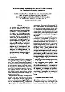
Consider the problem of building a spam detection system. For the matter, we will train a classifier to discriminate between spam and non-spam given a set of features from the email: words contained in the body, subject, sender, meta information, among others. We therefore gather a collection of emails from different users properly labeled as spam or non-spam, to serve as a training data, as shown in Figure 1.1.

Figure 1.1: Collected labeled e-mails from a set of users. In traditional machine learning, two straightforward strategies to built such system are: (i) train a single classifier pooling data from all users (pooling) or (ii) train a classifier for each user using only its data (individual ). Figure 1.2 illustrates both strategies. Training a classifier is a task. Therefore, in the first strategy a single larger task is needed to be done, while in the second multiple tasks exist.

Figure 1.2: Pooling (left) and individual (right) strategies. Clearly, each strategy has its own advantages and limitations. By training a single classifier for all users completely neglects the differences between the users with regard to what is considered spam. The same email may be marked as spam for a user, but not for another. On the other hand, training a classifier for each user in isolation, it allows obtaining a personalized spam detector that will capture particular characteristics of the user. However, as it is trained considering only its own data (emails), the classifier may not be able to detect other possible types of spams or new tricks used by spammers, which may be contained in other user’s emails. Additionally, a new user will have no or very limited amount of labeled emails to train his/her own classifier and, as a consequence, the classifier will perform badly at the beginning. Thus, a strategy that exploits the best of the two worlds is preferable. It is expected that users with similar tastes are very likely to have equivalent classifiers. Assuming it is known that two users agree with what is considered a spam, it is then

20 possible to improve each user’s classifier by exploiting such relationship between users. On the other hand, for completely unrelated users, it might be better to have their classifiers learned in isolation. This general scenario of having multiple tasks that need to be learned simultaneously is also seen in many domains other than spam detection. A similar setting is observed in modeling users’ preferences in a recommendation system; predicting the outcome of a therapy attempt for a patient with certain disease, taking into account his/her genetic factors and the biochemical components of the drugs; multi-label classification with binary relevance transformation, where a classifier for each label is needed to be trained and there should be several related labels. In fact, as will be seen in Chapter 2, even traditional problems that are being modeled as a single task can be posed as multiple task learning.

1.2

Multitask Learning: Exploring Task Commonalities

Multitask learning (MTL) (Caruana, 1993; Baxter, 1997) is a compelling candidate to deal with problems where multiple related models are to be estimated. Multitask learningbased methods seek to improve the generalization capability of a learning task by exploiting commonalities of the tasks. To allow exchange of information, a shared representation is usually employed. Applying the multitask learning idea in the multiple spam filters problem discussed in section 1.1, each user would have its own spam filter, however the training of the classifiers is performed jointly, so that emails from related users are implicitly used. Even though departing from distinct modeling strategies, many multitask learning formulations are in essence instances of a general form, given by: ! nk  m  X 1 X +λ R(θ1 , θ2 , ..., θm ) ` f (xik , θk ), yki minimize | {z } θ1 ,...,θm n (1.1) k i=1 joint regularizer {z } |k=1 joint empirical risk (training error)

where m is the total number of tasks, f is a predictive function, and ` is a loss function. The joint regularizer is responsible for allowing tasks to make use of information from other related tasks, thus improving their own performance. Different hypotheses of how tasks are related lead to distinct characterizations of the joint regularizer. These characterizations and formulations other than the regularization-based on (1.1) exist and are discussed in Chapter 2. Benefits of MTL over traditional independent learning have been supported by many experimental and theoretical works (Evgeniou and Pontil, 2004; Ando et al., 2005; Bickel et al., 2008), (Bakker and Heskes, 2003; Ben-David et al., 2002; Ben-David and Borbely, 2008; Maurer and Pontil, 2013).

1.3

Thesis Agenda: Explicit Task Relationship Modeling

In the large body of research on multitask learning, the assumption that all tasks are related is frequently made. However, it may not hold for some applications. In fact, sharing information with unrelated tasks can be detrimental to the performance of the tasks (Baxter, 2000). Then, a fundamental step is to estimate the true relationship structure among tasks, thus promoting a proper information sharing among related tasks while avoiding using information from unrelated tasks.

21 In this thesis, we investigate the problem of estimating task relationships from the data available and aggregate this information when learning task-specific parameters. The task relationships help to proper control how the data is shared among the tasks. In particular, we propose a family of MTL methods that is built on a hierarchical Bayesian model where task dependencies are explicitly estimated from the data, besides the parameters (weights) of each task. We assume that features across tasks come from a prior distribution. We employ two distributions: a multivariate Gaussian distribution with zero mean and unknown precision (inverse covariance) matrix; and a semiparametric Gaussian copula distribution (Liu et al., 2012) that is known for its flexibility. Thus, task relationship will naturally be captured by the hyper-parameter of the prior distribution. The method is referred to as Multitask Sparse Structure Learning (MSSL). Other variants of the MSSL are also explored in this thesis. Unlike other MTL methods, MSSL measures tasks relationship in terms of partial correlation, which has a meaningful interpretation in terms of conditional independence, instead of ordinary correlation. Experiments in many classification and regression problems from different domains have shown that MSSL significantly reduce the sample complexity, that is, the required number of training samples for the algorithm to successfully learn a target function. Roughly speaking, this is due to the fact that MSSL allows tasks to selectively borrow samples from other related tasks.

1.4

Main Contributions of the Thesis

Our primary contribution in this thesis is to simultaneously learn the structure and the tasks. More specifically we assume that the task relationship can be encoded by an undirected graph. We pose the problem as a convex optimization problem over parameters for each task and a set of parameters which describes the relationship between the tasks. The research developed in the work advances the field of machine learning in the following ways: • We proposed a family of multitask learning models that explicitly estimate and incorporate task relationship structure via a hierarchical Bayesian model. Therefore, besides the set of parameter vectors for all tasks, a graphical representation of the dependence among tasks is estimated. The proposed methods can deal with both classification and regression problems. • Semiparametric Gaussian Copula (SGC) (or nonparanormal) distribution is used as prior for features across multiple tasks in the hierarchical Bayesian model. SGC are flexible models that relaxes the Gaussian assumption of the marginals and their linear correlation, allowing to capture rank-based nonlinear correlation among tasks. To the best of our knowledge, this is the first work that uses Copula models to capture task relationship. • We propose a multilabel classification method based on multitask learning with label dependence estimation. The method consists of two steps: (1) learn the label dependence via Ising-Markov random field; and (2) incorporate the learned dependence in a regularized multitask learning formulation that allows binary classifiers to transfer information during training. • We shed a light on the important problem in climate science called Earth System Model (ESM) ensemble from a multitask learning perspective. Extensive set of experiments were

22 conducted and showed that MTL methods can, in fact, improve the quality of mediumand long-term predictions of temperature and precipitation, which may help to predict climate phenomena such as El-Ni˜ no/La-Ni˜ na. • A hierarchical multitask learning formulation is proposed for the problem of ESM ensemble for multiple climate variables. Here, each task is in fact a multitask learning problem. Two levels of sharing exist: task parameters and task dependencies. A common theme in all of our algorithms is that they are capable of performing a selective information sharing. The guidance is defined by an undirected graph that encodes task relationship and is estimated during the joint learning process of all tasks.

1.5

Thesis Roadmap

The thesis is organized in two major parts: background and the proposals, which we referred to as Multitask with Sparse and Structural Learning. In the background part, Chapters 2 and 3 provide the knowledge, concepts, and tools to support all the proposed models and methods developed in this thesis. We set up the multitask learning problem and discuss the main methods already proposed for the problem. Fundamental tools for dependence modeling are discussed. The second part comprises Chapter 4, 5, and 6 where the main contributions are presented. We may say that the methods proposed in Chapters 5 and 6 are extensions of the formulation presented in Chapter 4. Several portions of this thesis are mainly based on joint works with collaborators. • Chapter 2 formally introduces the multitask learning paradigm. We present an extensive literature review and discuss the methods more related to those proposed in this thesis. Additionally, we compare the multitask learning setting with many related areas in the machine learning community, such as transfer learning, multiple output regression, multilabel classification, domain adaptation, and covariate shift. • Chapter 3 discusses tools to model dependence among random variables with emphasis in the undirected graphical models. The two most common undirected graphical models are presented, namely Gaussian graphical model (or Gauss-Markov Random Field) and Ising models (or Ising-Markov random field). Recent advances in structure learning in those models are also presented. • Chapter 4 introduces our general framework for multitask learning, named Multitask Sparse Structure Learning (MSSL). An extension that uses semiparametric copula models is also proposed. Such model has been recognized for its flexibility to deal with nonGaussian distributions as well as for being more robust to outliers. Parameter estimation aspects of three instances of the MSSL framework are discussed in more details. We apply the proposed method both in classification and regression problems, with emphasis on the problem of Earth System Model ensemble. This chapter is based on Gon¸calves et al. (2014) and Gon¸calves et al. (2015). • Chapter 5 presents a multitask learning method for the problem of multilabel classification, where labels dependence is modeled by an Ising model. The algorithm is referred to as Ising-Multitask Structure Learning (I-MTSL). The effectiveness of the algorithm is

23 demonstrated on several multilabel classification datasets and compared to the performance of well-established methods for the problem. This chapter is based on Gon¸calves et al. (2015). • Chapter 6 extends the MSSL to a hierarchical formulation, referred to as U-MSSL, for multiple ESMs ensemble problem. Compared to MSSL and existing MTL methods that only allow sharing model parameters, U-MSSL is a hierarchical MTL with two levels of information sharing: (1) model parameters (coefficients of linear regression) are shared within the same super-task; and (2) precision matrices, modeling the relationship of subtasks, are shared among the super-tasks by means of group lasso penalty. The conclusions and future directions are provided in Chapter 7.

Part I Background

25

Chapter

2

Overview of Multitask Learning Models

“

The sciences do not try to explain, they hardly even try to interpret, they mainly make models. By a model is meant a mathematical construct which, with the addition of certain verbal interpretations, describes observed phenomena. The justification of such a mathematical construct is solely and precisely that it is expected to work - that is correctly to describe phenomena from a reasonably wide area. Furthermore, it must satisfy certain esthetic criteria - that is, in relation to how much it describes, it must be rather simple.

”

John Von Neumann In this chapter we formally introduce multitask learning (MTL) and present an overview of the existing methods, highlighting their assumptions regarding two key components, task relatedness and shared information. This review will help to properly place our methods in the field. We will also discuss advances in the theory behind multitask learning and how MTL compares to related areas such as multilabel classification, multiple-output regression, transfer learning, covariate shift, and domain adaptation. We discuss the relation between multitask learning and a well-known result in statistics, the Stein’s paradox. The broad spectrum of problems to which multitask learning methods have successfully been applied is also presented.

2.1

Multitask Learning

Learning for multiple tasks, such as regression and classification, simultaneously arise in many practical situations, ranging from object detection in computer vision, going through web image and video search (Wang et al., 2009), and achieving multiple microarray data set integration in computational biology (Kim and Xing, 2010; Widmer and R¨atsch, 2012). The steadily growth of interest in personalized machine learning models, where a model is trained for each entity (such as user or language) also boosts the need of methods to deal with multiple tasks simultaneously. The tabula rasa approach in machine learning is to train a model for each task in isolation, then only looking to its own data. Clearly, the tabula rasa, also known as single task learning, ignores the information regarding the relationship of the tasks. Multitask learning are, therefore, machine learning

26 techniques endowed with a shared representation capacity to allow such relatedness information to flow among the tasks aiming to produce more accurate individual models. As stated by Caruana (1997), “Multitask Learning is an approach to inductive transfer that improves learning for one task by using the information contained in the training signals of other related tasks”. Figure 2.1 shows the conceptual difference between multitask learning and the traditional single task learning. Still a model for each task is considered, but the training of the models is performed jointly to exploit possible relation among them.

Figure 2.1: Difference between multitask learning and traditional single task learning. In MTL the learning process involves all the tasks and is performed jointly, allowing the exchange of information.

2.1.1

General Formulation of Multitask Learning

Multitask learning can be more formally presented as follows. Suppose we are given a set of m supervised learning tasks, such that all data for the k-th task, (Xk ,yk ), come from the space X × Y, where X ⊂ Rd and Y is dependent on the task, for example, Y ⊂ R for regression and Y ⊂ {0, 1} for binary classification. For each task k only a set of nk data samples is available, xik ∈ X and yki ∈ Y, i = 1, ..., nk . The goal is to learn m parameter vectors θ1 , ..., θm ∈ Rd such that f (xik , θk ) ≈ yki , k = 1, ..., m, and i = 1, ..., nk . We denote by Θ a matrix whose column vectors are the parameter vectors, Θ = [θ1 , ..., θm ]. In the learning problem associated with the task k, an unknown joint probability distribution relates the input-output variables, p(Xk , yk ), meaning the probability of observing the input-output pair (xik ,yki ). The parameter vector θ maps the input x to the output y and a loss function ` defined in R2 penalizes inaccuracy of predictions, which includes squared, logistic, and hinge loss as examples. The expected loss, or risk, of the parameter vector θk of the k-th task is E(Xk ,yk )∼p [`(f (Xk , θk ), yk )]. So, in multitask learning we are interested in

27 minimizing the total risk R(Θ) =

m X

E(Xk ,yk )∼p [`(f (θk , Xk ), yk )] =

k=1

m Z X k=1

  ` f (xk , θk ), yk dp(xk , yk ).

(2.1)

X ×Y

As in practice the distribution p is unknown and only a finite set of nk i.i.d. samples Dk = k drawn from such distribution is available, an intuitive learning strategy is the {(xik , yki )}ni=1 ¯ = (D1 , ..., Dm ), empirical risk minimization. With the entire multi-sample represented as D the total empirical risk is computed as follows ! nk  m  X X 1 ˆ ¯ = . (2.2) R(Θ, D) ` f (xik , θk ), yki n k i=1 k=1 However, directly minimizing the total empirical loss is equivalent to solving each task independently nk   1 X k i i θk (D ) = arg min ` f (xk , θk ), yk . (2.3) θk nk i=1 To allow information sharing, a commonly used strategy is to constraint the parameter vectors θk to lie in a (or many) shared unknown subspace(s) B ⊆ Rd , but assumed to have a certain topology that implies mutual dependence among the vectors θk . This is enforced by a regularization on the total empirical risk. As will be seen in the next sections, different assumptions on the dependence among tasks lead to specific forms of regularization. MTL methods in this class are known as regularized multitask learning. Regularized Multitask Learning In the class of regularized multitask learning, the existing methods can be seen as instances of the regularized total empirical risk formulation as follows: ! nk  m  X X 1 ˆ reg (Θ, D) ¯ = ` f (xik , θk ), yki + R(Θ) (2.4) R n k i=1 k=1 where R(Θ) is a regularization function of Θ designed to allow information sharing among tasks. In the next section, we present a survey of the multitask learning algorithms and discuss the regularization functions used to encourage structural task relatedness and how this relates to two important aspects of multitask learning formulations: (i) task relationship assumption, and (ii) types of information shared among related tasks.

2.2

Models for Multitask Learning

MTL has attracted a great deal of attention in the past few years and consequently many algorithms have been proposed (Evgeniou and Pontil, 2004; Argyriou et al., 2007; Xue et al., 2007b; Jacob et al., 2008; Bonilla et al., 2007; Obozinski et al., 2010; Zhang and Yeung, 2010; Yang et al., 2013; Gon¸calves et al., 2014). Therefore, it becomes a great challenge to cover them all. In this chapter, we present a general view of major lines of research in the field, highlighting the most important methods and discussing in more details those more related to the methods proposed in this thesis.

28 Early stages of multitask learning (Caruana, 1993), (Caruana, 1997), and (Baxter, 1997) focused on information sharing in neural network models, particularly hidden neurons. Examples of these formulations will be discussed in the next sections. Lately, most of the proposed methods are formulations belonging to the class of regularized multitask learning (2.4). The existing algorithms basically differ the way the regularization function R(Θ) is designed, including restrictions imposed on the structure of the matrix of parameters Θ and the relationship among tasks. Some methods assume a fixed structure a priori, while others try to estimate such information from the available data. In the next sections, we will present an overview of the MTL methods, categorizing them according to their assumption regarding task relatedness and the information shared.

2.2.1

Task Relatedness

A key component in MTL is the notion of task relatedness. As pointed out by Caruana (1997) and also corroborated by Baxter (2000), it is fundamental that information sharing is allowed only among related tasks. Exchanging information with unrelated tasks, on the other hand, may be detrimental. This is known as negative transfer. It is therefore important to build multitask learning models that benefit related tasks and do not hurt performance of unrelated ones. Some existing multitask learning methods simply assume that all tasks are related and only controls what is shared. Others assume beforehand the task dependence structure, for example in clusters or encoded in a graph, and, therefore, the sharing is determined by such a priori structure. More recently, flexible methods do not assume any dependence beforehand, but learn it from the data jointly with task parameters. From this perspective, we identify three categories of multitask learning methods according to their task relatedness assumption: 1) all tasks are related; 2) tasks are organized in clusters or in a tree/graph structure; and 3) task dependence is estimated from the data. Figure 2.2 presents instances of methods belonging to each of these categories. Task relatedness in Multitask Learning

All tasks are related

Cluster/graph relationship

Dependence learning

Ando et al. (2005)

Evgeniou et al. (2005a)

Zhang and Schneider (2010)

Argyriou et al. (2007)

Xue et al. (2007b)

Rothman et al. (2010)

Jalali et al. (2010)

Bakker and Heskes (2003)

Zhang and Yeung (2010)

Obozinski et al. (2010)

Xue et al. (2007a)

Sohn and Kim (2012)

Chen et al. (2012)

Zhou et al. (2011a)

Yang et al. (2013)

...

...

...

Figure 2.2: MTL instances categorization with regard to task relatedness assumption.

29 All Tasks are Related The assumption of all tasks are related and the information about tasks are selectively shared has been widely explored by multitask learning. Several hypotheses have been suggested on the true structure of the parameter matrix Θ that controls how the information is shared. Table 2.1 presents examples of these assumptions together with the corresponding regularization term R(Θ) deliberately designed to enforce the hypothesized structure.

Mean Regularized

Regularization −R(Θ) Pm P 1 λ1 m t=1 θt k k=1 kθk − m

Joint Feature Selection

λ1 kΘk1,2

(Argyriou et al., 2007)

Dirty Model

λ1 kP k1,∞ + λ2 kQk1

(Jalali et al., 2010)

Low Rank

λ1 kΘk∗

(Ji and Ye, 2009)

Name

Reference (Evgeniou and Pontil, 2004)

λ1 kP k1 Sparse+Low Rank

s.t. Θ = P + Q,

(Chen et al., 2012)

kQk∗ ≤ τ. λ1 η(1 + η)tr(Θ(ηId + M )−1 Θ> ) Relaxed ASO

s.t. tr(M ) = # of clusters M  Id ∈ S+d η=

Robust Feature Learning Multi-stage Feature Learning Tree-guided Group Lasso MTL Sparse Overlapping Sets Lasso MTL

λ2 λ1

λ1 kP k∗ + λ2 kQk1,2

Robust MTL

s.t. Θ = P + Q λ1 kP k2,1 + λ2 kQk1,2 s.t. Θ = P + Q P λ1 dj=1 min(kθi k1 , ξ) PP j λ ωv kθG k v 2 j v∈V

infW

P

(αG kωG k2 + kωk1 ) P ωG = vec(Θ)

G∈G

s.t.

(Chen et al., 2009)

(Chen et al., 2011) (Gong et al., 2012a) (Gong et al., 2012b) (Kim and Xing, 2010) (Rao et al., 2013)

G∈G

Table 2.1: Example of task relatedness assumptions in existing multitask learning models and the corresponding regularizers. Adapted from MALSAR manual (Zhou et al., 2011b). In Thrun and O’Sullivan (1995, 1996) the task clustering (TC) algorithm is proposed to deal with multiple learning tasks. Related tasks are grouped into clusters, where relatedness is defined as the mutual performance gain, whenever a task k improves by knowledge transfer from task k 0 , and vice versa. If it is not the case, tasks are set to different clusters. As a new task arrives, the most related task cluster is identified and only knowledge from this single cluster is transferred to the new task. Evgeniou and Pontil (2004) assumed all tasks are related in a way that the model

30 parameters are close to some mean model. Motived by sparsity inducing property of the `1 norm (Tibshirani, 1996), the idea of structured sparsity has been widely explored in MTL algorithms. Argyriou et al. (2007) assumed that there exists a subset of features that is shared for all the tasks and imposed an `2,1 -norm penalization on the matrix Θ to select such set of features. In the dirty-model proposed in Jalali et al. (2010), the matrix Θ is modeled as the sum of a group sparse and an element-wise sparse matrix. The sparsity pattern is imposed by `q and `1 -norm regularizations. Similar decomposition was assumed in Chen et al. (2012), but here Θ is a sum of an element-wise sparse (`1 ) and a low-rank (nuclear norm) matrix. The assumption that a low-dimensional subspace is shared by all tasks is explored in Ando et al. (2005), Chen et al. (2009), and Obozinski et al. (2010). For example, in Obozinski et al. (2010) a trace norm regularization on Θ is used to select the common low-dimensional subspace. Tasks are Related in a Cluster or Graph Structure Another explored assumption about task relatedness is that not all tasks are related, but instead the relatedness is in a group (cluster) structure, that is, mutual related tasks are in the same cluster, while unrelated tasks belong to different groups. Information is shared only with those tasks belonging to the same cluster. The problem then becomes estimating the number of clusters and the matrix encoding the assignment cluster information. In Bakker and Heskes (2003) task clustering is enforced by considering a mixture of Gaussians as a prior over task parameters. Evgeniou et al. (2005b) proposed a task clustering regularization to encode cluster information in the MTL formulation. Xue et al. (2007b) employs a Dirichlet process (DP) prior over the task coefficients to encourage task clustering, with the number of clusters being automatically determined by the prior. DP prior allows to cluster the coefficients for all features in the same manner, and therefore it does not afford the flexibility to allow feature-dependent task clustering. To mitigate such restriction, a more flexible clustering formulation is presented in Xue et al. (2007a), a matrix stick-breaking process prior to encourage local clustering of tasks with respect to a subset of the features. Table 2.2 shows instances of regularization functions R(Θ) used to encourage task clustering. Name

Regularization −R(Θ)

Reference

Graph Structure

λ1 kΘRk2F + λ2 kΘk1 Pt > 2 i=1 kΘXi − M Pi kF

(Li and Li, 2008)

Multitask Clustering Clustered MTL Clustering

α(tr(Θ> Θ) − tr(F > Θ> ΘF )) + βtr(Θ> Θ)

(Gu and Zhou, 2009) (Zhou et al., 2011a)

Table 2.2: Instances of MTL formulations with the cluster task relatedness assumption. Adapted from MALSAR manual (Zhou et al., 2011b). For graph structured MTL approaches, two tasks are related if they are connected in a graph, i.e. the connected tasks are similar. The similarity of two related tasks can be represented by the weight of the connecting edge (Kim and Xing, 2010; Zhou et al., 2011a). The absence of connection between two nodes in the graph indicates that the corresponding tasks are unrelated and, consequently, no information is shared. Actually, many of the formulations associated with the dependence learning category that will be presented next, boils down to represent the task relationships by means of a graph that is explicitly learned from the training data.

31 Explicitly Learning Task Dependence Forcing transfer learn between tasks which are not related may hurt the performance of learning, a situation which is often referred to as negative transfer (Pan and Yang, 2010). So, it is crucial to properly identify the true structure among tasks. Recently, there have been some proposals to estimate and incorporate the dependence among the tasks into the learning process. The majority of them resort to hierarchical Bayesian models, more specifically assuming some prior distribution over the task parameter matrix Θ that captures task dependence information. Figure 2.3 depicts the arrangement of a regular hierarchical Bayesian model. Data for each task is assumed to be sampled from a parametric distribution defined by its parameter θk , which in turn are samples of a common prior distribution p(π) which may carry information from the dependence of the vectors of parameters θk , k = 1, ..., m.

Figure 2.3: Graphical representation of a hierarchical Bayesian model for multitask learning. Tasks parameter vectors θk , k = 1, ..., m are independent samples from the same prior distribution p(π). A matrix-variate normal distribution was used as a prior for Θ matrix in Zhang and Yeung (2010). The hyper-parameter for such a prior distribution captures the covariance matrix among all task coefficients. The resulting non-convex maximum a posteriori problem is relaxed by restricting the model complexity. It has a positive side of making the whole problem convex, but has the downside of significantly restricting the flexibility of the task relatedness structure. Also, in Zhang and Yeung (2010), the task relationship is modeled by the covariance among tasks, but uses the inverse in the task parameter learning step. Therefore, the inverse of the covariance matrix have to be computed at every iteration. Zhang and Schneider (2010) also used a matrix-variate normal prior over Θ. The two matrix hyper-parameters explicitly represent the covariance among the features (assuming the same feature relationships in all tasks) and covariance among the tasks, respectively. Sparse inducing penalization on the inverse of both is added into the formulation. Unlike Zhang and Yeung (2010), both matrices are learned in an alternating minimization algorithm and can be computationally prohibitive in high dimensional problems due to the cost of modeling and estimating the feature covariance. Yang et al. (2013) also assumed a matrix-variate normal prior for Θ. However, the row and column covariance hyperparameters have a Matrix Generalized Inverse Gaussian (MGIG) prior distribution. The mean of matrix Θ is factorized as the product of two matrices that also has matrix-variate normal distribution as a prior. The model inference is done via a variational Expectation Maximization (EM) algorithm. Due to the lack of a closed form expression to compute statistics of the MGIG distribution, the method resort to sampling techniques, which can be slow for high-dimensional problems.

32 Unlike most of the aforementioned methods that model task correlation by means of the task parameters, in the multivariate regression with covariance estimation (MRCE) presented in Rothman et al. (2010), the correlation of the response variables arises from the correlation in the errors, that is, the i.i.d. residuals 1 , 2 , ..., n ∼ Nm (0, Ω). Therefore, two tasks are related if their residuals are correlated. Sparsity on both Θ and Ω is enforced. Rai et al. (2012) extended the formulation in Rothman et al. (2010) to model feature dependence, additionally to the task dependence modeling. However, it is computationally prohibitive for high-dimensional problems, due to the cost of estimating another precision matrix for feature dependence. Zhou and Tao (2014) used copula as a richer class of conditional marginal distributions p(yk |x). As copula models express the joint distribution p(y|x) from the set of marginal distributions, this formulation allows marginals to have arbitrary continuous distributions. Output correlation is exploited via the sparse inverse covariance in the copula function, which is estimated by a procedure based on proximal algorithms. Our method also covers a rich class of conditional distributions, the exponential family that includes Gaussian, Bernoulli, Multinomial, Poisson, and Dirichlet, among others. We use Gaussian copula models to capture tasks dependence, instead of explicitly modeling marginal distributions. All the methods proposed in this thesis lie in this category. Task relationship structure will be explicitly captured by a hyper-parameter of a prior distribution in a hierarchical Bayesian model. We learn such a structure given that it is not available beforehand. As it will be discussed in Chapters 4, 5, and 6, the task relationship representation will, in fact, be given by an undirected graph with nice properties such as conditional dependence among tasks.

2.2.2

Shared Information

As discussed earlier, the central issue in multitask learning is to share information between related tasks. A follow-up question is what do related tasks share? Or, more precisely, what kind of information two related tasks share to each other? Researchers answered this question in different manners. Considering the type of information shared, the existing multitask learning algorithms can be mainly categorized into four lines of research: (i) data samples, (ii) model parameters or prior, (iii) features, and (iv) nodes of neural networks. Figure 2.4 presents few examples of existing MTL approaches in each of the four mentioned assumption. The assumption of data samples sharing has not been explored in much of the existing MTL formulations. In fact, few methods followed this direction. It is probably due to the need of modeling joint distributions p(X, Y ) for all tasks, which for high-dimensional problems is quite challenging. This is commonly used in domain adaptation and covariate shift methods under the name of importance weighting methods (Jiang and Zhai, 2007). We will present a brief discussion on these two problems, that are closely related to MTL, later in this chapter. In the second category, the formulations assume that related tasks share similar parameter vectors. We may say that most of MTL methods, particularly the regularized ones, fall in this category. Many others assume that task parameter vectors are samples drawn from a common prior distribution, in a hierarchical Bayesian modeling. The majority of the methods that perform task dependence learning fall in this category. Methods in the last category assume that if tasks are related they should share a common feature space. The goal is then to learn a low-dimensional representation shared across related tasks. The full set of features of a certain task is usually the combination of a subset of

33 Shared information in Multitask Learning

Data samples

Model parameters or prior

Features

Nodes of Neural Networks

Bickel et al. (2008)

Bakker and Heskes (2003)

Ando et al. (2005)

Caruana (1993)

Bonilla et al. (2007)

Evgeniou and Pontil (2004)

Evgeniou and Pontil (2007)

Caruana (1997)

Quionero-Candela et al. (2009)

Xue et al. (2007b)

Ji et al. (2008)

Collobert and Weston (2008)

...

Li and Li (2008)

Liu et al. (2010)

Seltzer and Droppo (2013)

Agarwall et al. (2010)

Luo et al. (2013)

Zhang et al. (2014)

Zhang and Yeung (2010)

...

Setiawan et al. (2015)

...

Figure 2.4: Lines of research regarding the information shared among related tasks. features shared with all the related tasks and a subset of task specific features. Multitask learning has been used with neural networks in two distinct ages of the MTL development: at the very beginning with the seminal works of Caruana (1993) and Caruana (1997), and recently with the renewed interest in neural networks due to the rising of the deep neural networks, with particular application in natural language processing (Collobert and Weston, 2008), computer vision (Seltzer and Droppo, 2013), and machine translation (Zhang et al., 2014). These areas have seen significant progress with the combination of deep neural networks and multitask learning.

2.2.3

Placing Our Work in the Context of MTL

In this thesis, we propose a family of MTL methods capable of estimating task dependence from the data and incorporating this information in the learning process of task parameters. To do so, the joint learning is allowed via a hierarchical Bayesian model, where we assume that features of all tasks have a common prior distribution, where the hyper-parameter of such distribution encodes task dependence. Two classes of prior distributions are proposed in this work. First, a multivariate Gaussian distribution is assumed. As will be clear in the next chapters, it implies that task parameters for each task is normally distributed with zero mean and unknown standard deviation, besides that the tasks are linearly correlated through the precision matrix of the Gaussian prior (hyper-parameter). Second, a flexible copula distribution is assumed. It implies a much weaker assumption of the individual task parameter distribution, which can now be any parametric or even non-parametric distribution, and task parameters can be non-linear correlated. Therefore, we may say that the methods developed in Chapters 4, 5, and 6 belong to the category of methods with dependence learning, with regard to the task relatedness assumption, and to the category of model parameters or prior, in respect to the kind of information shared among related tasks. The advantages and limitations of the methods presented in this thesis when compared to the existing ones will be discussed throughout the corresponding

34 chapters.

2.3

Theoretical Results on MTL

Theoretical investigations have been carried out to clearly expose the conditions under which multitask learning is preferable to single task learning. Bounds were given for general multitask learning problems as well as for formulations with special assumptions of task relatedness Ben-David and Schuller (2003); Maurer and Pontil (2013) (including some of those in Table 2.1). These bounds provide a quantitative measure of how much MTL methods can improve single task learning with regard to characteristics of the problems, such as the distributions underlying the training data. In a seminal work on theoretical analysis of multitask learning, Baxter (2000) used covering numbers to derive general (uniform) bounds on the average error of m related tasks. From the results, Baxter claims that “learning multiple related tasks reduces the sampling burden required for good generalization, at least on a number-of-examples-required-per-task basis”. In other words, multitask learning requires a smaller number of training samples per task when compared to single task learning to achieve the same level of generalization capability. Closely related to Baxter (2000), Ando et al. (2005) also provided generalization bounds using Rademacher averages and a slightly different definition of covering numbers. The provided bounds show that by minimizing the joint empirical risk in (2.2) instead of independent empirical risk of each task, it is possible to estimate the shared subspace more reliably as the number of tasks grows (m → ∞). Lounici et al. (2011) provided bounds for a multitask learning formulation with the assumption that tasks share a small subset of features, induced by Group Lasso penalty. The bounds show that Group Lasso regularization is more advantageous than the usual Lasso in the multitask setting. More precisely, MTL with Group Lasso regularization achieves faster rates of convergence in some cases as compared to MTL with Lasso penalty. Maurer and Pontil (2013) used the method of Rademacher averages and results on tail bounds for sum of random matrices to establish excess risk bounds for a multitask learning formulation with trace norm regularization (tasks share a common low dimensional space) with explicit dependence on the number of task, number of examples per task and properties of data distribution. Excess risk measures the difference between the total empirical risk in (2.2) and the theoretical optimal one given by (2.1). From the derived bounds, it is possible to say that MTL with shared low rank subspace has a worse bound than standard bounds for single task learning if the mixture of data distribution from all tasks are supported on a very low dimensional space. In other words, when the problem is already easy, the bounds for the MTL formulation with low rank regularization show no benefit.

2.4

Stein’s Paradox and Multitask Learning

We have shown so far that multitask learning is grounded on the principle that jointly learning multiple related tasks and therefore allowing to exploit possible commonalities can improve performance of individual tasks. A well known result in statistics due to Stein (1956) corroborates which such hypothesis, the Stein’s paradox. It states that when three or more parameters are estimated simultaneously, there exist combined estimators more accurate on average (that is, having lower expected mean squared error) than any method that estimates the parameters separately.

35 The Stein’s paradox can be state more formally as follows. Let X = X1 , ..., Xm be a set of independent normally distributed random variables, i.e., Xk ∼ N (µ, 1) for k = 1, ..., m. We are interested in finding an estimator for the unknown means µ1 , ..., µm . Let us consider mean squared error as measure of the quality of our estimation Z  2 2 ˆ }= ˆ Rµˆ (µ) = E{kµ − µk µ(x) − µ p(x|µ)dx. (2.5) In other words, the risk function measures the expected value of the estimator’s error (the loss ˆ is admissible if there is no other estimator µ∗ with function). We say that an estimator µ ˆ is admissible for m ≤ 2, smaller risk, that is, Rµ∗ (µ) ≤ Rµˆ (µ) for all µ. Stein proved that µ but inadmissible for m ≥ 3. And in James and Stein (1961) the authors proposed an estimator, which lately became the James-Stein (JS) estimator, that strictly dominates the traditional maximum likelihood estimator for m ≥ 3, that is, the JS estimator always achieves lower MSE than the maximum likelihood estimation:   m−2 JS ˆ (X) = 1 − X. (2.6) µ kXk2 Most surprisingly is that no matter if variables Xk are candy weights, price of banana, and the temperature in Rio de Janeiro in Summer, Stein showed that it is better, in a mean squared error sense, to jointly estimate the means of m Gaussian random variables using data sampled from all of them, even if they are independent and have different means. So, it is beneficial to consider samples from seemingly unrelated distributions in the estimation of the t-th mean. The Stein’s paradox can be seen as an early evidence of the soundness of multitask learning hypothesis, although counterintuitive as it works even for completely unrelated random variables. MTL on the other hand focus on sharing information among related tasks while avoiding sharing with unrelated ones. Also, MTL seeks to estimate fairly general task parameters with unknown distribution, rather than means of Gaussian distributed variables as in the Stein’s paradox.

2.5

Multitask Learning and Related Areas

Within the machine learning community there are areas closely related to multitask learning. In the next sections, we will discuss the similarities and differences among those areas, which include multiple-output regression, multilabel classification, transfer learning, domain adaptation and covariate shift. This will help to clarify the overlapping between the areas and identify if and when multitask learning methods can be applied to the problems arising from those areas.

2.5.1

Multiple-Output Regression

The problem of multiple-output regression (or multivariate response prediction) has been studied in the statistics literature for a long time. Unlike classical regression that aims to predict a single response given a set of covariates, in multiple-output regression we seek to estimate a mapping function from a multivariate input space X ⊂ Rd to a multivariate output space Y ⊂ Rm , that is, estimate a function f : X → Y. Let us consider the multiple-output

36 linear regression model. Given a set of samples {(xi , yi )}ni=1 ⊂ X × Y, the linear regression model is defined as yi = Θ> xi + i , ∀i = 1, ..., n. (2.7) where i ∼ N (0, σ 2 ) is the residual, and Θ = [θ1 , ..., θm ] is an d × m weight matrix whose columns are the weights for each output. The maximum likelihood cost function is written as n m X 1X i J(Θ) = (yk − θk> xi )2 . n i=1 k=1

(2.8)

Comparing (2.8) with the MTL formulation in (2.4) two important differences stand out: (i) there are m independent single response regression problems, no regularization added; and (ii) the inputs (covariates) are the same for all regressors, that is, X1 = X2 = ... = Xm . Hence, classical multi-output regression problem can be seen as a specific case of multitask learning problem, where no information is shared among tasks (independent learning) and the input data X is the same for all tasks. As will be seen in Section 2.5.2, the same happens for multilabel learning using binary relevance decomposition. In order to take correlation between outputs into account, many papers have proposed ways of capturing and incorporating output dependence information in the joint estimation problem (Brown and Zidek, 1980; Breiman and Friedman, 1997). In principle, any multitask learning method for regression can be applied in multiple output regression, as they were particularly designed to deal with multiple task problems by exploiting relationship among them. In fact, some recently proposed multiple output regression methods are multitask learning methods (Rothman et al., 2010; Rai et al., 2012; Li et al., 2014).

2.5.2

Multilabel Classification

Similarly to the extension of ordinary single output regression methods to deal with multiple outputs, we may consider multilabel classification as an extension to the single label classification problems. In multilabel classification a single data sample x is associated with m > 2 labels. For example, an image possibly contains a set of elements such as trees, cars, people and streets. Then, given a new image we want to check which of these elements are present. More formally, let X ⊂ Rd and Y ⊂ {0, 1}m be the input and output space, respectively. Given a training set {(xk , yk )}m k=1 ⊂ X × Y, we seek to estimate a classifier function f : X → Y that generalizes well beyond the training samples. One of the most common approaches to deal with multilabel classification is through problem transformation. It transforms the multilabel classification problem in conventional classification problems such as binary and multi-class, so that we can use off-the-shelf classifiers (Tsoumakas and Katakis, 2007). In the binary relevance transformation, the multilabel classification problem split in m independent binary classifiers and a classifier is then trained independently for each label. Clearly, it has the same characteristics as multiple-output regression: ignores labels (tasks) dependence and the input data are the same for all tasks. Likewise, we can see multilabel classification with binary relevance transformation as a specific case of MTL. Naturally, many papers proposed methods that take relationship among the classifiers into account (Rai and Daume, 2009; Zhang and Zhang, 2010; Read et al., 2011; Marchand et al., 2014). Considering the fuzzy boundaries between multilabel classification with binary relevance transformation and multitask learning, it was expected that proposed methods for multilabel classification are in fact multitask learning method (Luo et al., 2013).

37 In this thesis we propose a multilabel classification method based on multitask learning that explicitly models label dependence through an Ising-Markov random field. This new formulation is discussed in Chapter 5.

2.5.3

Transfer learning

In transfer learning, one seeks to leverage knowledge obtained in a previous source task, to a new related learning target task. To more formally pose the transfer learning problem, we need to introduce the concepts of domain and task. A domain D consists of two elements: the input or feature space X and the marginal probability distribution p(X), where X ⊂ X . Then, D = {X , p(X)}. A task T also consists of two elements, the output or label space Y and a predictive function f , which is also represented as the conditional probability p(Y |X) with Y ⊂ Y. Then, T = {Y, p(Y |X)}. In most practical cases, the number of source domain data nS is much larger than the target domain, nT , that is, 0 ≤ nT  nS . The question regarding the availability of labels in the source and target domains will lead to a discussion that is out of the scope of this section. For a comprehensive exposition of this topic, we refer interested readers to Pan and Yang (2010). Here, we assume that both source and target contain labeled data, but as just mentioned 0 ≤ nT  nS . In the following, we reproduce the formal definition of transfer learning due to Pan and Yang (2010) that will serve as the basis for our discussion. From this definition we will be able to present two closely related areas, domain adaptation and covariate shift, as specific settings of transfer learning. Definition 2.5.1 (Transfer Learning) Given a source domain DS and learning task TS , a target domain DT and learning task TT , transfer learning aims to help improve the learning of the target predictive function fT in DT using the knowledge in DS and TS , where DS 6= DT or TS 6= TT . From the above definition, we notice three distinctive characteristics from the multitask learning setting: (i) it contains only two tasks - source and target; (ii) we care most about the target task; and (iii) the transfer is sequential (usually the source task is learned, then the target). The aim is to improve performance of the target task, while in multitask learning the goal is to improve the performance of all tasks, no preference is enforced. In transfer learning, source task is more like an secondary information provider. Other aspect is that MTL involves parallel transfer while transfer learning is built on sequential transfer. Figure 2.5 shows a comparison between transfer and multitask learning in terms of how the information is shared among tasks. In transfer learning the information flows asymmetrically from source to target task, while in multitask learning the information is, in principle, allowed to flow symmetrically among the tasks. Due to this perspective, transfer learning is sometimes referred to as asymmetric multitask learning (Xue et al., 2007b). In fact, there is also a more general setting of transfer learning where multi-source domains exist. The problem is to transfer knowledge acquired from multiple source domains to a target domain (Luo et al., 2008), but here we focus on the standard transfer learning setting with two domains, which is the most common in practice. The premise in transfer learning is that the source and target domains are related but not the same. The tasks can differ in two aspects: the domain, DS 6= DT , or the learning tasks, TS 6= TT . Except for specific problems, in practice we have a little understanding on how the source and target differ. Therefore, assumptions on the mismatch are made. Depending on the assumption, the resulting problem has already been studied before under different names including domain adaptation (Ben-David et al., 2007; Daume, 2007) and covariate shift (Shimodaira, 2000).

38

Transfer Learning

Source Task

Multitask Learning Task 1

Task 3

Task 2

Task 4

Target Task

Figure 2.5: In transfer learning the information flows in one direction only, from the source task to the target task. In multitask learning, information can flow freely among all tasks. Adapted from Torrey and Shavlik (2009). Domain Adaptation In domain adaptation, the problem is to learn the same task but in different domains. The idea is to leverage information from the source joint distribution pS (X, Y ) to help model the distribution of the target domain pT (X, Y ). As the joint distribution can be decomposed as p(X, Y ) = p(Y |X)p(X), the source and target domain can differ from one of the two factors: the conditionals where pS (Y |X) deviates from pT (Y |X) to some extent while pS (X) and pT (X) are quite similar; or the marginals where pS (X) deviates from pT (X), but the conditionals are in agreement (Jiang and Zhai, 2007). As will be seen in the next section, the later is equivalent to the problem of covariate shift (Shimodaira, 2000). The domain adaptation problem has received considerable attention in the natural language processing community, as very often one faces the situation where a large collection of labeled data from a source domain is available for training, but we want our model to perform well in a second target domain, for which very little data is available (Daume, 2007). Domain adaptation can be considered distinct from multitask learning as it consists of learning the same task but in different domains. It can, however, be treated as a special case of multitask learning, where we have two tasks, one on each domain, and the class label sets of these two tasks are the same. Without any change, existing multitask learning methods can readily be applied if labeled data from the target domain is available. Some recently proposed domain adaptation are essentially multitask learning algorithms. In Daume (2007) a simple method for domain adaptation based on feature expansion in proposed. The idea is to make a domain-specific copy of the original features for each domain. An instance from the k-th domain is then represented by both the original features and the specific features to the k-th domain. It can be shown that when linear classification algorithms are used, this feature duplication based method is equivalent to decomposing the model parameter θk for the k-th domain into θc + θk0 , where θc is shared by all domains. This formulation then is very similar to the regularized multitask learning method proposed by Evgeniou and Pontil (2004). Covariate Shift A different assumption about the connection between source and target domain is made in the covariate shift problem. Here, we assume that predictive function or the conditionals remain unchanged in the source and target domain, pS (Y |X) = pT (Y |X), but the distribution of the inputs (covariates) are different, pS (X) 6= pT (X) (Shimodaira, 2000). We

39 1.6

0.8 Input

True function

1.4

0.6

1.2

0.4 Target p(X) →

1 0.8 0.6

0.2

Target

0

Source p(X) →

−0.2

0.4

−0.4

0.2

−0.6

0 −1

Source

0

1

2

−1

3

0

1

2

3

Figure 2.6: [Best viewed in color.] Covariate shift problem. Conditionals in each domain are the same (right) but the marginals, the covariates, are shifted (left). We observe that a linear model estimated on the source data is completely different from a model based on target data, even though the true function (conditional) is the same. can say that covariate shift problem is a specific case of domain adaptation. An illustrative example of covariate shift is shown in Figure 2.6. We observe that the underlying conditional distribution is the same but the marginals are different. In multitask learning we usually do not restrict the distributions of the tasks to be the same, so it can be seen as a less restrictive problem than covariate shift. If we treat the learning tasks of source and target domains as two different tasks, we can directly apply existing multitask learning methods. We must say that the discussed research areas and their overlapping with multitask learning are very often interpreted differently by distinct research groups. Additionally, these terms are sometimes used interchangeably.

Transfer Learning

Domain adaptation

Covariate shift

Multilabel classification

Multiple output regression

Multitask Learning Figure 2.7: Venn diagram showing the overlapping between MTL and some related areas in the machine learning community. Multitask learning methods can mostly be applied in problems from those areas. The main characteristics of each of these related areas can be summarized as follows:

40

• Multitask Learning:

• Transfer Learning:

– Model the task relatedness;

– Define source and target domain;

– Learn all tasks simultaneously;

– Learn on the source domain;

– Tasks may have different data/features.

– Generalize on the target domain.

• Multilabel Classification:

• Multiple output regression:

– Model label dependence;

– Model output dependence;

– Learn all classifiers simultaneously;

– Learn all regressors simultaneously;

– Labels share the same data/features;

– Labels share the same data/features;

• Domain Adaptation:

• Covariate Shift:

– Define source and target domain; – Different pS (X|Y ) 6= pT (X|Y );

conditionals:

– Similar marginals: pS (X) ≈ pT (X);

2.6

– Define source and target domain; – Same conditionals: pS (X|Y ) = pT (X|Y ); – Different marginals: pS (X) 6= pT (X);

Multitask Learning can Hurt

In the initial work of multitask learning, Caruana already identified the possibility of a multitask learning method to degenerate the performance of the learning tasks: “MTL is a source of inductive bias. Some inductive biases help. Some inductive biases hurt. It depends on the problem.” (Caruana, 1997). Later, both theoretical and experimental studies in many domains confirmed his words. Since then, researchers have attempted to identify under which conditions MTL strictly improves performance compared to single task learning. Advances in theoretical studies have helped on this issue. Aligned to what is found in the literature of multitask learning, we have experienced and will discuss in the experimental sections, in Chapters 4, 5, and 6, that MTL methods clearly pay off in situations where the number of samples is relatively small compared to the dimension of the problem. As the number of training samples increases, its performance is equivalent to single task learning. In scenarios where the tasks are completely unrelated, MTL usually does not help, and may even hurt the performance. Methods such as those proposed in this research are less susceptible to performance drop, as the task dependence is automatically identified, based on a measure of relatedness, thus avoiding information sharing among unrelated tasks. On the other extreme case, where all tasks are almost identical, simply performing a single task with data samples combined from all tasks will perform similarly to any MTL method. As a general advice, before applying an MTL method, it is important to investigate the characteristics of the tasks we are dealing with. Domain knowledge usually helps on this matter.

41

2.7

Applications of MTL

The need for learning multiple related models simultaneously arises in many fields of research. Additionally, some traditional machine learning problems were also transformed as multitask learning problems, and then benefiting from the power of MTL methods. Examples are multilabel classification and multiple output regression problems which can be decomposed as a set of binary classification or single output regression problems and then multitask learning methods can be used, such as in Luo et al. (2013) and Rai et al. (2012). Generally speaking, any problem which requires solving multiple related tasks can be tackled with multitask learning methods. In the following, we will present a set of fields that have been successfully applied multitask learning methods. In natural language processing (NLP), Collobert and Weston (2008) proposed a unified convolutional deep neural network architecture that learns features relevant to several NLP tasks including part-of-speech tagging, chunking, named-entity recognition, learning a language model and the task of semantic role-labeling. All tasks are learned jointly in a multitask learning setting. Multitask learning for phoneme recognition was presented in Seltzer and Droppo (2013), where additionally to the classification task a secondary task using a shared representation was trained jointly. Three choices of secondary task were tested: the phone label, the phone context, and the state context. In Bordes et al. (2014), a neural network was used to train a semantic matching energy function via multitask learning across different knowledge sources such as Wordnet, Wikipedia, ConceptNet, among others. The authors applied the model to the problem of open-text semantic parsing. In Bickel et al. (2008), a multitask learning method based on data samples sharing was proposed to the problem of HIV therapy screening. Here, a task is to predict the outcome (success or failure) of a therapy or combination of drugs for a given patient’s treatment history and features of the viral genotype. The multitask learning methods were able to make predictions even for drug combinations with few or no training examples and improved the overall prediction accuracy. Web search ranking problems from different countries was taken as a multitask learning problem in Chapelle et al. (2010). Each task is to learn a country-specific ranking function, then learning various ranking functions jointly for multiple countries improved performance of each country. Web page categorization was also studied under the multitask learning setting in Chen et al. (2009), where the goal is to classify documents into a set of categories and the classification of each category is a task. The tasks of predicting different categories may be related. Computer vision also took part of the advances in multitask learning. Face verification for web image and video search was also posed as a multitask learning problem in Wang et al. (2009). In Zhang et al. (2014), a deep neural network with multitask learning was proposed for facial landmark detection, where the target of landmark detection is jointly learned with a set of auxiliary tasks, including inferences of “pose”, “gender”, “wear glasses”, and “smiling” detection. In fact, the marriage between deep neural network and multitask learning has brought a significant advance is the fields of computer vision and image processing. Multilabel image classification that exploits labels relationship through multitask learning settings were studied in Huang et al. (2013) and Luo et al. (2013). In medicine, multitask learning has been considered in multi-subject fMRI studies (Rao et al., 2013). Functional activity is classified using brain voxels as features. A task is to distinguish, at each point in time, which stimulus of a given subject was processed. Alzheimer’s disease progression modeling was also studied from the multitask learning perspective and a

42 task is seen from different ways. While Zhou et al. (2013) considered the prediction at each time point as a task, Zhang and Shen (2012) looked at different tasks corresponding to prediction of different variables. Multitask learning has also being successfully applied to problems arising from computational biology (Widmer and R¨atsch, 2012) and bioinformatics (Xu and Yang, 2011). In Widmer et al. (2010), a multitask learning based method was proposed to deal with the splicesite prediction problem. Prediction for each organism was taken as a task. The hierarchical structure associated with the taxonomy of the organisms was used as a guide for task information sharing. Learning host-pathogen protein interactions in several diseases was tackled under the multitask learning setting in Kshirsagar et al. (2013). A task in such scenario is the set of host-pathogen protein interactions involved in one disease. In signal processing, researchers have looked at problems with the multitask learning lens. MTL based compressive sensing (CS) framework has been developed (Qi et al., 2008), (Ji et al., 2009), where each CS measurement represents a sensing task. The basic tasks can be posed as a sparse linear regression problem for each signal.

2.8

Chapter Summary

The goal of this chapter was to provide an introduction to multitask learning, a machine learning paradigm which seeks to exploit the relatedness of tasks by learning them jointly. We presented a survey on the existing MTL methods, categorizing them in terms of their assumption on the task relationship and the information shared. Advances in theoretical results in MTL have also been discussed aiming to precisely determine under which conditions MTL methods are preferred. Additionally, we compared the multitask learning with related fields within the machine learning realm. Chapters 2 and 3 are devoted to provide the foundations on which the proposed methods of Chapters 4, 5 and 6 are built on.

43

Chapter

3

Dependence Modeling with Probabilistic Graphical Models

“

The purpose of computation is insight, not numbers.

” Richard Hamming

In this chapter, we review undirected graphical models - also known as Markov Random Fields (MRFs), and explore modern methods for learning the structure of these models in high-dimensions. We will focus on two popular instances of MRFs, namely Gaussian Markov Random field (GMRF) and Ising Markov Random field (IMRF). While GMRF represents a typical continuous MRF, the IMRF is commonly used to represent discrete MRFs. These are simple models that are fully specified by their first two moments and have shown to be rich enough for a wide range of applications. We also discuss an extension of Gaussian graphical models for non-Gaussian data that is based on copula theory. As will be discussed in Chapter 4, the structure of the MRFs will be used as a guide for information sharing between tasks in a multitask learning setting.

3.1

Probabilistic Graphical Models

Probabilistic graphical models (PGMs) provide a unifying framework for capturing complex dependencies among random variables, and building large-scale multivariate statistical models (Wainwright and Jordan, 2008). PGMs bring together graph and probability theory, in which random variables are represented as nodes and edges indicate relationship among variables. Exploiting structural properties of the graph can dramatically reduce the complexity of statistical models as well as provide additional insights into the system under observation, for example, by showing how different parts of the system interact. When the problem involves the study of a large number of interacting variables, graphical models are particularly an appealing tool. Recent advances in structure learning in high-dimensional graphical models have attracted the interest of researchers, mainly for relationship discovery. The main aspect of graphical models is that a collection of probability distributions is factored according to the structure of an underlying graph. Concerning the direction of the edges in the graph, two major families of PGMs are: directed graphical models (DGM)

44

1

2

3

4

1

2

3

5 6

4

5 6

7 (a) Directed graphical model: node 5 is conditionally independent on all other nodes, given its parents 3 and 4.

7 (b) Undirected graphical model: node 5 is conditionally independent on all other nodes, given its neighborhood, nodes 3, 4, 6, and 7.

Figure 3.1: Conditional independence interpretation in directed graphical models (a) and undirected graphical models (b).

(or Bayesian networks) and undirected graphical models (UGM) also called Markov random fields (MRFs). We will use the acronyms MRFs and UGM interchangeably in this chapter. In fact, there is also a less common class of models, known as mixed directed and undirected representation, such as the chain graphs (Lauritzen and Richardson, 2002; Drton, 2009). In DGMs, the joint distribution of m random variables X = (X1 , ..., Xm ) is represented by a directed acyclic graph in which each node k, representing a random variable Xk , receives directed edges from its set of parent nodes pa(Xk ). The probabilistic interpretation from the acyclic graph is that a random variable Xk is conditionally independent on all other variables given the variables corresponding to its parent nodes. UGMs represent the joint distribution of a set of variables by an undirected graph and it is factored as a product of functions over the variables in each maximal clique (fully-connected subgraphs). A random variable Xk is conditionally independent of the random variables that are not connected to Xk (do not belong to its neighborhood). See Figure 3.1 for an example. Details on UGMs are presented in the next section. Due to the absence of edge orientation, MRFs may be more suitable for some domains as image analysis and spatial statistics. MRFs can represent certain dependencies that a directed graphical model (Bayesian network) can not, such as cyclic dependencies, on the other hand, it can not represent asymmetric dependencies, for example. In the last decade, structure learning in MRFs have seen an enormous advance motivated by the need of analyzing high-dimensional data such as fMRI, genomic, and social networks, where usually one is also interested in studying how brain regions, genes, and people are acting together. For discovering the dependence graph from a set of data samples, many efficient algorithms have been proposed. These modern data-intensive methods will be discussed in the next sections. The problem of structure learning in undirected graphical models will appear naturally from the MTL formulations proposed in Chapters 4 and 5. This graph will basically encode the task dependencies structure. For this reason, in this chapter we will present an overview of undirected graphical models.

45

3.2

Undirected Graphical Models

Undirected graphical models, also known as Markov random fields (MRFs), are a powerful class of statistical models that represent distributions over a large number of variables using undirected graphs. The structure of the graph encodes Markov conditional independence assumptions among the variables. MRF is a collection of m-variate distributions p(X) = p(X1 , ..., Xm ), with discrete or continuous state space Xk ∈ X , that factorize over a graph G (Wainwright and Jordan, 2008): p(X) = p(X1 , X2 , ..., Xm ) =

1 Y φc (Xc ) Z c∈C

(3.1)

G

where CG are the set of all maximal cliques P of the Q graph G, i.e., the set of cliques that are not contained within any other clique and Z = x c∈CG φc (Xc ) is a normalization constant. The semantics of the undirected graphical model is that a variable is conditionally independent of all other variables given its neighbors in the graph. From the graph in Figure 3.1, it is possible to say that node 5 is conditionally independent of all other nodes, given its neighborhood, composed of nodes 3, 4, 6 and 7. Based on the connection between conditional independence and the absent of edges in the graph, the problem of assessing conditional independence among random variables belonging to the family of distribution of the form (3.1) reduces to the problem of estimating the structure of the underlying undirected graph. This result is formally stated by the HammersleyClifford theorem. The proof can be found in Besag (1974) and Lauritzen (1996). Theorem 3.2.1 (Hammersley-Clifford) A positive distribution p(X) satisfies the conditional independence properties of an undirected graph G iff p can be represented as a product of factors, one per maximal clique, i.e. 1 Y φc (Xc |ωc ) (3.2) p(X) = Z(ω) c∈C G

where C is the set of all (maximal) cliques of G, and the partition function Z(ω), which ensures the overall distribution sums to 1, is given by XY Z(ω) , φc (Xc |ωc ). (3.3) X c∈CG

In general terms, the theorem states that any positive distribution whose conditional independence properties can be represented by an undirected graphical model can be denoted as a product of the clique potentials. Potential (or factor) is a non-negative function of its arguments and the joint distribution is then defined to be proportional to the product of clique potentials. We can say that Hammersley-Clifford theorem connects the probability theory with the undirected graph theory. Undirected graphical models, as a tool for capturing and understanding how parts of the system interact to each other, have been applied to a wide spectrum of problems including natural language processing (Manning and Sch¨ utze, 1999), image processing (Elia et al., 2003; Felzenszwalb and Huttenlocher, 2006), genomics (Castelo and Roverato, 2006; Wei and Pan, 2010), and climate sciences (Ebert-Uphoff and Deng, 2012). In the following we discuss in more details the two most popular instances of MRFs: Gaussian-Markov random field and Ising-Markov random field. These are instances of MRFs as they can be described in the form of equation (3.2) with specific potential functions (factors) associated with the maximal cliques.

46

3.2.1

Gaussian Graphical Models

Gaussian graphical models (GGMs) or Gaussian-Markov random fields are the most popular continuous MRF, in which the joint distribution of all the random variables is characterized by a multivariate Gaussian distribution. Let X = (X1 , . . . , Xm ) be an m-dimensional multivariate Gaussian random variable with zero mean, µ = 0, and inverse covariance (or precision matrix) Ω = Σ−1 . The joint distribution is defined by an undirected graph G = (V, E), where the vertex set V represents the m covariates of X and edge set E represents the conditional dependence relations between the covariates of X. If Xi is conditionally independent of Xj given the other variables, then the edge (i, j) is not in E. The GGM probability density is given by   1 > 1 (3.4) exp − x Ωx . p(x|Ω) = (2π|Ω|)m/2 2 The missing edges in the graph correspond to zeros in the precision matrix given by Ωi,j = 0 ∀(i, j) ∈ / E (Lauritzen, 1996). Then, the graphical model selection is equivalent to estimating the pattern of the precision matrix Ω, that is, the set E(Ω∗ ) := {i, j ∈ V | i 6= j, Ω∗ij 6= 0}. One can clearly see that GGM is a particular instance of MRFs, as it can be written in the form of (3.1) Y Y 1 φij (Xi , Xj ) φj (Xj ) Z(Ω) j (i,j)∈E   1 φij (Xi , Xj ) = exp − Xi Ωij Xj 2   1 2 φj (Xj ) = exp − Ωjj Xj + ηj Xj 2

(3.5a)

p(X|Ω) =

(3.5b) (3.5c)

where η = (η1 , ..., ηm ) are parameters related to the mean of the random variables, η = Ωµ. As the mean is assumed to be zero, without loss of generality, η is also zero. It is also worthy mentioning that in the case of GGM, the potentials are defined pairwise, i.e., the random variables interact only in pairs (maximal clique c = 2). GGM is then said to belong to the class of pairwise MRFs. Figure 3.2 presents an example of a sparse precision matrix and its graph representation. The zero entries in the matrix indicate conditional independence between the two corresponding random variables (nodes), which is associated with the lack of an edge in the graph.  0.12 −0.01 0 −0.05 −0.01 0.11 −0.02 0   Ω=  0 −0.02 0.11 −0.03 −0.05 0 −0.03 0.13 

(a)

1

2

3

4 (b)

Figure 3.2: For a Gaussian graphical model, the zero entries of the precision (or inverse covariance) matrix (left) correspond to the absent of edges in the graph (right): for any pair (i, j) such that i 6= j, if (i, j) ∈ / E, then Ωij = 0.

47 Another important information contained in a precision matrix is the partial correlation. Partial correlation coefficient between two variables Xi and Xj measures their conditional correlation given the values of the other variables X\i,j . One can say that partial correlation between two variables describes their relationship while removing the effect of all other variables. It is computed by normalizing the off-diagonal entries of the precision matrix Ωij rij = − p Ωii Ωjj

(3.6)

Partial correlation, then, may unveil a false correlation interpretation between two variables that may be related to each other simply because they are related to a third variable. Structure Estimation in GGM The simplest approach to estimate precision matrix Ω is via maximum likelihood. Given that we have n i.i.d. samples {xi }ni=1 ∈ Rd from a m-dimensional Gaussian distribution (3.4), the log-likelihood can be written as L(Ω) ∝ log |Ω| − tr(SΩ)

(3.7)

where Ω = Σ−1 is the precision matrix, and S is the empirical covariance matrix n

S=

1X (xi − x ¯)> (xi − x ¯) , n i=1

(3.8)

P where x ¯ is the sample mean, x ¯ = n1 ni=1 xi . However, when maximizing the log-likelihood we have to constrain Ω to lie in the cone of positive semidefinite matrices, that is, Ω ∈ S+m . Additionally, even if the underlying (true) precision matrix is sparse, the maximum likelihood estimation of the precision matrix will not be sparse. Then, a procedure to enforce zeros in the matrix is necessary. The task of estimating a sparse precision matrix is called in statistics as inverse covariance selection (Dempster et al., 1977). Classical approaches attempted to explicitly identify the correct set of non-zero elements beforehand and then estimated the non-zero elements (Dempster et al., 1977; Lauritzen, 1996). However, such methods are impractical for high-dimensional problems and, due to their discrete nature, these procedures often leads to instability of the estimator (Breiman and Friedman, 1997). For high-dimensional problems (n  m), graphical models estimators have been based on maximum log-likelihood with sparsity-encouraging regularization. Meinshausen and Buhlmann (2006) proposed a neighborhood selection that estimates the conditional independence restrictions separately for each node in the graph. Each node is linearly regressed with an `1 -penalization, a Lasso formulation (Tibshirani, 1996), on the remaining nodes; and the location of the non-zero regression weights is taken as the neighborhood estimate of that node. The neighborhoods are then combined, by either an OR or an AND rule, to obtain the full graph. In the same spirit of a Lasso estimator, many authors have considered minimizing the `1 -penalized negative log-likelihood (Banerjee et al., 2008; Yuan, 2010; Friedman et al., 2008): L(Ω) = log|Ω| − tr(SΩ) + λkΩk1 .

(3.9)

48 This formulation is convex and always have a unique solution (Boyd and Vandenberghe, 2004). Strong statistical guarantees for this estimator have been established. We refer interested readers to Ravikumar et al. (2010) and references therein. We seek to trade-off the log-likelihood of the solution with the number of zeros in its inverse. The trade-off is controlled by the regularization parameter λ. Figure 3.3 shows an example of the application of graphical lasso for the prostate cancer dataset (Hastie et al., 2009). As we decrease λ, fewer non-zero entries (edges in the undirected graph) appear. λ = 0.35 , nedges= 36

λ = 0.37 , nedges= 28

age

age

lbph

lbph lweight

lweight

svi

svi lcavol

lcp

lcavol lcp

lpsa

lpsa

gleason

gleason

pgg45

pgg45

λ = 0.5 , nedges= 15

λ = 0.65 , nedges= 7

age

age

lbph

lbph lweight

lweight

svi

svi lcavol

lcp

lcavol lcp

lpsa

lpsa

gleason

gleason

pgg45

pgg45

Figure 3.3: Effect of the amount of regularization imposed by changing the parameter λ. The larger the value of λ, the fewer the number of edges in the undirected graph (non-zeros in the precision matrix). In Lasso-type problems the choice of the penalization parameter λ is commonly made by cross-validation. In K-fold cross-validation, the training data is divided in K mutually exclusive partitions Dk , k = 1, ..., K. Let LDk (λ) be the empirical loss on the observations in the k-th partition when constructing the estimator on the set of observations different from k, and let Lcv (λ) be the empirical loss under K-fold cross-validation, Lcv (λ) =

K 1 X LD (λ) K k=1 k

(3.10)

ˆ is chosen that is, the average of the empirical loss over the K folds. The penalty parameter λ as minimizers of Lcv (λ), ˆ = arg min Lcv (λ) λ (3.11) λ∈[0,λmax ]

where [0,λmax ] with λmax ∈ R is the range of values allowed for λ. A value of K between 5 and 10 is commonly used.

49 The optimization problem associated with the `1 -regularized log-likelihood formulation has been tackled from different perspectives. Banerjee et al. (2008) adapted interior point and Nesterov’s first order methods for the problem. An Alternating Direction Method of Multipliers – ADMM (Boyd et al., 2011) can also be used, in which the non-smooth `1 term is decoupled from the smooth convex terms in the objective (3.9). ADMM methods have shown fast converge rates. Yuan (2010) employed the MAXDET algorithm (Vandenberghe et al., 1998) to solve the problem. Friedman et al. (2008) proposed the Graphical Lasso algorithm that builds on coordinate descent methods. Yuan (2010) also explore the neighborhood selection idea, but the local neighborhoods for each node is learned via the Dantzig selector estimator (Candes and Tao, 2007), which can easily be recast as a convenient linear program (Candes and Tao, 2007), making it suitable for high-dimensional problems. The method is called neighborhood Dantzig selector. For each node, the method solves the `1 -regularization problem defined as follows minimize β,β0

kβk1 (3.12)

subject to kS−i,i − S−i,−i βk∞ ≤ λ . where β ∈ Rm−1 , β0 ∈ R, we denote by S−i,j the i-th column vector of S with the j-th entry removed and S−i,−j is the sub-matrix of S with its i-th row and j-th column removed. Since each local neighborhood is learned separately, the estimated precision matrix is not guaranteed to be symmetric. The authors proposed a post-processing adjustment of the estimated matrix seeking the closest symmetric matrix in the sense of `1 norm. A related regularized convex program to solve for sparse GGM structure learning is the CLIME estimator (Cai et al., 2011), obtained by solving the following optimization problem minimize Ω

kΩk1

subject to kSΩ − Im k∞ ≤ λ .

(3.13)

that is proved to be equivalent to solving m optimization problems of the form minimize ˆ m β∈R

ˆ 1 kβk (3.14)

subject to kS βˆ − ei k∞ ≤ λn . where ei is a unit vector with 1 in the i-th coordinate and 0 elsewhere. In other words, ˆ = [βˆ1 , βˆ2 , ..., βˆm ]. The optimization problem 3.14 can easily be solved by linear programming Ω methods. Symmetric condition on the estimated Ω matrix is not imposed, then the authors also presented a simple symmetrization procedure: between Ωst and Ωts , the one with smaller magnitude is taken. Large-scale distributed CLIME (Wang et al., 2013) is a column-blockwise Alternating Direction Method of Multipliers (ADMM) (Boyd et al., 2011) to solve CLIME. The algorithm only involves element-wise operations and parallel matrix multiplications, thus being suitable for running in graphics processing units (GPUs). The authors showed that the method can scale to millions of dimensions and trillions of parameters. Other authors used different sparsity inducing regularizers other than `1 , such as smoothly clipped absolute deviation (SCAD) penalty (Fan et al., 2009). This regularizer attempts to alleviate the bias introduced by `1 -penalization (Fan and Li, 2001).

50

3.2.2

Ising Model

Ising model or Ising-Markov random field is a mathematical model originally proposed to study the behavior of atoms in ferro-magnetism (Ising, 1925). Each atom has a magnetic moment pointing either up or down, called spin. The atoms are arranged in an m-dimensional lattice, allowing only direct neighbors atoms to interact to each other. From a probabilistic graphical model perspective, we can see the atoms as binary random variables Xi ∈ {−1, +1}. The interaction structure among the atoms can be seen as an undirected graphical model. Let G = (V, E) be a graph with vertex set V = {1, 2, ..., m} and edge set E ⊂ V × V, and a parameter Ωij ∈ R. The Ising model on G is a Markov random field with distribution given by   X 1 exp  Ωij Xi Xj  (3.15) p(X|Ω) = Z(Ω) (i,j)∈E

where the partition function is  Z(Ω) =

X

exp 

X∈{−1,1}m

 X

Ωij Xi Xj 

(3.16)

(i,j)∈E

and Ω ∈ Rm×m is a matrix with all parameters for each variable i, ωi , as columns, i.e.,   Ω =  ω1 ω2 . . . ωm  .

(3.17)

Thus, the graphical model selection problem becomes: Given n i.i.d samples {xi }ni=1 with distribution given by (3.15), estimate the edge set E. The joint distribution associated with the Ising model, (3.15), can also be written in terms of product of potential functions, as in the form of 3.1, which is given by p(x|Ω) =

Y 1 exp (Ωij xi xj ) Z(Ω)

(3.18)

(i,j)∈E

where the pairwise potential function is φ(xi , xj ) = exp(Ωij xi xj ), for a given set of parameters Ω = {Ωij |i, j ∈ E}. Although in classical Ising model each particle is bonded to the next nearest neighbor as an m-dimensional lattice, in many other applications general higher-order Ising models have been used. Figure 3.4 shows examples of both settings. High-order Ising models can be used to model arbitrary pairwise dependence structure among binary random variables. The problem of estimating the dependence graph of an Ising-MRF from a set of i.i.d. data samples is known as Ising model selection (Ravikumar et al., 2010). The next section discuss the state-of-the-art methods for the problem. Structure Learning in Ising Models Ravikumar et al. (2010) proposed an efficient neighborhood selection-based method for infering the underlying undirected graph. Basically, it involves performing an `1 -regularized logistic regression on each variable while considering the remaining variables as covariates. The

51

(a) Nearest neighbors interactions.

(b) Including higher-order interactions.

Figure 3.4: Ising-Markov Random field represented as an undirected graph. By enforcing sparsity on Ω, graph connections are dropped out. sparsity pattern of the regression vector is then used to infer the underlying graphical structure. For all variables r = 1, ..., m, the corresponding parameter ωr is obtained by  ωr = arg min logloss(X\r , Xr , ωr ) + λkωr k1 (3.19) ωr

where logloss(·) is the logistic loss function and λ > 0 is a trade-off parameter. Note that each Lasso problem can run in parallel, then allowing to scale to problems with large number of labels. To show the structure recovery capability of the method, a slightly different notion of edge recovery is studied, called signed edge recovery, where given a graphical model with parameter Ω, the signed edge set E¯ is  sign(ωrs ), if (r, s) ∈ E ¯ E := , (3.20) 0, otherwise. where sign(·) is the sign function. The signed edge set E¯ can be represented in terms of neighborhood sets. For a given vertex r, its neighborhood set is given by N (r) := {s ∈ V|(r, s) ∈ ¯ along with the correct signs sign(ωrs ), ∀s ∈ N (r). In other words, the neighborhood set of E} a vertex r will be those vertices s corresponding to variables whose parameter ωrs is non-zero in the regularized logistic regression. Ravikumar et al. (2010) showed that recovering the signed edge set E¯ of an undirected graph G is equivalent to recovering the neighborhood set for each vertex. It is noteworthy that the method in Ravikumar et al. (2010) can only handle pairwise interactions (clique factors of size c = 2). Jalali et al. (2011) presented a structure learning method for a more general class of discrete graphical models (clique factors of size c ≥ 2). Block `1 -regularization is used to select clique factors. Ding et al. (2011) also considered high-order interactions (c ≥ 2) among random variables, but conditioned to another random vector (e.g. observed features), similar to the ideas of conditional random fields. A method for recovering the graph of a “hub-networked” Ising model is presented in Tandon and Ravikumar (2014). In these particular models, the graph is composed of few nodes with large degrees (connected edges), situation where state-of-the-art estimators scale polynomially with the maximum node-degree. The authors showed strong statistical guarantees in recovering hub-structured graphs even with small sample size. Since the local dependencies are stronger, they can be predominant when estimating the graph. Then the neighborhood dependence (short-range) possibly will hide other longrange dependencies. Most of the methods just mentioned can not get provable recovery under

52 long-range dependencies (Montanari and Pereira, 2009). Recently, Bresler (2015) presented an algorithm for Ising model with pairwise dependencies and bounded node degree which can also capture long-range dependencies. However, while theoretically proven to be polynomial time, the constants associated with sample complexity and runtime can be quite large.

3.3

Graphical Models for Non-Gaussian Data

In the Gaussian graphical model the joint probability density function is represented by a multivariate Gaussian distribution. The Gaussian assumption, however, can be too restrictive for many real problems. Two relevant assumptions are that (i) marginal distributions are also Gaussian, that is, if X ∼ Nm (µ, Σ), then Xi ∼ N (µi , σi ), i = 1, ..., m.; and (ii) as any elliptical distribution, the structure dependence of its marginals is linear. The first assumption can be easily violated in reality, thus resulting in a poor approximation for physical variables of interest. The linear dependence assumption is not capable of unveil possible non-linear correlations among variables and may induce misleading conclusions. A promising candidate to overcome such Gaussian issues is the copula model (Durante and Sempi, 2010; Nelsen, 2013). Copulas weaken both of the described assumptions as they allow appropriate marginal distributions to be selected freely. Additionally, they can model rank-based non-linear dependence between random variables.

3.3.1

Copula Distribution

Copulas are a class of flexible multivariate distributions that are expressed by its univariate marginals and a copula function that describes the dependence structure between the variables. Consequently, copulas decompose a multivariate distribution into its marginal distributions and the copula function connecting them. Copulas are founded on Sklar (1959) theorem which states that: any m-variate distribution f (V1 , ..., Vm ) with continuous marginal functions f1 , ..., fm can be expressed as its copula function C(·) evaluated at its marginals, that is, f (V1 , ..., Vm ) = C(f1 (V1 ), ..., fm (Vm )) and, conversely, any copula function C(·) with marginal distributions f1 , ..., fm defines a multivariate distribution. Several copulas have been described, which typically exhibit different dependence properties. Here, we focus on the Gaussian copula that adopts a balanced combination of flexibility and interpretability , thus attracting a lot of attention (Xue and Zou, 2012). Gaussian copula distributions The Gaussian copula CΣ0 is the copula of an m-variate Gaussian distribution Nm (0, Σ ) with m × m positive definite correlation matrix Σ0 : 0

  C(V1 , ..., Vm ; Σ0 ) = ΦΣ0 Φ−1 (V1 ), ..., Φ−1 (Vm ) ,

(3.21)

where Φ−1 is the inverse of a standard normal distribution function and ΦΣ0 is the joint distribution function of a multivariate normal distribution with mean vector zero and covariance matrix equal to the correlation matrix Σ0 . Note that without loss of generality, the covariance matrix Σ0 can be viewed as a correlation matrix, as observations can be replaced by their normal-scores. Therefore, Sklar’s theorem allows to construct a multivariate distribution with non-Gaussian marginal distributions and the Gaussian copula. It is worth mentioning that even

53 though the marginals are allowed to vary freely (non-Gaussian), the joint distribution is still Gaussian, as the marginals are connected by the Gaussian copula function. A more general formulation of the Gaussian copula is the semiparametric Gaussian copula (Tsukahara, 2005; Liu et al., 2009; Xue and Zou, 2012), which allows the marginals to follow any non-parametric distribution. Definition 3.3.1 (Semiparametric Gaussian copula models) Let f = {f1 , ..., fm } be a set of continuous monotone and differentiable univariate functions. An m-dimensional random variable V = (V1 , ..., Vm ) has a semiparametric Gaussian Copula distribution if the joint distribution of the transformed variable f (V ) follows a multivariate Gaussian distribution with correlation matrix Σ0 , that is, f (V ) = (f1 (V1 ), ..., fm (Vm ))> ∼ Nm (0, Σ0 ). From the definition we notice that the copula does not have requirements on the marginal distributions as long the monotone continuous functions f1 , ..., fm exist. The semiparametric Gaussian copula model has also been called as non-paranormal distribution in Liu et al. (2009) and in Liu et al. (2012). To exemplify the broader spectrum of possible densities functions that can be represented by the semiparametric Gaussian copula distribution family, figure 3.5 shows examples of densities of 2-dimensional semiparametric Gaussian copulas. The transformation functions are from three different families of monotonic functions fα (x) = sign(x)|x|αi 1 , 1 + exp{−α(x − bxc − 1/2)} sin(αx) hα (x) = x + α gα (x) = bxc +

where ai and bi are constants, the covariance is   1 0.5 Σ= 0.5 1

(3.22a) (3.22b) (3.22c)

(3.23)

and zero mean. Clearly, the semiparametric Gaussian copula distribution are more flexible than an ordinary Gaussian distribution. Parameter estimation in Semiparametric Gaussian Copula models The semiparametric Gaussian copula model is completely characterized by two unknown parameters: the correlation matrix Σ0 (or its inverse, the precision matrix Ω0 = (Σ0 )−1 ) and the marginal transformation functions f1 , ..., fm . The unknown marginal distributions can be estimated by existing nonparametric methods. However, as will be seen next, when estimating the dependence parameter is the ultimate target, one can directly estimate Ω0 without explicitly computing the functions. Let Z = (Z1 , ..., Zm ) = (f (V1 ), ..., f (Vm )) be a set of latent variables. By the assumption of joint normality of Z, we know that Ω0ij = 0 ⇐⇒ Zi ⊥⊥ Zj |Z\{i,j} . Interestingly, Liu et al. (2009) showed that Zi ⊥⊥ Zj |Z\{i,j} ⇐⇒ Vi ⊥⊥ Vj |V\{i,j} , that is, variables V and Z share exactly the same conditional dependence graph. As we focus on sparse precision matrix, to estimate the parameter Ω0 we can resort to the `1 -penalized maximum likelihood method, the graphical Lasso problem (3.9).

54

Figure 3.5: Examples of semiparametric Gaussian copula distributions. The transformation functions are described in (3.22). One can clearly see that it can represent a wide variety of distributions other than Gaussian. Figures adapted from Lafferty et al. (2012).

r¯j =

1 n

..., rni be the rank of the samples from variable Vi and the sample mean Pn Let r1i ,n+1 i=1 rij = 2 . We start by reviewing the Spearman’s ρ and Kendal’s τ statistics: Pn

− r¯i )(rtj − r¯j ) , P ¯i )2 · nt=1 (rtj − r¯j )2 t=1 (rti − r   X 2 (Kendall’s tau) τˆij = sign (vti − vt0 i )(vtj − vt0 j ) . n(n − 1) 1≤t≤t0 ≤n

(Spearman’s rho) ρˆij = pPn

t=1 (rti

(3.24a) (3.24b)

We observe that Spearman’s ρ is computed from the ranks of the samples and Kendall’s τ correlation is based on the concept of concordance of pairs, which in turn is also computed from the ranks ri . Therefore, both measures are invariant to monotone transformation of the original samples and rank-based correlations such as Spearman’s ρ and Kendal’s τ of the observed variables V and the latent variables Z are identical. In other words, if we are only interested in estimating the precision matrix Ω0 , we can treat the observed variable V as the unknown variable Z, thus avoiding estimating the transformation functions f1 , ..., fm . To connect Spearman’s ρ and Kendal’s τ rank-based correlation to the underlying Pearson correlation in the graphical Lasso formulation (3.9) of the inverse covariance selection problem, for Gaussian random variables a result, due to Kendall (1948) is used: (
2 sin π6 ρˆij , i 6= j ρ ˆ Sij = (3.25) 1 , i=j ( sin Sˆijτ = 1

π τˆ 2 ij




, i 6= j , i = j.

(3.26)

55 We then replace S in (3.9) by Sˆρ or Sˆτ and any method for precision matrix estimation discussed in Section 3.2.1 can be applied. As shown in Liu et al. (2012), the final graph estimations based on Spearman’s ρ and Kendal’s τ statistics have similar theoretical performance. Compared with the Gaussian graphical model (3.9), the only additional cost of the SGC model is the computation of the m(m − 1)/2 pairs of Spearman’s ρ or Kendal’s τ statistics, for which efficient algorithms have complexity O(n log n). Even though estimating the graph does not require the learning of the marginal transformation fi ’s, Liu et al. (2012) also presented a simple procedure to estimate such functions, based on the empirical distribution function of X. The authors show that the estimate transformation function fˆi converges in probability to the true function fi . For more details see Section 3.3 of the aforementioned paper. Liu et al. (2012) suggested that the SGC models can be used as a safe replacement of the popular Gaussian graphical models, even when the data are truly Gaussian. Other copula distributions also exist, such as the Archimedean class of copulas McNeil and Neˇslehov´a (2009), which are useful to model tail dependence and heavy tail distributions. But these are not discussed here. Nevertheless, Gaussian copula is a compelling distribution for expressing the intricate dependency graph structure.

3.4

Chapter Summary

We have presented an overview of probabilistic graphical models and discussed how conditional independence is interpreted in both directed graphical models (also known as Bayesian networks) and undirected graphical models (also known as Markov random field - MRF). The latter is the focus of this chapter. We discussed in more details the two most popular instances of MRFs: Gaussian Graphical models (or Gaussian-Markov random field) and Ising-Markov random field. The objective of this chapter was to provide the tools to measure and capture conditional independence of random variables in Markov random fields. We reviewed the most recent methods for structure inference from a set of data samples. We also discussed a graphical model for non-Gaussian data that is based on the copula theory. With a small increase in computational cost, Gaussian copula models can be used to examine dependence beyond linear correlation and Gaussian marginals, providing a higher degree of flexibility. These models and learning algorithms will be fundamental when we will discuss the hierarchical Bayesian model for multitask learning in Chapter 4, which is one of the contributions of this thesis. The problem of estimating the structure of an undirected graphical model will raise naturally from the hierarchical Bayesian modeling.

Part II Multitask with Sparse and Structural Learning

57

Chapter

4

Sparse and Structural Multitask Learning

“

You never change things by fighting the existing reality. To change something, build a new model that makes the existing model obsolete.

”

Richard Buckminster Fuller In this chapter, we present a novel family of models for MTL capable of learning the structure of tasks relationship. The model is applicable to regression problems such as energy demand, stock market and climate change forecasting; and classification problems like object recognition, speaker authentication/identification, document classification, and so on. More specifically, we consider a joint estimation problem of the task relationship structure and the individual task parameters, which is solved using alternating minimization. The task relationships revealed by structure learning is founded on recent advances in Gaussian graphical models endowed with sparse estimators of the precision (inverse covariance) matrix. An extension to include flexible Gaussian copula models that relaxes the Gaussian marginal and linear dependence among marginals assumption is also proposed. We illustrate the effectiveness of the proposed model on a variety of synthetic and benchmark datasets for regression and classification. We also consider the problem of combining Earth System Model (ESM) outputs for better projections of future climate, with focus on projections of temperature by combining ESMs in South and North America, and show that the proposed model outperforms several existing methods for the problem.

4.1

Introduction

Much of the existing work in MTL assumes the existence of a priori knowledge about the task relationship structure. However, in many problems there is only a high level understanding of those relationships, and hence the structure of the task relationship needs to be estimated from the data. Recently, there have been attempts to explicitly model the relationship and incorporate it into the learning process (Zhang and Yeung, 2010; Zhang and Schneider, 2010; Yang et al., 2013). In the majority of these methods, the tasks dependencies are represented as unknown hyper-parameters in hierarchical Bayesian models and are estimated from the data. As will be discussed in Section 4.3, many of these methods are either computationally expensive or restrictive on dependence structure complexity.

58 In structure learning, we estimate the (conditional) dependence structures between random variables in a high-dimensional distribution, and major advances have been achieved in the past few years (Banerjee et al., 2008; Yuan, 2010; Cai et al., 2011; Wang et al., 2013). In particular, assuming sparsity in the conditional dependence structure, i.e., each variable is dependent only on a few others, there are estimators based on convex (sparse) optimization which are guaranteed to recover the correct dependence structure with high probability, even when the number of samples is small compared to the number of variables. In this chapter, we present a family of models for MTL, applicable to regression and classification problems, which are capable of learning the structure of task relationships as well as parameters for individual tasks. The problem is posed as a joint estimation where parameters of the tasks and relationship structure among tasks are learned using alternating minimization. The structure is learned by imposing a prior over either the task (regression or classification) parameters (Section 4.2.3) or the residual error of regression (Section 4.2.7). By imposing such a prior we can make use of a variety of methods proposed in the structure learning literature (see Chapter 3) to estimate task relationships. The formulation can be extended to Gaussian copula models (Liu et al., 2009; Xue and Zou, 2012), which are more flexible as it does not rely on strict Gaussian assumptions and has shown to be more robust to outliers. The resulting estimation problems are solved using suitable first order methods, including proximal updates (Beck and Teboulle, 2009) and alternating direction method of multipliers (Boyd et al., 2011). Based on our modeling, we show that MTL can benefit from advances in the structure learning area. Moreover, any future development in the area can be readily used in the context of MTL. The proposed Multitask Sparse Structure Learning (MSSL) approach has important practical implications: given a set of tasks, one can just feed the data from all the tasks without any knowledge or guidance on task relationship, and MSSL will figure out which tasks are related and will also estimate task specific parameters. Through experiments on a wide variety of datasets for multitask regression and classification, we illustrate that MSSL is competitive with and usually outperforms several baselines fom the existing MTL literature. Furthermore, the task relationships learned by MSSL are found to be accurate and consistent with domain knowledge on the problem. In addition to evaluation on synthetic and benchmark datasets, we consider the problem of predicting air surface temperature in South and North America. The goal here is to combine outputs from Earth System Models (ESMs) reported by various countries to the Intergovernmental Panel on Climate Change (IPCC), where the regression problem at each geographical location forms a task. The models that provided better projections in the past (training period) will have larger weights, and the hope is that outputs from skillful models in each region can be more reliable for future projections of temperature. MSSL is able to identify geographically nearby regions as related tasks, which is meaningful for temperature prediction, without any previous knowledge of the spatial location of the tasks, and outperforms baseline approaches.

4.2

Multitask Sparse Structure Learning

In this section we describe our Multitask Sparse Structure Learning (MSSL) method. As our modeling is founded on structure estimation in Gaussian graphical models, we first introduce the associated problem before presenting the proposed method.

59

4.2.1

Structure Estimation in Gaussian Graphical models

Here we describe the undirected graphical model used to capture the underlying linear dependence structure of our multitask learning framework. Let V = (V1 , . . . , Vm ) be an m-variate random vector with joint distribution p. Such distribution can be characterized by an undirected graph G = (V, E), where the vertex set V represents the m covariates of V and edge set E represents the conditional dependence relations between the covariates of V . If Vi is conditionally independent of Vj given the other variables, then the edge (i, j) is not in E. Assuming V ∼ Nm (0, Σ), the missing edges correspond to zeros in the inverse covariance matrix or precision matrix given by Σ−1 = Ω, i.e., (Σ−1 )ij = 0 ∀(i, j) ∈ / E (Lauritzen, 1996). Classical estimation approaches (Dempster, 1972) work well when m is small. Given, that we have n i.i.d. samples v1 , . . . , vn from the distribution, the empirical covariance matrix is n X ˆ= 1 (vi − v¯)> (vi − v¯) (4.1) Σ n i=1 P ˆ is rank-deficient and its inverse cannot be used where v¯ = n1 ni=1 vi . However, when m > n, Σ to estimate the precision matrix Ω. Nonetheless, for a sparse graph, i.e. most of the entries in the precision matrix are zero, several methods exist to estimate Ω (Friedman et al., 2008; Boyd et al., 2011).

4.2.2

MSSL Formulation For ease of exposition, let us consider a simple linear model for each task: yk = Xk θk + k

(4.2)

where θk is the parameter vector for task k and k denotes the residual error. The proposed MSSL method estimates both the task parameters θk for all tasks and the structure dependence, based on some information from each task. Further, the dependence structure is used as inductive bias in the θk learning process, aiming at improving the generalization capability of the tasks. We investigate and formalize two ways of learning the relationship structure (a graph indicating the relationship among the tasks), represented by Ω: (a) modeling Ω from the task specific parameters θk , ∀k = 1, ..., m and (b) modeling Ω from the residual errors k , ∀k = 1, ..., m. Based on how we model Ω, we propose p-MSSL (from tasks parameters) and r-MSSL (from residual error). Both models are discussed in the following sections. At a high level, the estimation problem in such MSSL approaches takes the form: minimize Θ,Ω

L(X, Y ; Θ) + B(Θ, Ω) + R1 (Θ) + R2 (Ω) (4.3)

subject to Ω  0 . where Θ ∈ Rd×m is a matrix whose columns are the task parameter vectors, L(·) denotes suitable task specific loss function, B(·) is the inductive bias term, and R1 (·) and R2 (·) are suitable sparsity inducing regularization terms. The interaction between parameters θk and the relationship matrix Ω is captured by the B(·) term. Notably, when Ωk,k0 = 0, the parameters θk and θk0 have no influence on each other. Sections 4.2.3 to 4.2.7 delineate the modeling details behind MSSL algorithms and how it leads to the solution of the optimization problem in (4.3).

60

4.2.3

Parameter Precision Structure

If the tasks are unrelated, one can learn the columns of the coefficient matrix Θ independently for each of the m tasks. However, when there exist relationships among the m tasks, learning the columns of Θ independently fails to capture these dependencies. In such a scenario, we propose a hierarchical Bayesian model over the tasks, where the task relationship is naturally modeled through the precision matrix Ω ∈ Rm×m of a common prior distribution. Relatedness is measured in terms of pairwise partial correlations between tasks. Before entering into details of the MSSL formulation, let us set clearly the meaning of the rows and columns of matrix Θ. Columns are a set of d-dimensional vectors θ1 , θ2 , ..., θm corresponding to the parameters of each task. Rows are the features across all tasks, denoted by θˆ1 , θˆ2 , ..., θˆd . This representation is shown below.  θˆ1   θˆ2   Θ =  θ1 θ2 . . . θm  Θ=  ..   . θˆd In the parameter precision structure based MSSL (p-MSSL) model we assume that the features across all tasks are drawn from a prior multivariate Gaussian distribution with zero mean and covariance matrix Σ, i.e. θˆj ∼ N (0, Σ) , ∀j = 1, ..., d, where Σ−1 =Ω. That is, the rows of Θ are samples from the prior distribution. The problem of interest is to estimate both the parameters θ1 , . . . , θm and the precision matrix Ω. By imposing such a prior over features across multiple tasks (rows of Θ), we are capable of explicitly estimating the dependency structure among the tasks via the precision matrix Ω. With a multivariate Gaussian prior over the rows of Θ, its posterior can be written as nk m Y d   Y
Y i i ˆ p yk xk , θk p θj |Ω , (4.4) p (Θ|X, Y, Ω) ∝ {z } | i=1 j=1 k=1 posterior | {z }| {z } 





likelihood

prior

where the first term in the right hand side denotes the conditional distribution of the response given the input and parameters, and the second term denotes the prior over features across all tasks. It is worth noting that the likelihood is in function of the task parameters (columns of Θ), while the prior is in function of the features across tasks (rows of Θ). We consider the penalized maximization of (4.4), assuming that the parameter matrix Θ and the precision matrix Ω are sparse, i.e., contain few non-zero elements. In the following, we provide two specific instantiations of this model with regard to the conditional distribution. First, we consider a Gaussian conditional distribution, wherein we obtain the well known least squares regression problem. Second, for discrete labeled data, choosing a Bernoulli conditional distribution leads to a logistic regression problem. In order to learn the dependency between the coefficients of different tasks, we assume that the task relationship is modeled as the graph G = (V, E) where for any edge (i, j) ∈ V if (i, j) ∈ E then the coefficients θi and θj between tasks i and j are dependent. Least Squares Regression Assume that

P yki xik , θk = N1 yki θk> xik , σk2 ,

(4.5)

61 where it is considered for ease of exposition that the variance of the residuals σk2 = 1, ∀k = 1, ..., m, though it can be incorporated in the model and learned from the data. The posterior distribution of Θ is, then, given by nk m Y d  Y  Y   i > i 2 ˆ p Θ|X, Y, Ω ∝ N yk |θk xk , σk N θj |0, Ω .



k=1 i=1

j=1

Nk m Y Y

d oY n 1 o n 1 i 1 1/2 > i 2 ˆ> Ωθˆj ) |Ω| exp − x − θ θ exp − (y k k 2σk2 2σk2 k 2 j j=1 k=1 i=1   m nk d d 1 1 i 1 X  ˆ> ˆ  log X X > i 2 ∝ log − 2 (yk − θk xk ) + log |Ω| − θ Ωθj σk2 2σk 2 2 j=1 j k=1 i=1

∝

n

m

k
d 1 XX 1 ∝ − (yki − θk> xik )2 + log |Ω| − tr ΘΩΘ> 2 k=1 i=1 2 2

σ 2 =1

∝−

nk m X X


(yki − θk> xik )2 + d log |Ω| − tr ΘΩΘ> .

k=1 i=1

The maximum a posteriori (MAP) inference problem results from minimizing the negative logarithm of (4.4), which corresponds to regularized multiple linear regression problem minimize Θ,Ω

nk m X X

θk> xik − yki


2

− d log |Ω| + tr(ΘΩΘ> )

(4.6)

k=1 i=1

subject to Ω  0 . Further, assuming that Ω and Θ are sparse, we add `1 -norm regularizers over both parameters to encourage more interpretable models. In the case one task has a much larger number of samples compared to the others, it may dominate the empirical loss term. To avoid such bias we modify the cost function and compute the weighted average of the empirical losses. Another parameter λ0 is added to the trace penalty to control the amount of penalization. The resulting regularized regression problem is minimize Θ,Ω

nk m X
2 1 X θk> xik − yki − d log |Ω| + λ0 tr(ΘΩΘ> ) + λ1 kΘk1 + λ2 kΩk1 nk i=1 k=1

(4.7)

subject to Ω  0 , where λ0 , λ1 , λ2 > 0 are penalty parameters. The sparsity assumption on Θ is motivated by the fact that some features may be not relevant for discriminative purposes and can then be dropped out from the model. Precision matrix Ω plays an important role in Gaussian graphical models because its zero entries precisely capture the conditional independence, that is, Ωij = 0 if and only if θi ⊥⊥ θj |Θ\{i,j} . Then, enforcing sparsity on Ω will highlight the conditional independence among tasks parameters, as discussed in Chapter 3. The role of each term in the minimization problem (4.7) is described in (4.8). The solution will be a balanced combination of these terms, where the amount of importance conferred to some terms can be controlled by the user by changing the parameters λ0 , λ1 , and λ2 . nk m X
2 1 X −d log |Ω| + λ0 tr(ΘΩΘ> ) + λ1 kΘk1 + λ2 kΩk1 . θk> xik − yki | {z } | {z } | {z } | {z } n k i=1 allows task induces sparsity induces sparsity |k=1 {z } penalizes model information share loss function

complexity

on Θ

on Ω

(4.8)

62 Note that if only the first term (loss function) of Equation (4.8) is considered, it corresponds to the independent single task learning with dense (non-sparse) task parameters, therefore, equivalent to perform ordinary least squares (OLS) independently for each task. In this formulation, the term involving the trace of the outer product tr(ΘΩΘ> ) affects the rows of Θ, such that if Ωij 6= 0, then θi and θj are constrained to be similar. Problem Optimization and Convergence We now turn our attention to discuss methods to solve the joint optimization problem (4.7) efficiently. Although the problem is not jointly convex on Θ and Ω, the problem is in fact biconvex, that is, fixing Ω the problem is convex on Θ, and vice-versa. So, the associated biconvex function in problem (4.13) is decomposed into two convex functions: nk m X 1 X (θk> xik − yki )2 + λ0 tr(ΘΩΘ> ) + λ1 kΘk1 , fΩ (Θ; X, Y, λ0 , λ1 ) = n k i=1 k=1

(4.9a)

fΘ (Ω; X, Y, λ0 , λ2 ) = λ0 tr(ΘΩΘ> ) − d log |Ω| + λ2 kΩk1 .

(4.9b)

Common methods for biconvex optimization problems are based on the idea of alternate minimization, in which the optimization is carried out with some variables are held fixed in cyclical fashion. In the MSSL optimization problem, we alternate between solving (4.9a) with Ω fixed and solving (4.9b) with Θ fixed. These two steps are repeated till a stopping criterion is met. This procedure is known as Alternate Convex Search (ACS) (Wendell and Hurter Jr, 1976) in the literature of biconvex optimization. There are several ways to define the stopping criterion for alternate minimization. For example, one can consider the absolute value of the difference of (Ω(t−1) ,Θ(t−1) ) and (Ω(t) ,Θ(t) ) (or the difference in their function values) or the relative increase in the variables compared to the last iteration. We used the former. Under weak assumptions, ACS are guaranteed to converge to stationary points of a biconvex function. However, no better convergence results (like local or global optimality properties) can be obtained in general (Gorski et al., 2007). Each stationary point of a differentiable biconvex function is a partial optimum (see theorem 4.2 in Gorski et al. (2007)), defined as follows. Let Ω ∈ S+m and Θ ∈ Rd×m be two non-empty sets, let B ⊆ Ω × Θ, and let BΩ and BΘ denote the Ω-sections and Θ-sections, respectively. The partial optimum of a biconvex function is defined as (Gorski et al., 2007): Definition 4.2.1 Let f : B → R be a given function and let (Ω∗ , Θ∗ ) ∈ B. Then, (Ω∗ ,Θ∗ ) is called a partial optimum of f on B, if f (Ω∗ , Θ∗ ) ≤ f (Ω, Θ∗ ) ∀Ω ∈ BΘ∗ and f (Ω∗ , Θ∗ ) ≤ f (Ω∗ , Θ) ∀Θ ∈ BΩ∗ . Not that partial optimum of a biconvex function is not necessarily a local optimum of the function (see example 4.2 of Gorski et al. (2007)). Different from convex optimization problems, the biconvex ones are, in general, global optimization problems that possibly have a large number of local minima (Gorski et al., 2007). However, by exploiting the convex substructures of the biconvex optimization problems, as done by ACS, we can obtain reasonable solutions in an acceptable computational time. General global optimization methods that search for the global optimum in the space with possibly many local optima solutions also exist. Floudas and Visweswaran (1990) proposed a method that the nonconvex problem is decomposed into primal and relaxed dual subproblems by introducing new transformation variables if necessary and partitioning of the

63 resulting variable set. The main drawback of such method is that it requires at each iteration to solve a large number of general non-linear subproblems which makes it impractical for MTL problems other than those with a few low dimensional tasks. Our algorithm based on alternating minimization proceeds as described in Algorithm 1. Algorithm 1: Multitask Sparse Structure Learning (MSSL) algorithm // training data for all tasks Data: {Xk , yk }m k=1 . Input: λ0 , λ1 , λ2 > 0. // penalty parameters chosen by cross-validation Result: Θ, Ω. // estimated parameters 1 begin /* Ω0 is initialized with identity matrix and /* Θ0 with random numbers in [-0.5,0.5]. 2 3 4 5

*/ */

Initialize Ω0 and Θ0 t=1 repeat Θ(t+1) = argminfΩ(t) (Θ)

// optimize Θ with Ω fixed

Θ

6

Ω(t+1) = argminfΘ(t+1) (Ω)

// optimize Ω with Θ fixed

Ω

7 8

t=t+1 until stopping condition met

Parameter initialization: The Ω0 matrix can be initialized as an identity matrix, meaning that all tasks are considered to be unrelated before seen the data. For the Θ0 matrix, as the MSSL model assumes that its rows are samples of a multivariate Gaussian distribution with zero mean, a random matrix with small values close to zero is a good start. In the experiments we considered values uniformly generated in the range [-0.5,0.5]. Update for Θ: The update step involving (4.9a) is an `1 −regularized quadratic problem, which we solve using established proximal gradient descent methods such as FISTA (Beck and Teboulle, 2009). The Θ-step can be seen as a general case of the formulation proposed by Subbian and Banerjee (2013) in the context of climate model combination, where in our proposal Ω is any positive definite precision matrix, rather than a fixed Laplacian matrix as in Subbian and Banerjee (2013). In the class of proximal gradient methods the cost function h(x) is decomposed as h(x) = f (x)+g(x), where f (x) is a convex and smooth function and g(x) is convex and typically non-smooth. The accelerated proximal gradient iterates as follows zt+1 := θkt + ω t θkt − θkt−1




θkt+1 := proxρt g zt+1 − ρt ∇f zt+1





(4.10)

t t where ω t ∈ [0, 1) is an extrapolation parameter p and ρ is the step size. The ω parameter is chosen as ω t = (ηt − 1)/ηt+1 , with ηt+1 = (1 + 1 + 4ηt2 )/2 as done in Beck and Teboulle (2009) and ρt can be computed by a line search. The proximal operator associated with the `1 -norm is the soft-thresholding operator

proxρt (x)i = (|xi | − ρt )+ sign(xi )

(4.11)

64 The convergence rate of the algorithm is O(1/t2 ) (Beck and Teboulle, 2009). Considering the squared loss, the gradient for the weights of the k-th task is computed as ∇f (θk ) =

1 (Xk> Xk θk − Xk> yk ) + λ0 ψk nk

(4.12)

∂ where ψk is the k-th column of matrix Φ = 2ΘΩ = ∂Θ tr(ΘΩΘ> ). Note that the first two terms of the gradient, which come from the loss function, are independent for each task and then can be computed in parallel.

Θ-step as a Single Larger Problem The optimization problem (4.9a) can also be written as a single larger problem, using the vec() notation, and then be solved with standard off-the-shelf optimization methods, that is, as solving a (larger) single task learning problem. We first write (4.9a) in vec() notation and construct the following matrices:       0 0 0 X1> X1 θ1 X1> y1  0  θ2   X > y2  0  X2> X2 0      2  ¯ vec(Θ) =  ..  , vec(C) =  ..  , X =  , . .  0  .   .  . 0  0 > > 0 0 0 Xm Xm ym Xm θm ¯ is a block diagonal matrix where the main diagonal blocks are the task That is, X ¯ k = X > Xk , ∀k = 1, ..., m, and the off-diagonal blocks are zero matrices. data matrices X k The minimization problem in (4.9a) is equivalent to the following optimization problem ! ¯ minimize vec(Θ)> Xvec(Θ) − vec(Θ)> vec(C) + vec(Θ) (4.13) λ0 vec(Θ)> P (Ω ⊗ Id )P > vec(Θ) + λ1 kvec(Θ)k1 , where P is a permutation matrix that converts the column stacked arrangement of Θ to a row stacked arrangement. ¯ ∇f (vec(Θ)) = Xvec(Θ) + λ0 P (Ω ⊗ Id )P > vec(Θ) − vec(C)

(4.14)

The same accelerated proximal gradient method (4.10) can also be applied. Update for Ω: The update step for Ω involving (4.9b) is known as the sparse inverse covariance selection problem and efficient methods have been proposed recently (Banerjee et al., 2008; Friedman et al., 2008; Boyd et al., 2011; Cai et al., 2011; Wang et al., 2013). Re-writing (4.9b) in terms of the sample covariance matrix S, the minimization problem is minimize Ω

λ0 tr(SΩ) − log |Ω| +

λ2 kΩk1 d

(4.15)

subject to Ω  0 , where S = d1 Θ> Θ. This formulation will be useful to connect to the Gaussian copula extension in Section 4.2.6. As λ2 is a user defined parameter, the factor d1 can be incorporated into λ2 . To solve the minimization problem (4.15) we use an efficient Alternating Direction Method of Multiplies (ADMM) algorithm (Boyd et al., 2011). ADMM is a strategy that is

65 intended to blend the benefits of dual decomposition and augmented Lagrangian methods for constrained optimization. It takes the form of a decomposition-coordination procedure, in which the solutions to small local problems are coordinated to find a solution to a large global problem. We refer interested readers to Boyd et al. (2011) in its Section 6.5 for details on the derivation of the updates. In ADMM, we start by forming the augmented Lagrangian function of the problem (4.15) ρ ρ (4.16) Lρ (Ψ, Z, U ) = λ0 tr(SΨ) − log |Ψ| + λ2 kZk1 + kΨ − Z + U k2F − kU k2F 2 2 where U is the scaled dual variable. Note that the non-smooth convex function (4.15) is split in two functions by adding an auxiliary variable Z, besides a linear constraint Ψ − Z = 0. Given the matrix S (t+1) = d1 (Θ(t+1) )> Θ(t+1) and setting Ψ0 = Ω(t) , Z 0 = 0m×m , and U 0 = 0m×m , the ADMM for the problem (4.15) consists of the iterations: ρ Ψl+1 = argmin λ0 tr(S (l+1) Ψ) − log |Ψ| + kΨ − Z l + U l k2F (4.17a) Ψ0 2 ρ (4.17b) Z l+1 = argmin λ2 kZk1 + kΨl+1 − Z + U l k2F Z 2 U l+1 = U l + Ψl+1 − Z l+1 . (4.17c) The output of the ADMM is Ωt+1 = Ψlmax , where lmax is the number of steps for convergence. Each ADMM step can be solved efficiently. For the Ψ-update, we can observe, from the first order optimality condition of (4.17a) and the implicit constraint Ψ  0, that the solution consists basically of a singular value decomposion. The Z-update (4.17b) is an `-penalized quadratic problem that can be computed in closed form, as follows:   l+1 l+1 l Z = Sλ2 /ρ Ψ + U , (4.18) where Sλ2 /ρ (·) is the element-wise soft-thresholding operator Boyd et al. (2011). Finally, the updates for U in (4.17c) are already in closed form. Choosing the Step-Size For all gradient based methods used in the optimization of MSSL cost function, the step-size was defined by backtracking line search based on Armijo’s condition (Armijo, 1966). It involves starting with a relatively large estimate of the step size for movement along the search direction, and iteratively shrinking the step size till it satisfies the Armijo’s condition: f (xk + αpk ) ≤ f (xk ) + c1 α∇f (xk )> pk

(4.19)

where α is the step-size, pk is the moving direction, and 0 < c1 < 1 is a constant. In other words, the reduction in the function f should be proportional to both the step length α and the directional derivative ∇f (xk )> pk . Nocedal and Wright (2006) suggest c1 to be quite small, for example, c1 = 10−4 . Algorithm 2 shows the backtracking line search procedure (Nocedal and Wright, 2006). Log Linear Models As described previously, our model can also be applied to classification. Let us assume the conditional as a Bernoulli distribution


p yki xik , θk = Be yki h θk> xik , (4.20)

66 Algorithm 2: Backtracking Line Search 1 begin 2 Choose α ¯ > 0, ρ ∈ (0, 1), c1 ∈ (0, 1); 3 Set α ← α ¯

// α ¯ = 1 can be a good start

// While Armijo’s condition is satisfied 5

while f (xk + αpk ) ≤ f (xk ) + c1 α∇f (xk )> pk do α ← ρα

6

Return α

4

// decrease step-size

where h(·) is the sigmoid function, and Be(·) is a Bernoulli distribution. Considering the Gaussian prior distribution over the features across all tasks in (4.4), the posterior distribution is obtained as: p(Θ|X, Y, Ω) =

nk m Y Y

(i)

(i)

p(yk |xk , θk> )

k=1 i=1

=

nk m Y Y

p(θˆj |0, Ω)

j=1

Be(yki ; h(θk> xik ))

d Y

N (θˆj |0, Ω)

j=1

k=1 i=1 nk m Y Y

d Y

d Y

o 1 − θˆj> Ωθˆj 2 j=1 k=1 i=1 ! nk m X      X log d 1  + log |Ω| − tr ΘΩΘ> yki log h(θk> xik ) + (1 − yki ) log 1 − h(θk> xik ) ∝ 2 2 ∝

i

i

h(θk> xik )yk (1 − h(θk> xik ))1−yk

|Ω|1/2 exp

n

k=1 i=1

(4.21)

Therefore, following the same construction as in Section 4.2.3, parameters Θ and Ω can be obtained by solving the following minimization problem: minimize Θ,Ω

nk  m  λ X 1 X d > i 0 yki θk> xik − log(1 + eθk xk ) + tr(ΘΩΘ> ) − log |Ω| + λ1 kΘk1 + λ2 kΩk1 nk 2 2 i=1

k=1

subject to Ω  0 . (4.22)

The loss function is the logistic loss, where we have considered a 2-class classification setting. Note that the objective function in (4.22) is similar to the one obtained for multitask learning with linear regression in (4.7) in Section 4.2.3. Therefore, we use the same alternating minimization algorithm described in Section 4.2.3 to solve the problem (4.22). In general, we can consider any generalized linear model (GLM) (Nelder and Baker, 1972), with different link functions h(·), and therefore different probability densities, such as Poisson, Multinomial, and Gamma, for the conditional distribution. For any such model, our framework requires the optimization of an objective function of the form minimize Θ,Ω

m X

LossFunc(Xk , yk , θk ) + λ0 tr(ΘΩΘ> ) − d log |Ω| + λ1 kΘk1 + λ2 kΩk1 .

k=1

subject to Ω  0 . where LossFunc(·) is a convex loss function obtained from a GLM.

(4.23)

67

4.2.4

p-MSSL Interpretation as Using a Product of Distributions as Prior

From a probabilistic perspective, sparsity can be enforced using the so-called sparsity promoting priors, such as the Laplacian-like (double exponential) prior (Park and Casella, 2008). Accordingly, instead of exclusively assuming a multivariate Gaussian distribution as a prior for the rows of tasks parameter matrix Θ, we can consider an improper prior which consists of the product of multivariate Gaussian and Laplacian distributions, of the form       λ λ 1 0 > 1/2 (4.24) PGL θˆj |µ, Ω, λ0 , λ1 ∝ |Ω| exp − (θˆj − µ) Ω(θˆj − µ) exp − kθˆj k1 , 2 2 where we introduced the λ0 parameter to control the strength of the Gaussian prior. By changing λ0 and λ1 , we alter the relative effect of the two component priors in the product. Setting λ0 to one and λ1 to zero, we return to the exclusive Gaussian prior as in (4.4). Hence, pMSSL formulation in (4.13) can be seen exactly (assuming sparse precision matrix in Gaussian prior) as a MAP inference of the conditional posterior distribution (with µ = 0) nk d m Y Y     Y  2 i > i PGL θˆj |Ω, λ0 , λ1 , p Θ|X, Y, Ω ∝ N yk |θk xk , σk j=1

k=1 i=1

∝

Nk m Y Y k=1

log

∝

d

n oY n λ 1 1 λ1 ˆ o 0 ˆ> ˆ i > i 2 1/2 exp − (y − θ x ) |Ω| exp − θ Ω θ − kθj k1 , j j k k k 2 2 2σk2 2σk2 i=1 j=1

nk m X X

 log

1 σk2

k=1 i=1 m nk 2 σk =1 1 XX

∝ −

2



d 1 d λ0 X  ˆ> ˆ  λ1 i > i 2 − 2 (yk − θk xk ) + log |Ω| − θj Ωθj − kΘk1 , 2 2 2 2σk j=1

(yki − θk> xik )2 +

k=1 i=1

 λ λ0  d 1 log |Ω| − tr ΘΩΘ> − kΘk1 , 2 2 2

nk m X   X ∝− (yki − θk> xik )2 + d log |Ω| − λ0 tr ΘΩΘ> − λ1 kΘk1 . k=1 i=1

This is exactly the MSSL formulation, except for the `1 -penalization on the precision matrix. The associated optimization problem is minimize Θ,Ω

nk m X X
(yki − θk> xik )2 − d log |Ω| + λ0 tr ΘΩΘ> + λ1 kΘk1 . k=1 i=1

subject to Ω  0. Equivalently, the p-MSSL with GLM formulation as (4.23) can be obtained by replacing the conditional Gaussian (4.24) by another distribution in the exponential family.

4.2.5

Adding New Tasks

Suppose now that, after estimating all the task parameters and the precision matrix, a new task arrives and needs to be trained. This is known as the asymmetric MTL problem (Xue et al., 2007b). Clearly, it will be computationally prohibitive in real applications to re-run the MSSL every time a new task arrives. Fortunately, MSSL can easily incorporate the new learning task into the framework using the information from the previous trained tasks.

68 After the arrival of the new task m, ˜ where m ˜ = m+1, the extended sample covariance ˜ ˜ are partitioned matrix S, computed from the parameter matrix Θ, and the precision matrix Ω in the following form     Ω11 ω12 S11 s12 ˜ ˜ Ω= S= > ω22 ω12 s> 12 s22 where S11 and Ω11 are the sample covariance and precision matrix, respectively, corresponding to the previous tasks, which have already been trained and will be kept fixed during the estimation of the parameters associated with the new task. ˜ = [Θm θm˜ ]d×m˜ , Let θm˜ be the set of parameters associated with the new task m ˜ and Θ where Θm is the matrix with the task parameters of all previous m tasks. For the learning of θm˜ , we modify problem (4.9a) to include only those terms on which θm˜ depends: nm ˜ 1 X i 2 > i ˜ ˜ ˜> fΩ˜ (θm˜ ; Xm˜ , ym˜ , λ0 , λ1 ) = (θm ˜ k1 ˜ ) + λ0 tr(ΘΩΘ ) + λ1 kθm ˜ − ym ˜ xm nm˜ i=1

(4.25)

and the same optimization methods for (4.9a) can be applied. Recall that the task dependence learning problem (4.15) is equivalent to solving a graphical Lasso problem. Based on Banerjee et al. (2008), Friedman et al. (2008) proposed a block coordinate descent method which updates one column (and the corresponding row) of the ˜ per iteration. They show that if Ω ˜ is initialized with a positive semidefinite matrix, matrix Ω ˜ then the final (estimated) Ω matrix will be positive semidefinite, even if d > m. Setting initial values of ω12 as zero and ω22 as one (the new task is supposed to be conditionally independent on ˜ is assured to be positive semidefinite. all other previous tasks), the extended precision matrix Ω From Friedman et al. (2008), ω12 and ω22 are obtained as: ˆ 22 ω12 = −βθ

(4.26a)

> ˆ β) ω22 = 1/(θ22 − θ12

(4.26b)

where βˆ is computed from βˆ := arg min α

n1 2

1/2 −1/2 ˜m ˜m kΩ α−Ω s12 k22 + δkαk1

o

(4.27)

> ˆ ˜ −1 where η > 0 and δ > 0 are sparsity regularization parameters; and θ12 =Ω 11 β and θ22 = s22 +δ. See Friedman et al. (2008) for further details. The problem (4.27) is a simple Lasso formulation for which efficient algorithms have been proposed (Beck and Teboulle, 2009; Boyd et al., 2011). Then, to learn the coefficients for the new task m ˜ and its relationship with the previous tasks, we iterate over solving (4.25) and (4.26) until convergence.

4.2.6

MSSL with Gaussian Copula Models

In the Gaussian graphical model associated with the problem (4.9b), the features across multiple tasks are assumed to be normally distributed. The Gaussian assumption, besides constraining the marginals to also be univariate Gaussian distributions, the dependence structure among the marginals is, by definition, linear. Therefore, a more flexible model is required to deal with non-Gaussian data and be able to capture non-linear dependence. We propose to employ a semiparametric Copula Gaussian model discussed in Chapter 3, which provides a much wider flexibility with a small increase in the computational cost.

69 Copula is an appealing tool as it allows separating the modeling of the marginal distributions Fk (x), k = 1, ..., m, from the dependence structure, which is expressed in the copula function C. With the isolation of both components, the marginals can be firstly modeled and then linked through the copula function to form the multivariate distribution. Looking at each variable individually, we may find that variables follow different distribution and not all are strictly Gaussian. For example, in a three-variate distribution, we may choose a Gamma, Exponential and Student’s t distribution for each marginal. We discussed in Chapter 3 a more general formulation that allows the marginals to follow any non-parametric distribution, the so called semiparametric Gaussian copulas (Tsukahara, 2005; Liu et al., 2009; Xue and Zou, 2012; Liu et al., 2012). We then assume that features across multiple tasks have a common prior semiparametric Gaussian copula distribution of the form θˆj ∼ SGC(f1 , ..., fm ; Ω0 )

j = 1, ..., d

where SGC(f1 , ..., fm ; Ω0 ) is an m-variate distribution defined as   SGC(f1 , ..., fm ; Ω0 ) = ΦΩ0 f (θ1 ), ..., f (θm ) ,

(4.28)

(4.29)

where f1 , ..., fm is a set of monotonic and differentiable transformation functions, ΦΩ0 is the joint distribution function of a multivariate normal distribution with mean vector zero and inverse covariance matrix equal to the inverse correlation matrix Ω0 . Figure 4.1 shows a visual interpretation of the model. 

θ11 θ12 θ21 θ22  Θ =  .. ..  . . θd1 θd2

 . . . θ1m . . . θ2m   . . . ..  .  . . . θdm

SGC(f1 , ..., fm ; Ω0 )

Figure 4.1: Features across all tasks are samples from a semiparametric Gaussian copula distribution with unknown set of marginal transformation functions fj and inverse correlation matrix Ω0 . We observe that the SGC distribution is general enough to model a wide class of features across tasks marginal distributions f (θk ), k = 1, ..., d. The overall multitask sparse structure learning method is to maximize the posterior distribution nk m Y d   Y
Y i i p (Θ|X, Y, Ω) ∝ p yk xk , θk SGC θˆj |Ω0 , (4.30) k=1 i=1

j=1

in which the same derivation process in Section 4.2.3 for obtaining the optimization problems can be performed. In Chapter 3 we showed that when we are only interested in estimating the inverse correlation Ω0 rather than the full joint probability distribution, there is no need for characterizing the marginal non-parametric functions f1 , ..., fd . If sparsity in Ω0 is desired, we can readily estimate the parameter via an `1 -penalized maximum likelihood formulation similar to a multivariate Gaussian distribution, which is given by: n o 0 0 0 0 ˆ Ω = arg min tr(SΩ ) − log |Ω | + λkΩ k1 (4.31) 0 Ω

70 d

1 X ¯ > (θk − θ). ¯ where S = (θk − θ) d − 1 k=1 The only difference between estimating inverse correlation matrix Ω0 , compared to precision matrix in Gaussian graphical model, is the replacement of sample covariance matrix S in the graphical Lasso formulation (4.15) with the Spearman’s ρ and Kendall’s τ rank-based correlation: (
π ρ ˆ , i 6= j 2 sin ij ρ 6 Spearman’s ρ : Sˆij = (4.32) 1 , i=j (
π sin τ ˆ , i 6= j ij τ 2 Kendall’s τ : Sˆij = . (4.33) 1 , i=j The optimization then becomes: n o τ 0 0 0 0 ˆ ˆ Ω = arg min tr(S Ω ) − log |Ω | + λkΩ k1 , 0

(4.34)

Ω

the estimated inverse correlation matrix Ωˆ0 is, therefore, used into the joint task learning formulation (4.9a). As rank-based correlation measures, such as Kendall’s and Spearman’s, can capture certain non-linear dependence, the use of semiparametric Gaussian copula distribution enables capturing more complex tasks relationships than traditional linear dependence in Gaussian graphical models. The same alternating direction method of multipliers proposed in Section 4.2.3 can be used for solving (4.34). The MSSL algorithms with Gaussian copula models are called p-MSSLcop and r-MSSLcop , for the parameter and residual-based versions, respectively. By using sorting and balanced binary trees, Christensen (2005) showed that rankbased correlation coefficient can be calculated with complexity of O(mlogm). The MSSL algorithm with semiparametric copula modeling is presented in Algorithm 3. Compared with the canonical MSSL Algorithm in 1, the only difference is the computation of rank-based correlation of the tasks parameters θk , using either Spearman’s ρ or Kendall’s τ correlation. With this relatively small increase in computation cost, we have a much more flexible task dependence modeling. Algorithm 3: MSSL with copula dependence modeling Data: {Xk , yk }m k=1 . Input: λ0 , λ1 , λ2 > 0. Result: Θ, Ω. 1 begin /* Ω0 is initialized with identity matrix and /* Θ0 with random numbers in [-0.5,0.5]. 2 3 4

Initialize Ω0 and Θ0 and make t = 1 repeat Θ(t) = argminfΩ(t−1) (Θ) Θ

5 6

S (t) = Sˆτ (Θ) or Sˆρ (Θ) Ω(t) = argminfS (t) (Ω)

8

*/ */

// optimize for Θ with Ω fixed.

// compute rank-based correlation of the task parameters

Ω

7

// training data for all tasks. // chosen by cross-validation.

t=t+1 until stopping condition met

// optimize for Ω with Θ fixed.

71 Equivalent performance has been shown in graph estimations based on Spearman’s ρ and Kendal’s τ statistics (Liu et al., 2012). Then, either Sˆτ (Θ) or Sˆρ (Θ) can be used.

4.2.7

Residual Precision Structure

In the residual structure based MSSL, called r-MSSL, the relationship among tasks will be modeled in terms of partial correlations among the errors ξ = (ξ1 , . . . , ξm )> , instead of considering explicit dependencies between the coefficients θ1 , . . . , θm for the different tasks. To illustrate this idea, let us consider the regression scenario where Y = (y1 , . . . , ym ) is a vector of desired outputs for each task, and X = (X1 , . . . , Xm )> are the covariates for the m tasks. The assumed linear model can be denoted by Y = XΘ + ξ ,

(4.35)

where ξ = Y − XΘ ∼ N (0, Σ0 ). In this model, the errors are not assumed to be i.i.d., but vary jointly over the tasks following a Gaussian distribution with precision matrix Ω = (Σ0 )−1 . Finding the dependence structure among the tasks now amounts to estimating the precision matrix Ω. Such models are commonly used in spatial statistics (Mardia and Marshall, 1984) in order to capture spatial autocorrelation between geographical locations. We adopt the framework in order to capture “loose coupling” between the tasks by means of a dependence in the error distribution. For example, in domains such as climate or remote sensing, there often exist noise autocorrelations over the spatial domain under consideration. Incorporating this dependence by means of the residual precision matrix is therefore more interpretable than the explicit dependence among the coefficients in Θ. Following the above definition, the multi-task learning framework can be modified to incorporate the relationship between the errors ξ. We assume that the coefficient matrix Θ is fixed, but unknown. Since ξ follows a Gaussian distribution, maximizing the likelihood of the data, penalized with a sparse regularizer over Ω, reduces to the optimization problem ! m X 1 kyk − Xk θk k22 − d log |Ω|+ minimize Θ,Ω n k k=1   (4.36) λ0 tr (Y − XΘ)Ω(Y − XΘ)> + λ1 kΘk1 + λ2 kΩk1 . subject to Ω  0. We use the alternating minimization scheme illustrated in previous sections to solve the problem in (4.36). Note that the objective is also convex in each of its arguments Θ and Ω, and thus a local minimum will be reached (Gunawardana and Byrne, 2005). Fixing Θ, the problem of estimating Ω is exactly the same as (4.15), but with the interpretation of capturing the conditional dependence among the residuals instead of the coefficients. The problem of estimating the tasks coefficients Θ will be slightly modified due to the change in the trace term, but the algorithms presented in Section 4.2.3 can still be used. Further, the model can be extended to losses other than the squared loss, used here due to the fact that ξ follows a Gaussian distribution. Two instances of MSSL have been provided, p-MSSL and r -MSSL, along with their Gaussian copula versions, p-MSSLcop and r -MSSLcop . In summary, p-MSSL and p-MSSLcop can be applied to both regression and classification problems. On the other hand, r -MSSL and r -MSSLcop , can only be applied to regression problems, as the residual error of a classification problem is clearly non-Gaussian.

72

4.2.8

Complexity Analysis

The complexity of an iteration of the MSSL algorithms can be measured in terms of the complexity of its Θ-step and Ω-step. Each iteration of the FISTA algorithm in the Θstep involves the element-wise operations, for both the z-update and the proximal operator, which takes O(md) operations each. Recalling that m is the number of tasks and d is the task dimensionality. Gradient computation of the squared loss with trace penalization involves matrices multiplication which costs O(max(mn2 d, dm2 )) operations for dense matrix Θ and Ω, but can be reduced as both matrices are sparse. We are assuming that all tasks have the same number of samples n. In an ADMM iteration, the dominating operation is clearly the SVD decomposition when solving the subproblem (4.17a). It costs O(m3 ) operations for squared matrices. For large matrices, fast approximations of the SVD can be used. These methods search for the best rankk approximation to the original matrix, that is, instead of find all the eigenvectors/eigenvalues, it finds only the subset of top k eigenvectors/eigenvalues. It is sometimes called truncated or partial SVD decomposition. In this class of algorithms, many iterative methods based on Krylov subspaces for large dense and sparse matrices have been proposed (Baglama and Reichel, 2005; Stoll, 2012). Another sub-class of methods for large matrices is the randomized methods (Halko et al., 2011) that require O(m2 log(k)) operations. Compared to classical deterministic methods, the randomized ones are claimed to be faster and surprisingly more robust (Halko et al., 2011). Parallel methods for the problem also exist, see (Berry et al., 2006) for a detailed discussion. The other two steps amount to element-wise operations which costs O(m2 ) operations. As mentioned previously, the copula-based MSSL algorithms have the additional cost of O(m log(m)) for computing Kendal’s τ or Spearman’s ρ statistics. The memory requirements include O(md) for the z and previous weight matrix (t−1) Θ in the Θ-step and O(m2 ) for the dual variable U and the auxiliary matrix Z in the ADMM for the Ω-step. We should mention that the complexity is evidently associated with the optimization algorithms used for solving problems (4.9a) and (4.9b).

4.3

MSSL and Related Models

In the same spirit as our method, sparsity on both Θ and Ω is enforced in Rothman et al. (2010). Our residual-based MSSL, which is the closest to the formulation in Rothman et al. (2010), differs in two aspects: (i) our formulation allows a richer class of conditional distribution p(y|x), namely distributions in the exponential family, rather than simply Gaussian; and (ii) we employ a semiparametric Gaussian copula model to capture task relationship, which does not rely on the Gaussian assumption on the marginals and have shown to be more robust to outliers Liu et al. (2012), when compared to the traditional Gaussian model used in Rothman et al. (2010). As will be seen in the experiments, the MSSL method with copula models produced more accurate predictions. Rai et al. (2012) extended the formulation in Rothman et al. (2010) to model feature dependence, additionally to the task dependence modeling. However, it is computationally prohibitive for high-dimensional problems, due to the cost of estimating another precision matrix for feature dependence. Although the models just discussed are capable of modeling and incorporating the task relationship information into account when learning all tasks jointly, they usually increase the computational resources required to learn the model parameters, which consequently affects the scalability of the method. As will be seen in the next sections, we propose a simple model where the task relationship information is represented by a Gaussian graphical model. The

73 corresponding parameter estimation problem is biconvex, and can be solved by alternately optimizing over two convex problems, for which efficient methods have been recently proposed (Beck and Teboulle, 2009; Boyd et al., 2011; Cai et al., 2011). We also show that our formulation readily allows the use of a more flexible class of undirected probabilistic graphical models, called Gaussian copula models (Liu et al., 2009, 2012). Unlike traditional Gaussian graphical models, Gaussian copula models can also capture certain types of non-linear dependence among tasks. In Zhang and Yeung (2010); Zhang and Schneider (2010) and Yang et al. (2013) the dependencies are modeled by means of the tasks parameters. Here, we also suggest to look at the relationship through the residual error of regression tasks. The experiments show that the residual-based approach usually outperforms the coefficient-based version for the problem of combining ESMs outputs for future temperature projections.

4.4

Experimental results

In this section we provide experimental results to show the effectiveness of the proposed framework for both regression and classification problems.

4.4.1

Regression

We start with experiments on synthetic data and then move to the problem of predicting land air temperature in South and North America by the use of multi-model ensemble. Selecting the penalization parameters λ’s To select the penalty parameters λ1 and λ2 we use a cross-validation approach. The training data is split into two subsets sb 1 and sb 2, with randomly selected 2/3 and 1/3 of the data, respectively. For a given λ ∈ Λ, where Λ is the set of possible values for λ, commonly specified by the user, MSSL is trained in the sb 1 and its performance evaluated on sb 2. The λ value with the best performance on sb 2 is selected and, then, MSSL is trained on the entire training data, sb 1 ∪ sb 2. Synthetic Dataset We created a synthetic dataset with 10 linear regression tasks of dimension D = Dr +Du , where Dr and Du are the number of relevant and non-relevant (unnecessary) variables, respectively. This is to evaluate the ability of the algorithm to discard non-relevant features. We defined Dr = 30 and Du = 5. For each task, the relevant input variables Xk0 are generated i.i.d. from a multivariate normal distribution, Xk0 ∼ N (0, IDr ). The corresponding output variable is generated as yk = Xk0 θk +  where i ∼ N (0, 1), ∀i = 1, ..., nk . Unnecessary variables are generated as Xk00 ∼ N (0, IDu ). Hence, the total synthetic input data of the k-th task is formed as the concatenation of both set of variables, Xk = [Xk0 Xk00 ]. Note that only the relevant variables are used to produce the output variable yk . The parameter vectors for all tasks are chosen so that tasks 1 to 4 and 5 to 10 form two groups. Parameters for tasks 1-4 were generated as: θk = θa bk + , where is the element-wise Hadamard product; and for tasks 5-10: θk = θb bk +, where  = N (0, 0.2IDr ). Vectors θa and θb are generated from N (0, IDr ), while bk ∼ U(0, 1) are uniformly distributed Dr -dimensional random vectors. In summary, we have two clusters of mutually related tasks. We randomly generated 150 independent samples

74 for each task, from what 50 data instances were used for training and the remaining 100 samples for test. In this experiment we set λ0 = 1. Figure 4.2 is a box-plot of the RMSE error for p-MSSL and for the case where Ordinary Least Squares (OLS) was applied individually for each task. As expected, sharing information among related tasks improves prediction accuracy. p-MSSL does well on related tasks 1 to 4 and 5 to 10. Figures 4.4a and 4.4b depict the sparsity pattern of the task parameters Θ and the precision matrix Ω estimated by the p-MSSL algorithm. As can be seen, our model is able to recover the true dependence structure among tasks. The two clusters of tasks were clearly revealed, indicated by the filled squares, meaning non-zero entries in the precision matrix, and then, relationship among tasks. Additionally, p-MSSL was able to discard most of the irrelevant features (last five) intentionally added into the synthetic dataset. 4

p-MSSL OLS 1.65

3.5

1.64 1.63

RMSE

RMSE

3

2.5

1.62 1.61 1.6 1.59

2

1.58 1.57 0

1.5

0.02 0.015

0.1 0.01

0.2 1

1

2

3

4

5

6

7

8

9

10

0.005 0.3

λ2

Tasks

Figure 4.2: RMSE per task comparison between p-MSSL and Ordinary Least Square over 30 independent runs. p-MSSL gives better performance on related tasks (1-4 and 5-10).

0

λ1

Figure 4.3: Average RMSE error on the test set of synthetic data for all tasks varying parameters λ2 (controls sparsity on Ω) and λ1 (controls sparsity on Θ).

0 2

6

0

Tasks

Tasks

4

8 10

5 10

0

2

4

6

Tasks

(a)

8

10

0

10

20

30

Features (b)

Figure 4.4: Sparsity pattern of the p-MSSL estimated parameters on the synthetic dataset: (a) precision matrix Ω; (b) weight matrix Θ. The algorithm precisely identified the true task relationship in (a) and removed most of the non-relevant features (last five columns) in (b). Sensitivity analysis of p-MSSL sparsity parameters λ1 (controls sparsity on Θ) and λ2 (controls sparsity on Ω) on the synthetic data is presented in Figure 4.3. We observe that the smallest RMSE was found with a value of λ1 > 0, which implies that a reduced set of variables is more representative than the full set, as it is indeed the case for the synthetic dataset. The

75 best solution is with a sparse precision matrix, as we can see in Figure 4.3 (smallest RMSE with λ2 > 0). We should mention that as we increase λ1 we encourage sparsity on Θ and, as a consequence, it becomes harder for p-MSSL to capture the true relationship among the column vectors (tasks parameters), since it learns Ω from Θ. This drawback is overcome in the r-MSSL algorithm, in which the precision matrix is estimated from the residuals instead of being estimated from the task parameters directly. Earth System Model Uncertainties and Multimodel Ensemble The forecasts of future climate variables produced by ESMs have high variability due to three sources of uncertainty: future anthropogenic emissions of greenhouse gases, aerosols, and other natural forcings (“emission uncertainties”); imprecision due to incomplete understanding of climate systems (“model uncertainties”); and the existence of inherent internal climate variability itself (“initial condition uncertainties”). In this work, we focus on reducing model uncertainties and producing more reliable projections. Climate science institutes from various countries (see Table 4.1 for a few examples) have proposed several ESMs, differing slightly from each other in the way they model climate processes that are not fully understood. Consequently, different ESM can produce different projections, but still plausibly represents the real world. For performing a simulation, one needs to define the initial conditions of the experiment, that is, the starting states, such as the current values of temperature, wind and humidity in a certain place. As the climate is a chaotic system, small changes in these states can lead to a totally different path for the system. In other words, varying the initial condition for a ESM simulation can produce significantly different projections. Each simulation with a different starting state is known as a run in the climate literature. In this study we considered a single run for each ESM. Future work will be focused on the combination of ESMs with multiple runs each. To give a sense of the variability among ESMs, Figure 4.5 shows South American monthly mean temperature anomalies for the period of 1901 to 2000 that 10 different ESMs produced. In the climate community, anomalies refer to the deviation of the climate variable time serie from an average or baseline value1 . For temperature, the baseline is typically computed by averaging 30 or more years of temperature data, for example, from 1961 to 1990. Looking at the anomalies also reduces the seasonal and elevation influences, as these are relative values. For example, areas with higher elevations tend to be cooler than others with lower elevations, so that the absolute values can have large variation among different areas. A well-accepted approach of addressing model uncertainty is the concept of multimodel ensemble (Weigel et al., 2010) in which instead of relying on a single ESM, projection is performed based on a set of produced simulations. There is still no consensus on the best method of combining ESMs outputs (Weigel et al., 2010). The simplest approach is to assign equal weights to all ESMs, then perform an arithmetic mean. Other approaches suggest assigning different weights to individual ESMs (Krishnamurti et al., 1999; Tebaldi and Knutti, 2007), with the weights specifically chosen to reflect the competence of ESMs in providing reliable projections. The problem of ESMs ensemble then consists of solving a least square problem for each geographical location. For each location in figure 4.6 (the dots spread out in a grid pattern throughout the land surface) a least square problem need to be solved. Our multitask learning approach also attempts to find a set of weights for each geographical location. Weights are also estimated via a least square fitting. However, the primary novelty of our methodology is that it jointly solves all least square problems in a 1

More details: https://www.ncdc.noaa.gov/monitoring-references/dyk/anomalies-vs-temperature

76

South America temperature anomalies in ◦ C (w.r.t 1961 - 1990)

1.5

BCC_CSM1.1 CCSM4

CESM1 CSIRO

HadGEM2 IPSL

MIROC5 MPI-ESM

MRI-CGCM3 NorESM

1.0 0.5 0.0

−0.5

−1.0 −1.5 1900

1920

1940

year

1960

1980

2000

Figure 4.5: South American land monthly mean temperature anomalies in ◦ C for 10 Earth system models. multitask learning fashion, allowing the exchange of information among related geographical locations. We consider the problem of combining ESM outputs for land surface temperature prediction in both South and North America, which are the world’s fourth and third-largest continents, respectively, and jointly cover approximately one third of the Earth’s land area. The climate is very diversified in those areas. In South America, the Amazon River basin in the north has the typical hot wet climate suitable for the growth of rain forests. The Andes Mountains, on the other hand, remain cold throughout the year. The desert regions of Chile are the driest part of South America. As for North America, the subartic climate in North Canada contrasts with the semi-arid climate in western United States and Mexico’s central area. The Rocky Mountains have a large impact in land’s climate, and temperature significantly varies due to topographic effects (elevation and slope) (Kinel et al., 2002). Southeast of the United States is characterized by its subtropical humid climate with relatively high temperatures and an evenly distributed precipitation throughout the year. For the experiments we use 10 ESMs from the CMIP5 dataset (Taylor et al., 2012). Details about the ESMs datasets are listed in Table 4.1. The global observation data for surface temperature is obtained from the Climate Research Unit (CRU)2 . Both, ESM outputs and observed data are the raw temperatures (not anomalies) measured in degree Celsius. We align the data from the ESMs and CRU observations to have the same spatial and temporal resolution, using publicly available climate data operators (CDO)3 . For all the experiments, we used a 2.5o × 2.5o grid over latitudes and longitudes in South and North America, and monthly mean temperature data for 100 years, 1901-2000, with records starting from January 16, 1901. In other words, we have two datasets: (1) South America with 250 spatial locations; and (2) North America with 490 spatial locations over land4 . For the MTL framework, each 2

http://www.cru.uea.ac.uk https://code.zmaw.de/projects/cdo 4 Datasets and code are available at: bitbucket.org/andreric/mssl-code 3

77

●

●

●

●

●

●

●

●

●

●

●

●

●

●

●

●

●

●

●

●

●

●

●

●

●

●

●

●

●

●

●

●

●

●

●

●

●

●

●

●

●

●

●

●

●

●

●

●

●

●

●

●

●

●

●

●

●

●

●

●

●

●

●

●

●

●

●

●

●

●

●

●

●

●

●

●

●

●

●

●

●

●

●

●

●

●

●

●

●

●

●

●

●

●

●

●

●

●

●

●

●

●

●

●

●

●

●

●

●

●

●

●

●

●

●

●

●

●

●

●

●

●

●

●

●

●

●

●

●

●

●

●

●

●

●

●

●

●

●

●

●

●

●

●

●

●

●

●

●

●

●

●

●

●

●

●

●

●

●

●

●

●

●

●

●

●

●

●

●

●

●

●

●

●

●

●

●

●

●

●

●

●

●

●

●

●

●

●

●

●

●

●

●

●

●

●

●

●

●

●

●

●

●

●

●

●

●

●

●

●

●

●

●

●

●

●

●

●

●

●

●

●

●

●

●

●

●

●

●

●

●

Figure 4.6: South America: for each geographical location shown in the map, a linear regression is performed to produce a proper combination of ESMs outputs. geographical location represents a task (regression problem). From an MTL perspective, the two datasets have different levels of difficulty. North America dataset has almost twice the number of tasks as compared to South America, so that we discuss the performance of MSSL in problems with high number of tasks. It brings new challenges to MTL methods. On the other hand, South America has a more diverse climate, which makes task dependence structure more complex. Preliminary results on South America were published in Gon¸calves et al. (2015) employing a high-level description format. Baselines and Evaluation: We consider the following eight baselines for comparison and evaluation of MSSL performance for the ESM combination problem. The first two baselines (MMA and Best-ESM) are commonly used in climate sciences due to their stability and simple interpretation. We will refer to these baselines and MSSL as the “models” in the sequel and the constituent ESMs as “submodels”. Four well known MTL methods were also added in the comparison. The eight baselines are: 1. Multi-model Average (MMA): is the current technique used by Intergovernmental Panel on Climate Change (IPCC)5 , which gives equal weight to all ESMs at every location. 2. Best-ESM: uses the predicted outputs of the best ESM in the training phase (lowest RMSE). This baseline is not a combination of submodels, but a single ESM instead. 5

http://www.ipcc.ch

78 ESM BCC CSM1.1 CCSM4 CESM1 CSIRO HadGEM2 IPSL MIROC5 MPI-ESM MRI-CGCM3 NorESM

Origin Beijing Climate Center, China National Center for Atmospheric Research, USA National Science Foundation, NCAR, USA Commonwealth Scient. and Ind. Res. Org., Australia Met Office Hadley Centre, UK Institut Pierre-Simon Laplace, France Atmosphere and Ocean Research Institute, Japan Max Planck Inst. for Meteorology, Germany Meteorological Research Institute, Japan Norwegian Climate Centre, Norway

Refs. (Zhang et al., 2012) (Washington et al., 2008) (Subin et al., 2012) (Gordon et al., 2002) (Collins et al., 2011) (Dufresne et al., 2012) (Watanabe et al., 2010) (Brovkin et al., 2013) (Yukimoto et al., 2012) (Bentsen et al., 2012)

Table 4.1: Description of the Earth System Models used in the experiments. A single run for each model was considered. 3. Ordinary Least Squares (OLS): performs an ordinary least squares regression for each geographic location, independently of the others. 4. Spatial Smoothing Multi Model Regression (S2 M2 R): recently proposed by Subbian and Banerjee (2013) to deal with ESM outputs combination, can be seen as a special case of MSSL with the pre-defined dependence matrix Ω equal to the Laplacian matrix. 5. MTL-FEAT (Argyriou et al., 2007): all the tasks are assumed to be related and share a low-dimensional feature subspace. The following two methods, 6 and 7, can be seen as relaxations of this assumption. We used the code provided in MALSAR package (Zhou et al., 2011b). 6. Group-MTL (Kang et al., 2011): groups of related tasks are assumed and tasks belonging to the same group share a common feature representation. The code was taken from the author’s homepage6 . 7. GO-MTL (Kumar and Daume III, 2012): founded on a relaxation of the group idea in Kang et al. (2011) by allowing subspaces shared by each group to overlap between them. We obtained the code directly from the authors7 . 8. MTRL (Zhang and Yeung, 2010): the covariance matrix among tasks coefficients is captured by imposing a matrix-variate normal prior over the coefficient matrix Θ. The non-convex MAP problem is relaxed and an alternating minimization procedure is proposed to solve the convex problem. The code was taken from author’s homepage8 . Methodology For the experiments, we assume stationarity of the sub-models weights, that is, the coefficient associated with each sub-model does not change over time. To have an overall measure of the capability of the method, we considered distinct scenarios with different amount of data available for training. For each scenario, the same number of training data (columns of Table ??) are used for all tasks, and the remaining data is used for test. Starting from one year of temperature measures (12 samples), we increase till ten years of data for training. The remained data was used as test set. For each scenario 30 independent executions of the methods 6

http://www-scf.usc.edu/∼zkang/GoupMTLCode.zip We thank the authors for providing the code. 8 http://www.comp.hkbu.edu.hk/∼yuzhang/codes/MTRL.zip 7

79 are performed. In each execution, a different initialization of the parameters of the methods is performed. Therefore, the results are reported as the average and standard deviation of RMSE for all scenarios. Results Tables 4.2 and 4.3 report the average and standard deviation RMSE for all locations in South and North America, respectively. In South America, except for the smallest training sample (12 months) the average model (MMA) has the highest RMSE for all training sample size. Best-ESM presented a better temperature future projection compared to MMA. Generally speaking, the MTL methods performed significantly better than non-MTL ones, particularly when a small number of samples are available for training. As the spatial smoothness assumption is true for temperature, S2 M2 R obtained results comparable with those yielded by MTL methods. However, this assumption does not hold for other climate variables, such as precipitation and S2 M2 R may not succeed in those problems. On the other hand, MTL methods are general enough and in principle can be used for any climate variable. In the realm of MTL methods, all the four MSSL instantiations outperform the four other MTL contenders. It is worth observing that the two MSSL methods based on Gaussian Copula models provided smaller RMSE than the two with Gaussian models, particularly for problems with small training sample size. As Gaussian Copula models are more flexible, it is able to capture a wider range of task dependencies than ordinary Gaussian models. Figure 4.7 presents graphically the results contained in Tables 4.2 and 4.3, focusing on the comparison of r-MSSLcop with the four methods used in the climate science literature: Best-ESM, MMA, OLS, and S2 M2 R. As we increase the period of time we used to estimate the weights, the performance of the weight-based algorithms is getting better and better. MMA has the same performance throughout the experiment, as it does not take past information into account, it only computes the average of the ESMs predictions. Even with short period of past temperature measurements, r-MSSLcop produces good projections, meaning that it has a lower sample complexity (number of samples required for training) than the other methods.

3.8

1.7 1.6

3.6 3.4

Best-ESM MMA OLS S2M 2R r-MSSL-cop

1.4 1.3

RMSE (mean)

RMSE (mean)

1.5

1.2 1.1

Best-ESM MMA OLS S2M 2R r-MSSL-cop

3.2 3 2.8

1 2.6

0.9 0.8

24

36

48

60

72

84

# months in training set

96

108

120

2.4

24

36

48

60

72

84

96

108

120

# months in training set

Figure 4.7: South (left) and North America (right) mean RMSE. It shows that r-MSSLcop has a smaller sample complexity than the four well-known methods for ESMs combination, which means that r-MSSLcop produces good results even when the observation period (training samples) is short. Focusing now on the performance comparison of r-MSSLcop with the other multitask

80

South America Months

Algorithms

Best-ESM MMA OLS S2 M2 R Group-MTL GO-MTL MTL-FEAT MTRL p-MSSL p-MSSLcop r -MSSL r -MSSLcop

12

24

36

48

60

72

84

96

108

120

1.61 (0.02) 1.68 (0.00) 3.53 (0.45) 1.06 (0.03) 1.09 (0.04) 1.11 (0.04) 1.05 (0.04) 1.01 (0.04) 1.02 (0.03) 0.98* (0.03) 1.02 (0.03) 1.00 (0.03)

1.56 (0.01) 1.68 (0.00) 1.16 (0.04) 0.98 (0.03) 1.01 (0.04) 0.98 (0.03) 0.99 (0.04) 0.97 (0.03) 0.94* (0.03) 0.93* (0.03) 0.94* (0.03) 0.93* (0.03)

1.54 (0.01) 1.68 (0.00) 1.03 (0.02) 0.94 (0.01) 0.96 (0.01) 0.94 (0.01) 0.94 (0.01) 0.95 (0.02) 0.90* (0.01) 0.90* (0.01) 0.91* (0.01) 0.90* (0.01)

1.53 (0.01) 1.68 (0.00) 0.97 (0.01) 0.92 (0.01) 0.93 (0.01) 0.92 (0.01) 0.92 (0.01) 0.95 (0.02) 0.89* (0.01) 0.89* (0.01) 0.89* (0.01) 0.89* (0.01)

1.53 (0.01) 1.68 (0.00) 0.94 (0.01) 0.91 (0.01) 0.92 (0.01) 0.92 (0.01) 0.91 (0.01) 0.94 (0.01) 0.88* (0.01) 0.88* (0.01) 0.89* (0.01) 0.88* (0.01)

1.53 (0.01) 1.68 (0.00) 0.92 (0.01) 0.90 (0.01) 0.91 (0.01) 0.91 (0.01) 0.90 (0.01) 0.94 (0.01) 0.88* (0.01) 0.88* (0.01) 0.88* (0.01) 0.88* (0.01)

1.52 (0.01) 1.68 (0.00) 0.91 (0.01) 0.89 (0.01) 0.90 (0.01) 0.90 (0.01) 0.89 (0.01) 0.94 (0.01) 0.87* (0.01) 0.87* (0.01) 0.87* (0.01) 0.87* (0.01)

1.52 (0.01) 1.68 (0.00) 0.90 (0.01) 0.88 (0.01) 0.89 (0.01) 0.90 (0.01) 0.88 (0.01) 0.94 (0.01) 0.87* (0.01) 0.87* (0.01) 0.87* (0.01) 0.87* (0.01)

1.52 (0.01) 1.68 (0.00) 0.89 (0.01) 0.88 (0.01) 0.89 (0.01) 0.89 (0.01) 0.88 (0.01) 0.94 (0.01) 0.87* (0.01) 0.87* (0.01) 0.87* (0.01) 0.87* (0.01)

1.52 (0.00) 1.68 (0.00) 0.88 (0.00) 0.88 (0.00) 0.88 (0.00) 0.89 (0.00) 0.88 (0.00) 0.93 (0.01) 0.86* (0.00) 0.87* (0.00) 0.86* (0.00) 0.87 (0.00)

Table 4.2: Mean and standard deviation over 30 independent runs for several amounts of monthly data used for training. The symbol “∗ ” indicates statistically significant (paired t-test with 5% of significance) improvement when compared to the best non-MSSL algorithm. MSSL with Gaussian copula provides better prediction accuracy.

81

North America Months

Algorithms

Best-ESM MMA OLS S2 M2 R Group-MTL GO-MTL MTL-FEAT MTRL p-MSSL p-MSSLcop r -MSSL r -MSSLcop

12

24

36

48

60

72

84

96

108

120

3.85 (0.07) 2.94 (0.00) 10.06 (1.16) 3.14 (0.17) 2.83 (0.13) 3.02 (0.15) 2.76 (0.12) 2.93 (0.17) 2.71* (0.11) 2.71* (0.11) 2.71* (0.11) 2.71* (0.11)

3.75 (0.05) 2.94 (0.00) 3.37 (0.09) 2.79 (0.05) 2.69 (0.04) 2.73 (0.05) 2.62 (0.04) 2.83 (0.10) 2.58* (0.05) 2.57* (0.05) 2.58* (0.05) 2.57* (0.05)

3.70 (0.04) 2.94 (0.01) 2.96 (0.07) 2.70 (0.05) 2.64 (0.04) 2.63 (0.05) 2.59 (0.04) 2.78 (0.09) 2.53* (0.04) 2.52* (0.04) 2.53* (0.04) 2.52* (0.04)

3.68 (0.04) 2.94 (0.01) 2.79 (0.05) 2.64 (0.03) 2.60 (0.03) 2.58 (0.04) 2.57 (0.03) 2.81 (0.09) 2.53* (0.04) 2.52* (0.04) 2.53* (0.04) 2.52* (0.04)

3.64 (0.03) 2.94 (0.01) 2.69 (0.03) 2.59 (0.03) 2.57 (0.02) 2.53 (0.03) 2.53 (0.02) 2.75 (0.04) 2.49* (0.02) 2.49* (0.02) 2.49* (0.02) 2.48* (0.02)

3.64 (0.03) 2.94 (0.01) 2.64 (0.04) 2.56 (0.03) 2.54 (0.03) 2.51 (0.03) 2.52 (0.02) 2.77 (0.05) 2.50* (0.02) 2.49* (0.02) 2.49* (0.02) 2.49* (0.02)

3.61 (0.02) 2.94 (0.01) 2.59 (0.02) 2.54 (0.02) 2.52 (0.02) 2.49 (0.02) 2.50 (0.02) 2.75 (0.04) 2.49 (0.02) 2.48* (0.02) 2.49 (0.02) 2.48* (0.02)

3.60 (0.02) 2.94 (0.01) 2.56 (0.02) 2.52 (0.02) 2.51 (0.01) 2.49 (0.02) 2.49 (0.01) 2.76 (0.04) 2.49 (0.01) 2.48* (0.01) 2.48 (0.01) 2.48* (0.01)

3.60 (0.02) 2.94 (0.01) 2.54 (0.02) 2.51 (0.02) 2.50 (0.02) 2.48 (0.02) 2.49 (0.01) 2.75 (0.05) 2.48 (0.02) 2.47 (0.02) 2.48 (0.02) 2.47* (0.02)

3.58 (0.02) 2.94 (0.01) 2.53 (0.03) 2.50 (0.02) 2.50 (0.02) 2.48 (0.02) 2.48 (0.02) 2.77 (0.04) 2.49 (0.01) 2.48 (0.01) 2.49 (0.01) 2.48 (0.01)

Table 4.3: Mean and standard deviation over 30 independent runs for several amounts of monthly data used for training. The symbol ”∗ ” indicates statistically significant (paired ttest with 5% of significance) improvement when compared to the best contender. MSSL with Gaussian copula provides better prediction accuracy.

82 learning methods, as shown in Figure 4.8, similar behavior is observed. For all experiments with different periods of past measurements, r-MSSLcop presented smaller RMSE than the other four MTL methods. Again, it has presented smaller sample complexity than the MTL contenders. It indicates that for scenarios where a limited period of measurements of a climate variable of interest is available, r-MSSLcop appears as potential tool.

1.02

2.85 Group-MTL GO-MTL MTL-FEAT MTRL r-MSSL-cop

1

2.75

RMSE (mean)

RMSE (mean)

0.98

2.8

0.96 0.94 0.92

2.65 2.6

0.9

2.55

0.88

2.5

0.86

24

36

48

60

72

84

# months in training set

96

108

120

Group-MTL GO-MTL MTL-FEAT MTRL r-MSSL-cop

2.7

2.45

24

36

48

60

72

84

96

108

120

# months in training set

Figure 4.8: South (left) and North America (right) mean RMSE. Similarly to what was observed in Figure 4.7, r-MSSLcop has a smaller sample complexity than the four well-known multitask learning methods, for the problem of ESMs ensemble.

Similar behavior can be observed in North America dataset, except for the fact that MMA does much better than Best-ESM for all training sample settings. Again, all the four MSSL instantiations provided better future temperature projection. We can also note that the residual-based structure dependence modeling with Gaussian Copula, r -MSSLcop , produced slightly better results than the other three MSSL instantiations. As will be left clear in Figures 4.9 and 4.11, residual-based MSSL coherently captures related geographical locations, indicating that it can be used as an alternative to parameter-based task dependence modeling. Figure 4.9 shows the precision matrix estimated by the r -MSSLcop algorithm and the Laplacian matrix assumed by S2 M2 R in both South and North America. Blue dots means negative entries in the matrix, while red, positive. Interpreting the entries of the matrix in terms of partial correlation, Ωij < 0 means positive partial correlation between θi and θj , while Ωij > 0 means negative partial correlation. Not only is the precision matrix for r -MSSLcop able to capture the relationship among geographical locations’ immediate neighbors (as in a grid graph) but it also recovers relationships between locations that are not immediate neighbors. The plots also provide an information of the range of neighborhood influence, which can be useful in spatial statistics analysis.

83

Learned Precision matrix South America

0

0

50

50

100

100

Tasks

Tasks

Laplacian matrix South America

150

200

200

250

250 0

50

100

150

200

250

0

100

150

200

250

Tasks

Laplacian matrix North America

Learned Precision matrix North America

0

0

50

50

100

100

150

150

200 250 300

200 250 300

350

350

400

400

450

450 0

50

Tasks

Tasks

Tasks

150

100

200

300

Tasks

400

0

100

200

300

400

Tasks

Figure 4.9: Laplacian matrix (on grid graph) assumed by S2 M2 R and the precision matrix learned by r -MSSLcop on both South and North America. r -MSSLcop can capture spatial relations beyond immediate neighbors. While South America is densely connected in the Amazon forest area (corresponding to the top left corner) along with many spurious connections, North America is more spatially smooth. The RMSE per geographical location for r -MSSLcop and three common approaches used in climate sciences, MMA, Best-ESM, and OLS, are shown in Figures 4.10. As previously mentioned, South and North America have a diverse climate and not all of the ESMs are designed to take into account and capture this scenario. Hence, averaging the model outputs, as done by MMA, reduces prediction accuracy. On the other hand r -MSSLcop performs better because it learns a more appropriate weight combination on the model outputs and incorporates spatial smoothing by learning the task relationship. Figure 4.11 presents the dependence structure estimated by r -MSSLcop for South and North America datasets. Blue connections indicate dependent regions. We immediately observe that locations in the northwest part of South America are densely connected. This area has a typical tropical climate and comprises the Amazon rainforest which is known for having hot and humid climate throughout the year with low temperature variation (Ramos, 2014). The cold climates which occur in the southernmost parts of Argentina and Chile are clearly highlighted. Such areas have low temperatures throughout the year, but there are large daily variations (Ramos, 2014). An important observation can be made about

84

Best ESM: Average RMSE=1.53

MMA: Average RMSE=1.68 2 °

2 °

1.5

0

° 20 S ° 40 S ° 60 S

1.5

0

1

° 20 S

0.5

° 40 S

0

° 60 S

OLS: Average RMSE=0.94 °

° 40 S ° 60 S

0

2 °

1.5

° 20 S

0.5

r−MSSLcop: Average RMSE=0.90 2

0

1

1.5

0

1

° 20 S

0.5

° 40 S

0

° 60 S

MMA: Average RMSE=2.94

1 0.5 0

Best ESM: Average RMSE=3.64 3.5

°

60

4

3.5

°

60

4

N

N

3 2.5

3 2.5

°

30

°

30

2

N

N

2 1.5

1.5

1

1

0.5

0.5

0

0

OLS: Average RMSE=2.69

r−MSSLcop: Average RMSE=2.48 3.5

°

60

4

3.5

°

60

4

N

N

3 2.5

3 2.5

°

30

°

30

N

N

2

2

1.5

1.5

1

1

0.5

0.5

0

0

Figure 4.10: [Best viewed in color] RMSE per location for r -MSSLcop and three common methods in climate sciences, computed using 60 monthly temperature measures for training. It shows that r -MSSLcop substantially reduces RMSE, particularly in Northern South America and Northwestern North America.

South America west cost, ranging from central Chile to Venezuela passing through Peru which has one of the driest deserts in the world. These areas are located to the left side of Andes Mountains and are known for arid climate. The average model is not performing well on this region compared to r -MSSLcop . We can see the long lines connecting these coastal regions,

85 which probably explains the improvement in terms of RMSE reduction achieved by r -MSSLcop . The algorithm uses information from related locations to enhance its performance on these areas. In the structure learned for North America, a densely connected area is also observed in the northeast part of North America, particularly the regions of Nunavut and North Quebec, which are characterized by their polar climate, with extremely severe winters and cold summers. Long connections between Alaska and regions from Northwestern Canada, which share similar climate patterns, can also be seen. Again, the r -MSSLcop algorithm had no access to the latitude and longitude of the locations during the training phase. r -MSSLcop also identified related regions in the Gulf of Mexico. We hypothesize that no more connections were seen due to the high variability in air and sea surface temperature in these area (Twilley, 2001), that in turn has a strong impact on Gulf of Mexico costal regions. Figure 4.12 presents the dependency structure using a chord diagram. Each point on the periphery of the circle is a location in South America and represents the task of learning to predict temperature at that location. The locations are arranged serially on the periphery according to the respective countries. We immediately observe that the locations in Brazil are heavily connected to parts of Peru, Colombia and parts of Bolivia. These connections are interesting as these parts of South America comprise the Amazon rainforest. We also observe that locations within Chile and Argentina are less densely connected to other parts of South America. A possible explanation could be that while Chile which includes the Atacama Desert is a dry region located to the west of the Andes, Argentina, especially the southern part experiences heavy snowfall which is different from the hot and humid rain forests or the dry and arid deserts on the west coast. Both these regions experience climatic conditions which are disparate from the northern rain forests and from each other. The task dependencies estimated from the data reflect this disparity. MSSL sensitivity to initial values of Θ As discussed earlier, the MSSL algorithms may be susceptible to the choice of initial values of the parameters Ω and Θ, as the optimization function (4.13) is not jointly convex on Ω and Θ. In this section we analyze the impact of different parameter initializations on the RMSE and the number of non-zero entries in the estimated Ω and Θ parameters. Table 4.4 shows the mean and standard deviation over 10 independent runs with random initialization of Θ in the interval [-0.5,0.5] for the South America dataset. For the Ω matrix we started with an identity matrix, as it is reasonable to assume tasks independence beforehand. The results showed that the solutions are not sensitive to initial values of Θ. The largest variation was found in the number of non-zero entries in the Ω matrix for North America dataset. However, it corresponds to 0.07% of the average number of non-zero entries and was not enough to significantly alter the RMSE of the solutions. Figure 4.13 shows the convergence of p-MSSL for several random initializations of Θ. We note that in all runs the cost function decreases smoothly and similarly to each other, showing the stability of the method.

4.4.2

Classification

We test the performance of the proposed p-MSSL algorithm on the five datasets (six problems) decribed below. Recall that r-MSSL can not be applied for classification problems, once it relies on a Gaussian assumption of the residuals. This is currently the subject of an ongoing work. All datasets were standardized, then all features have zero mean and standard deviation one.

86

North America

South America ●

●

●

●

●

●

●

●

●

●

●

●

●

●

●

●

●

●

●

●

●

●

●

●

●

●

●

●

●

●

●

●

●

●

●

●

●

●

●

●

●

●

●

●

●

●

●

●

●

●

●

●

●

●

●

●

●

●

●

●

●

●

●

●

●

●

●

●

●

●

●

●

●

●

●

●

●

●

●

●

●

●

●

●

●

●

●

●

●

●

●

●

●

●

●

●

●

●

●

●

●

●

●

●

●

●

●

●

●

●

●

●

●

●

●

●

●

●

●

●

●

●

●

●

●

●

●

●

●

●

●

●

●

●

●

●

●

●

●

●

●

●

●

●

●

●

●

●

●

●

●

●

●

●

●

●

●

●

●

●

●

●

●

●

●

●

●

●

●

●

●

●

●

●

●

●

●

●

●

●

●

●

●

●

●

●

●

●

●

●

●

●

●

●

●

●

●

●

●

●

●

●

●

●

●

●

●

●

●

●

●

●

●

●

●

●

●

●

●

●

●

●

●

●

●

●

●

●

●

●

●

●

●

●

●

●

●

●

●

●

●

●

●

●

●

●

●

●

●

●

●

●

●

●

●

●

●

●

●

●

●

●

●

●

●

●

●

●

●

●

●

●

●

●

●

●

●

●

●

●

●

●

●

●

●

●

●

●

●

●

●

●

●

●

●

●

●

●

●

●

●

●

●

●

●

●

● ●

●

●

●

●

●

●

●

●

●

●

●

●

●

●

●

●

●

●

●

●

●

●

●

●

●

●

●

●

●

●

●

●

●

●

●

●

●

●

●

●

●

●

●

●

●

●

●

●

●

●

●

●

●

●

●

●

●

●

●

●

●

●

●

●

●

●

●

●

●

●

●

●

●

●

●

●

●

●

●

●

●

●

●

●

●

●

●

●

●

●

●

●

●

●

●

●

●

●

●

●

●

●

●

●

●

●

●

●

●

●

●

●

●

●

●

●

●

●

●

●

●

●

●

●

●

●

●

●

●

●

●

●

●

●

●

●

●

●

●

●

●

●

●

●

●

●

●

●

●

●

●

●

●

●

●

●

●

●

●

●

●

●

●

●

●

●

●

●

●

●

●

●

●

●

●

●

●

●

●

●

●

●

●

●

●

●

●

●

●

●

●

●

●

●

●

●

●

●

●

●

●

●

●

●

●

●

●

●

●

●

●

●

●

●

●

●

●

●

●

●

●

●

●

●

●

●

●

●

●

●

●

●

●

●

●

●

●

●

●

●

●

●

●

●

●

●

●

●

●

●

●

●

●

●

●

●

●

●

●

●

●

●

●

●

●

●

●

●

●

●

●

●

●

●

●

●

●

●

●

●

●

●

●

●

●

●

●

●

●

●

●

●

●

●

●

●

●

●

●

●

●

●

●

●

●

●

●

●

●

●

●

●

●

●

●

●

●

●

●

●

●

●

●

●

●

●

●

●

●

●

●

●

●

●

●

●

●

●

●

●

●

●

●

●

●

●

●

●

●

●

●

●

●

●

●

●

●

●

●

●

●

●

●

●

●

●

●

●

●

●

●

●

●

●

●

●

●

●

●

●

●

●

●

●

●

●

●

●

●

●

●

●

●

●

●

●

●

●

●

●

●

●

●

●

●

●

●

●

●

●

●

●

●

●

●

●

●

●

●

●

●

●

●

●

●

●

●

●

●

●

●

●

Figure 4.11: Relationships between geographical locations estimated by the r -MSSLcop algorithm using 120 months of data for training. The blue lines indicate that connected locations are conditionally dependent on each other. As expected, temperature is very spatially smooth, as we can see by the high neighborhood connectivity, although some long range connections are also observed. South North America America RMSE 1.14 (±2e-6) 0.86 (±0) 2.46 (±1.6e-4) # non-zeros in Θ 345 (±0) 2341 (±0.32) 4758 (±2.87) # non-zeros in Ω 55(±0) 4954 (±0.63) 73520 (±504.4) Table 4.4: p-MSSL sensitivity to initial values of Θ in terms of RMSE and number of non-zero entries in Θ and Ω. Synthetic

• Landmine Detection: Data from 19 different landmine fields were collected, which have distinct types of characteristics. Each object in a given dataset is represented by a 9-dimensional feature vector and the corresponding binary label (1 for landmine and 0 for clutter) (Xue et al., 2007b). The feature vectors are extracted from radar images, concatenating four moment-based features, three correlation-based features, one energy ratio feature and one spatial variance feature. The goal is to classify between mine or clutter. • Spam Detection: E-mail spam dataset from ECML 2006 discovery challenge9 . This dataset consists of two problems: In Problem A, we have e-mails from 3 different users (2500 e-mails per user); whereas in Problem B, we have e-mails from 15 distinct users (400 e-mails per user). We performed feature selection to get the 500 most informative variables using the Laplacian score feature selection algorithm (He et al., 2006). The goal is to classify between spam vs. ham. For both problems, we create different tasks for different users. 9

http://www.ecmlpkdd2006.org/challenge.html

87

Figure 4.12: [Best viewed in color] Chord graph representing the structure estimated by the r-MSSL algorithm. -3550

-3600

-3650

MSSL cost function

-3700

-3750

-3800

-3850

-3900

-3950

-4000 0

5

10

15

Iterations

Figure 4.13: Convergence behavior of p-MSSL for distinct initializations of the weight matrix Θ. • MNIST dataset10 consists of 28×28-size images of hand-written digits from 0 through 9. We transform this multiclass classification problem by applying the all-versus-all decomposition, leading to 45 binary classification problems (tasks). After trained, when a new test sample arrives, a voting is performed among the classifiers and the class with the maximum number of votes is chosen. The number of samples for each classification problem is about 15000. • Letter: The handwritten letter dataset11 consists of eight tasks, with each one being a binary classification of two letters: a/g, a/o, c/e, f/t, g/y, h/n, m/n and i/j. The input for each data point consists of 128 features representing the pixel values of the handwritten letter. The number of data points for each task varies from 3057 to 7931. 10 11

http://yann.lecun.com/exdb/mnist/ http://ai.stanford.edu/∼btaskar/ocr/

88

Algorithms Landmine LR CMTL MTL-FEAT Trace p-MSSL p-MSSLcop

6.01 (±0.37) 5.98 (±0.32) 6.16 (±0.31) 5.75 (±0.28) 5.68 (±0.37) 5.68 (±0.35)

Spam 3-users

Spam 15-users

MNIST

Letter

Yale faces

6.62 16.46 9.80 5.56 26.04 (±0.99) (±0.67) (±0.19) (±0.19) (±1.26) 3.93 8.01 2.06 8.22 9.43 (±0.45) (±0.75) (±0.14) (±0.25) (±0.78) 3.33 7.03 2.61 11.66 7.15 (±0.43) (±0.67) (±0.08) (±0.29) (±1.60) 2.65 5.40 2.27 5.90 7.49 (±0.32) (±0.54) (±0.09) (±0.21) (±1.72) 1.90* 6.55 1.96* 5.34* 9.58 (±0.27) (±0.68) (±0.08) (±0.19) (±0.91) 1.77* 5.32 1.95* 5.29* 5.28* (±0.29) (±0.45) (±0.08) (±0.19) (±0.45)

Table 4.5: Average classification error rates and standard deviation over 10 independent runs for all methods and datasets considered. Bold values indicate the best value and the symbol “*” means significant statistical improvement of the MSSL algorithm in relation to the contenders at α = 0.05. • Yale-faces: The face recognition dataset12 contains 165 grayscale images with dimension 32x32 pixels of 15 individuals. Similar to MNIST, the problem is also transformed by all-versus-all decomposition, totalling 105 binary classification problems (tasks). For each task only 22 samples are available.

Baseline algorithms: Four baseline algorithms were considered in the experiments and the regularization parameters for all algorithms were selected using cross-validation from the set {0.01, 0.1, 1, 10, 100}. The algorithms are: 1. Logistic Regression (LR): learns separate logistic regression models for each task. 2. MTL-FEAT (Argyriou et al., 2007): employs an `2,1 -norm regularization term to capture the task relationship from multiple related tasks constraining all models to share a common set of features. 3. CMTL (Zhou et al., 2011a): incorporates a regularization term to induce clustering between tasks and then share information only to tasks belonging to the same cluster. 4. Low rank MTL (Abernethy et al., 2006): assumes that related tasks share a low dimensional subspace and applies a trace regularization norm to capture that relation. Results: Table 4.5 shows the results obtained by each algorithm for all datasets. The results are obtained over 10 independent runs using a holdout cross-validation approach, taking 2/3 of the data for training and 1/3 for test. The performance of each run is measured by the average of the performance of all tasks. For all datasets p-MSSLcop presented better results than the contenders and the difference is statistically significant for the most of the datasets. The three MTL methods 12

http://www.cad.zju.edu.cn/home/dengcai/Data/FaceData.html

89 presume the structure of the matrix Θ, which may not be a proper choice for some problems. Possibly, such disagreement in the structure of the problem explains the poor results in some datasets. Focusing the analysis on p-MSSL and the copula version, p-MSSLcop , their results are relatively similar for most of the dataset, except for Yale-faces, where the difference is quite large. The two algorithms differ only in the way the inverse covariance matrix Ω is computed. One hyphotesis for p-MSSLcop superiority on Yale-faces dataset is that it may have captured hidden important dependencies among tasks, as the Copula Gaussian model can capture a wider class of dependencies than traditional Gaussian graphical models. For the Yale-faces dataset, which contains the smallest number of data available for training, all the MTL algorithms obtained considerable improvement compared to the traditional single task learning approach (LR), corroborating with the assertion that MTL approaches are particularly suitable for problems with few data samples. Figure 4.14 shows the behavior of each algorithms when the number of labeled samples for each task varies. MTL algorithms have better performance compared to LR when there are few labeled samples available. p-MSSL also gives better results for all ranges of sample size when compared to the other algorithms. 26

LR p−MSSL CMTL LowRank JFS

24

Classification Error

22 20 18 16 14 12 10 8 6

0

50

100

150

200

250

300

350

400

Number of labeled samples for each task

Figure 4.14: Average classification error obtained from 10 independent runs versus number of training data points for all tested methods on Spam-15-users dataset. In the Landmine detection dataset, samples from tasks 1-10 were collected at foliated regions and 11-19 are collected at regions that are bare earth or desert (these demarcations are good, but not absolutely precise, since some barren areas have foliage, and some largely foliated areas have bare soil as well). Therefore we expect two dominant clusters of tasks, corresponding to the two different types of ground surface conditions. In Figure 4.15 we show the graph structure representing the precision matrix estimated by p-MSSL. One can see that tasks from foliate regions (1-10) are densely connected to each other while tasks with data input from desert areas (11-19) also form a cluster.

4.5

Chapter Summary

In this chapter we proposed a multitask learning framework which comprises methods for classification and regression problems. Our proposed framework simultaneously learns the tasks and their relationship, with the task dependences defined as edges in an undirected graphical model. The formulation allows the direct extension of the graphical model to the recently developed semiparametric Gaussian copula models. As such model does not rely on

90

Figure 4.15: Graph representing the dependency structure among tasks captured by precision matrix estimated by p-MSSL. Tasks from 1 to 10 and from 11 to 19 are more densely connected to each other, indicating two clusters of tasks. the Gaussian assumption of task parameters, it gives more flexibility to capture hidden task conditional independence, thus helping to improve prediction accuracy. The problem formulation leads to a biconvex optimization problem which can be efficiently solved using alternating minimization. We show that the proposed framework is general enough to be specialized to Gaussian models and generalized linear models. Extensive experiments on benchmark and climate datasets for regression tasks and real-world datasets for classification tasks illustrate that structure learning not only improves multitask prediction performance, but also captures a set of relevant qualitative behaviors among tasks.

91

Chapter

5

Multilabel classification with Ising Model Selection

“

What we observe is not nature itself, but nature exposed to our method of questioning.

”

Werner Heisenberg A common way of attacking multilabel classification problems is by splitting it into a set of binary classification problems, then solving each problem independently using traditional single-label methods. Nevertheless, by learning classifiers separately the information about the relationship between labels tends to be neglected. Built on recent advances in structure learning in Ising-Markov Random Fields (I-MRF), we propose a multilabel classification algorithm that explicitly estimate and incorporate label dependence into the classifiers learning process by means of a sparse convex multitask learning formulation. Extensive experiments considering several existing multilabel algorithms indicate that the proposed method, while conceptually simple, outperforms the contenders in several datasets and performance metrics. Besides that, the conditional dependence graph encoded in the I-MRF provides a useful information that can be used in a posterior investigation regarding the reasons behind the relationship between labels.

5.1

Multilabel Learning

In multilabel (ML) classification a single data sample may belong to many classes at the same time, as opposed to an exclusive single label usually adopted in traditional multi-class classification problems. For example, an image which contains trees, sky, and mountain may belong to landscape and mountains categories simultaneously; a single gene may be related to a set of diseases; a music/movie may belong to a set of genres/categories; and so on. One can see that multilabel learning includes both binary and multi-class classification problems as specific cases. Thus, such general aspect makes it more challenging then traditional classification problems. Common strategies to attack ML classification problems are (Madjarov et al., 2012): (i) algorithm adaptation, and (ii) problem transformation. In the former, well-known learning

92 algorithms such as SVM, neural networks, and decision trees are extended to deal with ML problems. In the latter strategy, the ML problem is decomposed into m binary classification problems and each one is solved independently using traditional classification methods. This is known as Binary Relevance (Tsoumakas and Katakis, 2007) in ML literature. However, when solving each binary classification problem independently, potential dependence among the labels are neglected. And this dependence tends to be very helpful particularly when a limited amount of training data is available. There have been a number of attempts to incorporate label dependence information in ML algorithms, and they will be properly discussed in Section 5.4. We anticipate that, in most of them, graphical models are used to model label dependence. However, these graphical models usually rely on inference procedures which are either intractable for general graphs or very slow in high-dimensional problems. Building upon recent advances in structure learning in Ising-Markov Random Fields (I-MRF) (Ravikumar et al., 2010), we propose a multilabel classification method capable of estimating and incorporating the hidden label dependence structure into the classifier learning process. The method involves two steps: (i) label dependence modelling using I-MRF; and (ii) joint learning of all binary classifiers in a regularized sparse convex multitask learning formulation, where classifiers corresponding to dependent labels in I-MRF are encouraged to share information. Class labels are modeled as binary random variables and the interaction structure as an I-MRF, so that the I-MRF captures the conditional dependence graph among the labels. The problem of learning the labels (tasks) dependence reduces to the problem of structure learning in the Ising model, on which considerable progress has been made in recent years (Ravikumar et al., 2010; Jalali et al., 2011; Bresler, 2015). The conditional dependence undirected graph is plugged into a convex sparse MTL formulation, for which efficient first-order optimization methods can be applied (Beck and Teboulle, 2009; Boyd et al., 2011). The key benefits of the method proposed in this chapter are: • a framework for multilabel classification problems that explicitly captures labels dependence employing a probabilistic graphical model (I-MRF) for which efficient inference procedures are available; • we employed a stability selection procedure to identify persistent label dependencies (connections) in the undirected graph associated with I-MRF; • our joint binary classifiers learning formulation is general enough to include any binary classification loss function (e.g. logistic and hinge); • we impose sparsity in the coefficient vectors of the binary classifiers, so that the most important discriminative features are automatically selected, resulting in more interpretable models.

5.2

Ising Model Selection

In Chapter 3, we formally presented Ising Models and discussed the recent advances in structure learning of such models. The method proposed in this chapter is built on these models. First, a quick refresh of the Ising model definition. Let G = (V, E) be a graph with vertex set V = {1, 2, ..., m} and edge set E ⊂ V × V, and a parameter Ωij ∈ R. The Ising model

93 on G is a Markov random field with distribution given by   X 1 exp  p(X|Ω) = Ωij Xi Xj  , Z(Ω)

(5.1)

(i,j)∈E

where the partition function is  X

Z(Ω) =

X∈{−1,1}m

exp 

 X

Ωij Xi Xj  ,

(5.2)

(i,j)∈E

and Ω is a matrix with all parameters for each variable i, ωi , as columns. Zero entries in the Ω matrix indicate the lack of edges in the graph G, and also that the two corresponding binary random variables are independent given the others. Structure learning in Ising models has seen a significant advance in the recent years and many algorithms have been proposed for the problem (Ravikumar et al., 2010; Jalali et al., 2011; Bresler, 2015). Here, we adopted the neighborhood-based method proposed in Ravikumar et al. (2010) and discussed in Chapter 3, which basically proceed as follows. For all variables r = 1, ..., m, the corresponding parameter ωr , with Ω = [ω1 , ω2 , ..., ωm ], is obtained by  ωr = arg min logloss(X\r , Xr , ωr ) + λkωr k1 ωr

(5.3)

where logloss(·) is the logistic loss function and λ > 0 is a penalty parameter. The algorithm estimates the neighborhood for each node independently. Consequently, the Lasso problems are independent to each other and can be performed in parallel.

5.3

Multitask learning with Ising model selection

This section contains a technical exposition of the proposed Ising Multitask Structure Learning (I-MTSL) algorithm, which consists of two main steps: 1. estimation of the graph representing the dependence among labels, and 2. estimation of the parameters for all single-label classifier, where the problem is posed as a convex multitask learning problem.

5.3.1

Label Dependence Estimation

Let the conditional random variables representing the labels given the input data, Zi = yi |X, i = 1, ..., m, be binary random variables. We then assume that the joint probability distribution of Z = (Z1 , Z2 , ..., Zm ) follows an Ising-Markov random field. So, given a collection of n i.i.d. samples {z (1) , ..., z (n) }, where each m-dimensional vector z (i) ∈ {−1, +1}m is drawn from the distribution (5.1), the problem is to learn the undirected graph G = (V, E) associated with the binary Ising-Markov random field. We then use the method proposed in Ravikumar et al. (2010) and discussed in section 3.2.2 of Chapter 3 to infer the edge set E. Recall that, in ¯ i.e., each edge takes fact, the method recovers with high probability the signed set of edges E, either the value “−1” or “+1” . The undirected graph G encodes the conditional dependencies among the labels. The edge absence between two nodes indicates that the corresponding labels are conditionally independent given the other labels. Such information is crucial in multitask learning, unveiling with whom each task shares information.

94 Stability selection As discussed in Chapter xxx, structure learning in Markov random fields is to select the set of non-zero entries of the matrix representing the relationship among variables in the model, e.g., the precision matrix in Gaussian MRF. In other words, this is to select the subset of variables that are relevant to the model. In high-dimensional data, it is common to face the case where the number of samples is small when compared to its dimensionality (p  n). In this case, the structure learning algorithms are susceptible to falsely select variables. Therefore, it is essential to have a procedure to avoid false discoveries. Meinshausen and B¨ uhlmann (2010) proposed a stability selection procedure for the variable selection problem. In the context of structure estimation in MRF, the idea is that, instead of estimating the connections of the graph from the whole dataset, one instead applies it several times to random subsamples of the data and chooses those connections that are selected most frequently on the subsamples, which were called stable connections. In other words, stable connections are those that were selected in different subsamples of data. Stability selection is intimately associated with the concept of bagging (Breiman, 1996) and sub-bagging (B¨ uchlmann and Yu, 2002). The stability selection of Meinshausen and B¨ uhlmann (2010) is capable of eliminating possible spurious label dependencies due to noise and/or random data fluctuation. If such spurious connections are incorporated directly into the multitask learning formulation, it can mislead the algorithm to share information among non-related tasks, which may adversely affect the performance of the classifiers. Therefore, we applied the stability selection procedure in our Ising-MRF structure learning problem. The algorithm proceeds as follows: 1. sub-samples of size bn/2c are generated without replacement from the training data; 2. for each sub-sample the structure learning algorithm is applied; and 3. select the persistent connections, which are those that appeared in a large fraction of the resulting selection sets. For this, a cutoff threshold 0 < πthr < 1 is needed. In our experiments we set πthr = 0.8, so that a connection is said to be consistent if it appears in 80% of the graphs constructed from the sub-samples. To the best of the authors’ knowledge, the use of stability selection procedure to obtain the undirected graph of label dependence is a novelty of the proposal.

5.3.2

Task Parameters Estimation

Once estimated the graph G, we turn our attention to the joint learning of all singlelabel classifiers. In I-MTSL, we use the learned dependence structure among labels in an inductive bias regularization term which enforces related tasks to have similar parameters θ. This approach is inspired by the MSSL formulation presented in Chapter 4. Tasks parameters Θ in I-MTSL are estimated by solving: nk m X
1 X ¯ > ) + γkΘk1 , LossFunc xik , yki , θk + tr(ΘLΘ minimize Θ n k i=1 k=1

(5.4)

¯ is the signed Laplacian matrix computed from the signed edge set E¯ (Kunegis et al., where L 2010), LossFunc(·) is any classification loss function, such as logistic or hinge loss, and γ > 0

95 ¯ is computed as L ¯ =D ¯ − E, ¯ where D ¯ ∈ Rm×m is a diagonal is a penalization parameter. L P ¯ ii = ¯ ¯ matrix D i∼j |Eij |. As discussed in chapter 3, the signed edge set E is computed from the estimated matrix Ω as follows E¯ := sign(Ω) , (5.5) ¯ is positive semi-definite (see where sign(·) is the element-wise sign function. Once matrix L Kunegis et al. (2010)), the problem (5.4) is (non-smooth) convex. The signed Laplacian is an extension of the ordinary Laplacian matrix when negative edges are present. Allowing negative edges, the multitask learning method is then capable of modeling positive and negative tasks relationships, which is not always the case in existing MTL formulations (Argyriou et al., 2008; Obozinski et al., 2010). The first term in the minimization problem (5.4) refers to any binary classification loss function, such as logistic and hinge loss. The second term is the bias inductive term which favors related tasks’ weights to be similar. The third term induces sparsity on Θ matrix, which automatically selects the most relevant features, setting to zero weights of non-relevant ones. The I-MTSL algorithm is outlined in Algorithm 4. Note that no iterative process is required. Algorithm 4: I-MTSL algorithm. Data: {Xk , yk }m // training data for all tasks k=1 . Input: λ > 0, γ > 0. // penalty parameters chosen by cross-validation ¯ Result: Θ, E. // I-MTSL estimated parameters 1 begin 2 for k ← 1 to m do 3 Ω(k,:) = argmin logloss(Y\k , yk , θk ) + λkθk k1 // solve a Lasso problem θk

4 5 6

5.3.3

E¯ = sign(Ω) ¯=D ¯ − E¯ L Compute Θ by solving (5.4)

// extract signed edge set from Ω // compute signed Laplacian matrix // solve the MTL problem

Optimization

For both optimization problems (5.3) and (5.4), an accelerated proximal gradient method was used. In such class of algorithms the cost function h(x) is decomposed as h(x) = f (x) + g(x), where f (x) is a convex and differentiable function and g(x) is convex and typically non-differentiable. Thus, the accelerated proximal gradient iterates as follows
zt+1 := xt + κt xt − xt−1

(5.6) xt+1 := proxρt g zt+1 − ρt ∇f zt+1 where κt ∈ [0, 1) is an extrapolation parameterp and ρt is the step size. The κt parameter is chosen as κt = (ηt − 1)/ηt+1 , with ηt+1 = (1 + 1 + 4ηt2 )/2 as in Beck and Teboulle (2009), and ρt can be computed by a line search. The g(x) term in both problems corresponds to the `1 -norm, which has a cheap proximity operator defined as proxα (x) = (|xi | − α)+ sgn(xi )

(5.7)

96 which is known as a soft-threshold operator and is interpreted element-wise. It is a simple application of a function that can even be done in parallel. The main computation effort is in the gradient ∇f (zt+1 ). Setting logistic loss as the cost function and writing (5.4) in the form of vec(Θ) ∈ Rdm×1 , the gradient of the function f (·) is computed as 

¯ > vec(Y ) − h Xvec(Θ) ¯ ¯ ⊗ Id P > vec(Θ) ∇f (vec(Θ)) = X +P L (5.8) where h(·) is the sigmoid function, P is a permutation matrix that converts the column stacked ¯ is a block diagonal matrix where the arrangement of vec(Θ) to a row stacked arrangement. X main diagonal blocks are the task input data matrices Xk , ∀k = 1, ..., m, and the off-diagonal blocks are zero matrices. The gradient of (5.3) is simply the derivative of the logistic loss function w.r.t. θr . This representation converts a multitask learning problem in a large single traditional learning problem.

5.4

Related Multilabel Methods

A number of papers have explored ways of incorporating label dependence into multilabel algorithms. The early work of McCallum (1999) used a mixture model trained via Expectation-Maximization to represent the correlations between class labels. In Read et al. (2011) information from other labels are stacked as features, in a chain fashion, for the binary classifier corresponding to a specific label. Then, high importance will be given to those features associated with correlated labels. None of these, however, explicitly model labels dependence. Among the explicit modeling approaches, Rai and Daume (2009) present a sparse infinite cannonical correlation analysis to capture label dependence, where a non-parametric Bayesian prior is used to automatically determine the number of correlation components. Due to the model complexity, the parameters estimation relies on sampling techniques which may be slow for high-dimensional problems. In the same spirit of our approach, many papers have employed probabilistic graphical models to explicitly capture label dependence. Bayesian networks were used to model label dependence in de Waal and van der Gaag (2007); Zhang and Zhang (2010), and Bielza et al. (2011). However, the structure learning problem associated with Bayesian networks is known to be NP-hard (Chickering, 1996). Markov networks formed from random spanning trees are considered in Marchand et al. (2014). Conditional random field (CRF) was used in Ghamrawi and McCallum (2005), where the binary classifier for a given label not only considered its own data, but also information from neighboring labels determined by the undirected graphical model encoded into the CRF model. Bradley and Guestrin (2010) also proposed a method for efficiently learning tree structures for CRFs. For general graphs, however, the inference problems in CRF are intractable, and efficient exact inference is only possible for more restricted graph structures such as chains and trees (Sutton and McCallum, 2011). Shahaf and Guestrin (2009) also presented a structure learning method for a more restrict class of models known as lowtreewidth junction trees. We use a more general undirected graph, I-MRF, that can capture any pairwise label dependence and for which efficient (and highly parallelizable) structure learning procedures have been recently proposed. These new approaches, including Ravikumar et al. (2010), avoid the explicit reliance of the classical structure learning approaches on inference in the graphical model, making them computationally efficient and statistically accurate. We have discussed recent developments on Ising model structure learning in Chapter 3. Here, the dependence graph is plugged into a regularized MTL formulation, a paradigm which has shown improvements in predictive performance relative to traditional machine learning methods.

97

5.5

Experimental Design

In this section we present a set of experiments on multilabel classification to assess the performance of the proposed I-MTSL algorithm.

5.5.1

Datasets Description

For the experiments we have chosen eight well-known datasets in the multilabel classification literature. Those datasets are from different application domains and have different number of samples, labels, and dimensions. Table 5.1 shows a description of the datasets. For a detailed characterization, refer to Madjarov et al. (2012). All datasets were downloaded from Mulan webpage1 . Dataset

Domain # of samples

Emotions Scene Yeast Birds Genbase Enron Medical CAL500

music image biology audio biology text text music

593 2407 2417 645 662 1702 978 502

# of features

# of labels

72 294 103 260 1186 1001 1449 68

6 6 14 19 27 53 45 174

Table 5.1: Description of the multilabel classification datasets.

5.5.2

Baselines

Five well known methods were considered in the comparison: three state-of-theart MTL algorithms: CMTL (Zhou et al., 2011a), Low rank MTL (Ji and Ye, 2009), and MTL-FEAT (Argyriou et al., 2008); besides two popular ML algorithms: Binary Relevance (BR) (Tsoumakas and Katakis, 2007) and Classifier Chain (CC) (Read et al., 2011). CC algorithm incorporates other labels information as covariates in a chain fashion, then label dependence information is explored in the classifier parameter estimation process. For CMTL, LowRank, and MTL-FEAT we used the MALSAR (Zhou et al., 2011b) package. The remaining methods were implemented by the author. The I-MTSL code is available for download at: https://bitbucket.org/andreric/i-mtsl.

5.5.3

Experimental Setup

Logistic regression was used as the base classifier for all algorithms. Z-score normalization was applied to all datasets, then covariates have zero mean and standard deviation one. For all methods, parameters were chosen following the same procedure. The available dataset was split in training, validation and test subsets, with distribution of 60%, 20%, and 20%, respectively. The validation set was used to help selecting proper values for the penalty parameters λ and γ. A grid containing ten equally spaced values in the interval [0,5] was used 1

http://mulan.sourceforge.net/datasets-mlc.html

98 for each parameter. The parameter with the best average accuracy over all binary classification problems in the validation set was used in the test set. The results presented in the next sections are based on ten independent runs of each algorithm.

5.5.4

Evaluation Measures

To assess the performance of multilabel classifiers it is essential to consider multiple and contrasting evaluation measures due to the additional degrees of freedom that the multilabel setting introduces (Madjarov et al., 2012). Thus, six different measures were used: accuracy, 1 - Hamming loss (1-HL), macro-F1, precision, recall, and F1-score. In the definitions below, yi denotes the set of true labels of example xi and f (xi ) denotes the set of predicted labels for the same examples. All definitions refer to the multilabel setting. Accuracy for a single example xi is defined by the Jaccard similarity coefficient between the label sets f (xi ) and yi and the accuracy is the average across all examples: n

accuracy(f ) =

1 X |f (xi ) ∩ yi | . n i=1 |f (xi ) ∪ yi |

(5.9)

Hamming loss evaluates how many times an example-label pair is misclassified, i.e., label not belonging to the example is predicted or a label belonging to the example is not predicted n 1X 1 hamming loss(f ) = |f (xi )∆yi | (5.10) n i=1 m where ∆ means the symmetric difference between two sets, n is the number of examples and m is the total number of possible class labels. Precision is defined as n

1 X |f (xi ) ∩ yi | precision(f ) = . n i=1 |yi |

(5.11)

Recall is defined as n

1 X |f (xi ) ∩ yi | . recall(f ) = n i=1 |f (xi )|

(5.12)

F1 score is the harmonic mean between precision and recall and is defined as n

1 X 2 × |f (xi ) ∩ yi | F1 (f ) = n i=1 |f (xi )| + |yi |

(5.13)

and its value is an average over all examples in the dataset. F1 reaches its best value at 1 and worst score at 0. Macro-F1 is the harmonic mean between precision and recall, where the average is calculated per label and then averaged across all labels. If pk and rk are the precision and recall for all labels lk ∈ f (xk ) from lk ∈ yk the macro-F1 is m

1 X 2 × pk × rk macro F1 (f ) = m k=1 pk + rk

(5.14)

99 Macro-F1 is label-based measure, that is, it is computed over the labels k = 1, ..., m, while the previous measures are example-based and are computed over the samples i = 1, ..., n. Here, we show the complement of HL for easy of exposition (all the measures then produce a number in the interval [0,1], with higher values indicating better performance).

5.6

Results and Discussion

The results for all datasets and evaluation measures are shown in Figures ??, ??, and ??. As expected, the performance of the algorithms varies as we look at different evaluation measures. BR shows the worst performance among the algorithms for almost all datasets/metrics, except for Emotions dataset, which has the smallest number of labels/attributes. However, the difference is more pronounced as we have more labels, such as in Medical, Enron, and CAL500 datasets. It indicates that the information regarding dependence among labels, indeed, helps to improve performance. The use of several performance measures is intended to show the distinct characteristics of the algorithms. As we can see in the plots, many algorithms do well for some metrics, while do poorly in others. To have an overall performance investigation we propose the use of a metric to compare all algorithms’ relative performance. To do so, we use a measure inspired by a well-known metric in the literature of learn to rank: Discounted Cumulative Gain (DCG) (J¨arvelin and Kek¨al¨ainen, 2002). Such measure is referred to here as relative performance (RP). To obtain RP, first we compute the ranking r of all algorithms for a specific dataset/metric, then for a given algorithm a, RP (a) is obtained as:  1 , ra = 1 (5.15) RP (a) = 1 , otherwise. log r(a) 2

It basically gives higher values to algorithms at the top with a logarithm discount as the rank goes down. Similar to the DCG definition in J¨arvelin and Kek¨al¨ainen (2002), RP also gives equal importance to the first and second best algorithms. RP can be seen as a special case of the DCG metric, where only one relevant (1) document is returned at position r and all others are non-relevant (0), given a query. RP value ranges from 0 to 1, with 1 representing that the algorithm figured at the top. The logarithm discount in RP induces a smoother penalization to algorithm’s rank than when considering the ranks directly. Table 5.2 shows the RP values computed over all datasets for all pairs algorithm/metric. I-MTSL obtained better accuracy when compared to the remaining methods, as it figures at the top of all the datasets. In essence, the accuracy computes the Jaccard similarity coefficient between the set of labels predicted by the algorithm and the observed labels. The algorithm is also at the top for the majority of the datasets regarding 1-Hamming Loss, macroF1, precision, and F1-score. Thus, I-MTSL obtained more balanced solutions, figuring at the top for the most of the analyzed metrics, except for recall. CMTL, LowRank, and MTF-FEAT, on the other hand, yielded the highest recall, but the lowest precision. Notice that it is easy to increase recall by predicting more 1’s, however it may hurt accuracy, precision and F1-score. As the class imbalance problem is recurrent in multilabel classification, it may deceive the algorithm to polarize the prediction to a certain class. In terms of macro-F1, I-MTSL also outperforms the contenders. Macro-F1 evaluates the algorithm performance across the labels, not across samples. It shows how good is an algorithm to classify labels independently. BR clearly has the worst result, which was expected, as BR is the only algorithm that does not use label dependence information.

100 1-Hamming Loss BR CC CMTL Trace (low rank) MTL-Features I-MTSL

0.39 ±0.02 0.65 ±0.25 0.65 ±0.25 0.64 ±0.26 0.79 ±0.26 0.82 ±0.22

Accuracy Macro-F1 0.54 ±0.09 0.77 ±0.22 0.80 ±0.25 0.41 ±0.02 0.43 ±0.04 1.00 ±0

0.46 ±0.09 0.69 ±0.29 0.74 ±0.25 0.51 ±0.22 0.73 ±0.27 0.81 ±0.24

Recall

Precision

F1

0.41 ±0.04 0.55 ±0.21 0.63 ±0.26 0.86 ±0.25 0.95 ±0.14 0.55 ±0.08

0.70 ±0.21 0.95 ±0.14 0.54 ±0.06 0.41 ±0.02 0.41 ±0.02 0.95 ±0.14

0.54 ±0.09 0.77 ±0.22 0.80 ±0.25 0.41 ±0.02 0.43 ±0.04 1.00 ±0

Table 5.2: Mean and standard deviation of RP values. I-MTSL has a better balanced performance and is among the best algorithms for the majority of the metrics. Figure 5.4 presents examples of signed Laplacian matrices computed from the graph associated with the Ising model structure learned by I-MTSL for four of the datasets considered in the experiments. It is interesting to note the high sparsity of the matrices, showing that only a few tasks are conditionally dependent on each other and that structure led to a better classification performance. For some datasets, such as Enron, Medical, and Genbase we can clearly see a group of labels which are mutually dependent. Such matrix can be very useful in a posterior investigation regarding the reasons underlying those dependent labels.

5.7

Chapter Summary

We presented a method for multilabel classification problems that is capable of estimating and incorporating the inherent label dependence structure into the classifier learning process through a convex multitask learning formulation. The multitabel problem is tackled with the binary relevance transformation and the resulting multiple binary classification problems are shaped into the multitask learning framework. The multitask learning formulation is inspired from the MSSL method introduced in Chapter 4. A novelty of our method is to model the label dependencies with a Ising Markov Random field, which is a flexible pairwise probabilistic graphical model. Class labels are modeled as binary random variables and the interaction among the labels as an Ising-Markov Random Field (I-MRF), so that the structure of the I-MRF captures the conditional dependence graph among the labels. Additionally, a stability selection procedure is used to choose only stable label dependencies (graph connections). The problem of learning the label dependencies then reduces to the problem of structure learning in the Ising model, to which efficient methods have been recently proposed. A comprehensive set of experiments on multilabel classification were carried out to demonstrate the effectiveness of the algorithm. Results showed its superior performance in several datasets and multiple evaluation metrics, when compared to already proposed multilabel and MTL algorithms. The algorithm exhibits the best compromise considering all performance metrics. Also, the learned graph associated with the I-MRF can be used in a posterior investi-

101

Yeast

Enron 1

1

0.33

0.33

−0.33

−0.33

−1

−1

Medical

Genbase 1

1

0.33

0.33

−0.33

−0.33

−1

−1

Figure 5.4: Signed Laplacian matrices of the undirected graph associated with I-MTSL using stability selection procedure, for Yeast, Enron, Medical, and Genbase datasets. Black and gray squares mean positive and negative relationship respectively. The lack of squares means entries equals to zero. Note the high sparsity and the clear group structure among labels. gation regarding the reasons behind the relationship between labels. Learning label dependence using more general graphical models (such as the ones described in Section 5.2) and embedding it into the binary relevance classifiers learning process will be the subject of future work.

102

Chapter

6

Hierarchical Sparse and Structural Multitask Learning

“

As complexity rises, precise statements lose meaning and meaningful statements lose precision.

”

Loft A. Zadeh In this chapter, we present a hierarchical multitask learning (MTL) formulation, where each task is a multitask learning problem. We call this new task as super-task. This is motivated by the problem of combining Earth System Model outputs for the projection of multiple climate variables projection. ESMs ensemble synthesis for each climate variable is handled by an MTL endowed with a task dependencies modeling method. Group lasso regularization is added in the task dependencies level so that we can exploit commonalities among the dependence structure of different climate variables. We show that our formulation degenerates to traditional MTL methods at certain values of regularization parameters. Experiments showed that our approach produced similar or even better results than independent MTL methods and significantly outperformed baselines for the problem.

6.1

Multitask Learning in Climate-Related Problems

Future projections of climate variables such as temperature, precipitation, pressure, etc. are usually produced through computer simulations. These computer programs implement mathematical models developed to emulate real climate systems and their interactions, which are known as Earth System Models (ESMs). Given a set of computer simulated projections, a single projection is built as a combination (ensemble) of the multiple simulated predictions. These projections serve as basis to infer future climate change, global warming, greenhouse gas concentration impact on Earth systems and other complex phenomena such as El Ni˜ no Southern Oscillation (ENSO). ENSO has a global impact, ranging from droughts in Australia and northeast Brazil, flooding in coasts of northern Peru and Ecuador, to heavy rains over Malaysia, the Philippines, and Indonesia Intergovernmental Panel on Climate Change (2013). Then, producing accurate projections of climate variables is a key step for anticipating extreme events.

103 In Chapter 4 we attacked the problem of combining multiple ESMs projections from a multitask learning perspective, where building an ESMs ensemble for each geographical location is seen as a task. It was shown that the joint estimation of an ESMs ensemble produced more accurate projections than when the estimation was performed independently for each location. The MTL method was able to capture the relationship among geographical locations (tasks) and use such information to guide tasks sharing. Modeling task relationship in multitask learning has been the focus of much research attention Zhang and Schneider (2010); Zhang and Yeung (2010); Yang et al. (2013); Gon¸calves et al. (2014); Gon¸calves et al. (2015). This is a fundamental step to sharing information only among related tasks, while avoiding the unrelated ones that can be detrimental to the performance of the tasks Baxter (2000). Besides the need of estimating task specific parameters (Θ), the task dependencies structure (Ω) is also estimated from the data. The latter is usually estimated from the former, that is, task dependencies is based on the relation of the task parameters. Two tasks are said to be related if their parameters are related in some sense. Examples of relatedness measures are covariance and partial-correlation. Uncertainty in task parameters is inherent when only very few data samples are available. As a consequence, this uncertainty is reflected in task dependencies structure, which can misguide information sharing and, hence, being harmful to tasks performance. The problem of estimating structure dependence of a set of random variables is known as structure learning Rothman et al. (2008); Cai et al. (2011); Wang et al. (2013). Existing methods for the problem guarantee to recover the true underlying dependence structure with high probability, only if a sufficient number of data samples are available. In the MTL case, the samples are tasks parameters and depending on the ratio of dimensionality and the number of tasks, it may not be enough for consistently estimating structure dependence. In this chapter, we extend the strategy of learning multiple tasks jointly where each task is, in fact, a multitask learning problem. This new task we called super-task and the tasks of a super-task we refer to as sub-tasks. This is motivated by the problem of Earth System Models (ESMs) ensemble for multiple climate variables. The problem of obtaining ESMs weights for all regions for a certain climate variable is a super-task. We add a group lasso penalty across the precision matrices associated with the super-tasks, so that we encourage similar zero patterns. In general words, the method proposed in this chapter is a multitask learning formulation where each task is a multitask learning problem. To the best of our knowledge, this is the first formulation involving multiple MTL problems simultaneously, conceptually viewed as a hierarchy. It provides a new perspective for MTL, and important problems, such as ESMs ensemble for multiple climate variables, can be posed as an instance of this formulation.

6.2

Multitask Learning with Task Dependence Estimation

In Chapter 4, we presented a hierarchical Bayesian model to explicitly capture task relatedness. Features across tasks (rows of the parameter matrix Θ) were assumed to be drawn from a multivariate Gaussian distribution. Task relationship is then encoded in the inverse of the covariance matrix Σ−1 = Ω, also known as precision matrix. Sparseness is desired in such matrix, as zero entries of the precision matrix indicate conditional independence between the corresponding two random variables (tasks). The associated learning problem (6.1) consists of jointly estimating the task parameters Θ and the precision matrix Ω, which is done by an alternating optimization procedure.

104

minimize Θ,Ω

m X

L(Xk , yk , Θ) − log |Ω| + λ0 tr(ΘΩΘ> ) + R(Θ, Ω)

k=1

(6.1)

subject to Ω  0. Note that in (6.1) the regularization penalty R(Θ, Ω) is a general penalization function, which in the MSSL formulation in Chapter 4 was given by R(Θ, Ω) = λ1 kΘk1 + λ2 kΩk1 . The solution for (6.1) alternates between two steps which are performed until a stopping criterion is satisfied: 1. estimate task weights Θ from current estimation of Ω; 2. estimate task dependencies Ω from updated parameters Θ. Note that initialization of Ω is required. Setting initial Ω to identity matrix, i.e., all tasks are independent at the beginning, is usually a good start, as discussed in section 4.2.3. In the Step 1, task dependencies information is incorporated into the joint cost function through the trace term penalty - tr(ΘΩΘ> ). It helps to promote information exchange among tasks. The problem associated with Step 2 is known as sparse inverse covariance selection problem (Friedman et al., 2008) where we seek to find zero pattern in the precision matrix. The experiments in Chapter 4 showed that these approaches usually outperforms MTL with pre-defined task dependencies structure for a variety of problems.

6.3

Mathematical Formulation of Climate Projection

As discussed in chapter 4, climate projections are typically made from a set of simulated models called Earth System Models (ESMs), specially built to emulate real climate behavior. A common projection method is to perform the combination of multiple ESMs in a least square sense, that is, estimate a set of weights for the ESMs based on past observations. ESMs with better performance in the past (training period) will probably have larger weights. For a given location k the predicted climate variable (temperature, for example) for a certain timestamp i (expected mean temperature for a certain month/year, for example) is given by: yˆki = xik θk + ik (6.2) where xik is the set of values predicted by the ESMs for the k-th location in the timestamp i, θk is the weights of each ESM for the k-th location, and ik is a residual. The set of weights θk are estimated from a set of training data. The combined estimate yki is then used as a more robust prediction of temperature for the k-th location in a certain month/year in the future. Note that a set of ESMs weights are specific for a certain geographical location and it varies for different locations. Some ESMs are more accurate for some regions/climate and less accurate for others and the difference between weights of two locations will reflect this behavior. The problem of ESMs ensemble then consists of solving a least square problem for each geographical location. In this thesis, the problem of ESMs ensemble was tackled from an MTL perspective, where ESMs weight estimation for each geographical locations was seen as a task (least square fitting problem). The MTL formulation is able to capture the structure relationship among the geographical locations and use it to guide information sharing among the tasks. It produced accurate weight estimates and, as a consequence, better predictions.

105 The ESMs weights may vary for projection of different climate variables, such as precipitation, temperature, and pressure. Then, solving a multitask learning problem for each climate variable is required. In this chapter, we propose to deal with these multiple MTL problems through a two-level MTL formulation where each task (super-task) is a multitask learning problem.

6.4

Unified MSSL Formulation

In this section, we present our unified multitask learning formulation and the algorithms for optimization. We refer to our method as Unified-MSSL ( U-MSSL), as it can degenerate to the multitask learning method called MSSL proposed in Chapter 4. Before presenting the formulation, let us introduce some useful notation. Let T be the number of super-tasks, mk the number of tasks for the k-th super-task, d the problem dimension, and n(t,k) the number of samples for the (t, k)-th task. We assume that all supertasks have the same number of tasks, i.e. m = m1 = m2 =, ..., = mt , and all tasks have the same problem dimension d. X (t,k) ∈ Rn(t,k) ×d and y(t,k) ∈ Rn(t,k) ×1 are the input and output data for the k-th task of the t-th super-task. Θ(t) ∈ Rd×m is the matrix whose columns are the set of weights for all sub-tasks for the t-th super-task, that is, Θ(t) = [θ (t,1) , ..., θ (t,m) ], We represent by {X} = X (t,k) and {Y } = y(t,k) , k = 1, ..., mt ; t = 1, ..., T . For the weight and precision matrices, {Θ} = Θ(t) and {Ω} = Ω(t) , ∀t = 1, ..., T . In the U-MSSL formulation, we seek to minimize the following cost function C(Γ) with Γ = {{X}, {Y }, {Θ}, {Ω}}: ! T mt X X

L X (t,k) θ (t,k) , y(t,k) − log |Ω(t) | + λ0 tr S (t) Ω(t) + R({Ω}), (6.3) C(Γ) = t=1

k=1

where R({Ω}) is a regularization term over the precision matrices, S (t) is the sample covariance matrix of the task parameters for the t-th super-task. For simplicity, here we dropped the `1 penalization on the weight matrix Θ as in the MSSL formulation. However, it can be added with minor changes in the algorithm. For the climate problem considered, all super-tasks contain the same number of tasks. It ensures that the precision matrices have the same dimensions (mt × mt ). For the problem of climate variable projection we used squared loss function n

1X > (θ xi − yi )2 L (X, θ, y) = n i=1

(6.4)

Figure 6.1 shows the hierarchy of tasks for the projection of multiple climate variables. In the super-tasks level, group lasso regularization encourage precision matrices to have similar zero patterns. The learned precision matrices are consequently used to control with whom each sub-task will share information. The formulation (6.3) is a penalized cumulative cost function of the form (6.1) for several multitask learning problems. The penalty function R({Ω}) is to favor common structural sparseness across the precision matrices. Here we focus on the group lasso penalty (Yuan and Lin, 2006), which we denote by RG , and is defined as v u T T X X (t) X uX (t)2 t RG ({Ω}) = λ1 |Ωkj | + λ2 Ωkj (6.5) t=1 k6=j

k6=j

t=1

106

Ω(1)

Super-tasks

θ (1,1)

Sub-tasks

Location 1

Data

...

θ (1,m)

θ (2,1)

Location m

Location 1

X (1,m) , y(1,m)

X (2,1) , y(2,1)

...

X (1,1) , y(1,1)

...

Ω(2)

... ...

Ω(T )

θ (2,m)

θ (T,1)

Location m

Location 1

X (2,m) , y(2,m)

X (T ,1) , y(T ,1)

... ...

θ (T,m) Location m

X (T ,m) , y(T ,m)

Figure 6.1: Hierarchy of tasks and their connection to the climate problem. Each super-task is a multitask learning problem for a certain climate variable, while sub-tasks are least square regressors for each geographical location. where λ1 and λ2 are two nonnegative tuning parameters. The first penalty term is an `1 penalization of the off-diagonal elements, so that non-structured sparsity in the precision matrices is enforced. The larger the value of λ1 , the sparser the precision matrices. The second term of the group sparsity penalty encourages the precision matrices to have the same sparsity pattern, that is, have zeros in the exact same positions. Group lasso does not impose any restriction on commonness of the non-zero entries. Note that when λ2 is set to zero, the super-tasks are decoupled in independent multitask learning problems. We can see λ2 as a coupling parameter, as larger values pushes the super-tasks to be coupled and small to zero values lead to decoupled super-tasks, which is similar to the formulation of the MSSL algorithm proposed in Chapter 4. Table 6.1 shows the correspondence between the variables in the mathematical formulation of U-MSSL and the features in the climate problem. Remember that for the climate problem the number of sub-tasks is the same for all super-tasks.

6.4.1

Optimization

Optimization problem 6.3 is not jointly convex on {Θ} and {Ω}, particularly due to the trace term which involves both variables. We then use an alternating minimization approach similar to the one applied for MSSL, in which we fix {Θ} and optimize for {Ω} (we call it Ω-step), and similarly fix {Ω} and optimize for {Θ} (we call it Θ-step). Both steps now consist of convex problems, for which efficient methods have been proposed. The same discussion made in section 4.2.3 regarding the convergence of the alternating minimization procedure applies here. In the experiments in this chapter, 20 to 30 iterations were required for convergence (see Figure 6.2 for an example). Solving Θ-step The convex problem associated with this step is defined as minimize {Θ}

mk T X X t=1 k=1



L X (t,k) θ (t,k) , y(t,k) + λ0 tr S (t) Ω(t) .

(6.6)

107

Variable

Meaning in the U-MSSL context

Meaning in the climate problem context

T

number of super-tasks

mt

number of sub-tasks in the t-th super-task

X (t,k)

data input for the k-th sub-task in the t-th super-task

number of climate variables number of geographical locations (the same for all climate variables) ESMs outputs (prediction) for the t-th climate variable in the k-th geographical location observed values of the t-th climate variable in the k-th geographical location

y(t,k)

θ (t,k)

data output for the k-th sub-task in the t-th super-task parameters of the linear regression model for the k-th sub-task of the t-th super-task precision matrix for the t-th super-task

Ω(t)

ESMs weights for the t-th climate variable in the k-th geographical location dependence among the ESMs weights for all geographical locations for the t-th climate variable

Table 6.1: Correspondence between U-MSSL variables and the components in the joint ESMs ensemble for multiple climate variables problem. Considering the squared loss function, Θ-step consists of two quadratic terms, as {Ω} are positive semidefinite matrices. Note that the optimization for each super-task weight matrix Θ(t) are independent and can be performed in parallel. We used the L-BFGS (Liu and Nocedal, 1989) method in the experiments.

Solving Ω-step The Ω-step is to solve the following optimization problem

minimize {Ω}

T  X t=1 (t)

subject to Ω

 − log |Ω(t) | + λ0 tr(S (t) Ω(t) ) + RG ({Ω})

(6.7)

 0, ∀t = 1, ..., T.

This step corresponds to the problem joint learning of multiple Gaussian graphical models and has been attacked by several authors (Honorio and Samaras, 2010; Guo and Gu, 2011; Danaher et al., 2014; Mohan et al., 2014). These formulations seek to minimize the penalized joint negative log likelihood in the form of (6.7) and they basically differ in the penalization term R({Ω}). Researchers have shown that the graphical models jointly estimated were able to increase the number of edges correctly identified (true positive edges) while reducing the number of edges incorrectly identified (false positive edges), when compared to those independently estimated. An alternating direction method of multipliers (ADMM) (Boyd et al., 2011) is used to solve problem (6.7). See Danaher et al. (2014) for details on the method.

108 Algorithm 5: Unified-MSSL algorithm. Data: {X}, {Y}. // training data for all super-tasks Input: λ0 > 0, λ1 > 0 and λ2 > 0. // penalty parameters chosen by cross-validation Result: {Θ}, {Ω}. // U-MSSL’s estimated parameters 1 begin /* Ωs are initialized with identity matrix and /* Θs with numbers uniformly distributed in the interval [-0.5,0.5]. 2 3 4 5 6 7

6.5

Ω(t) = Imt , ∀t = 1, ..., T. Θ(t) = U(−0.5, 0.5), ∀t = 1, ..., T. repeat Update {Θ} by solving (6.6); Update {Ω} by solving (6.7); until stopping condition met

*/ */

// optimize all Θs with Ωs fixed // optimize all Ωs with Θs fixed

Experiments

In the experiments we considered the problem of producing projections for temperature (at surface level) and precipitation jointly. Considering the proposed formulation we are indicating that competent ESMs for temperature projection in some regions are also possibly competent in related regions.

6.5.1

Dataset Description

We collected monthly temperature and precipitation data of 32 CMIP5 ESMs from 1901 to 2000. For observed data, we used University of Delaware (available on NOAA website; http://www.noaa.gov) as observed data. In climate domain, it is common to work with data referred to anomalies, which is basically the difference between of the measured climate variable and a value of reference (average on a past period of years). In our experiments, we directly work on the raw data, but we investigate the performance of the algorithm in both seasonal and annual time scales, with focus on winter and summer. To get all ESMs and observed data in the same time and spatial resolution, we used the command line tool Climate Data Operators (CDO; https://code.zmaw.de/projects/cdo). Temperature is in degree Celsius while precipitation unit is cm.

6.5.2

Experimental Setup

Based on climate data from a certain (training) period, model parameters are estimated and the inference method produces its projections for the future (test). Clearly, the length of the period of time affects the performance of the algorithm. A moving window of 20, 30 and 50 years for training were adopted and the next 10 year for test. The performance is measured in terms of root-mean-squared error (RMSE). It is worth mention that Seasonality is known to strongly affect climate data analysis. Winter and summer precipitation patterns, for example, are distinct. Also, by looking at seasonal data, it becomes easier to identify anomalous patterns, possibly useful to characterize climate phenomena as El Ni˜ no. Researchers then usually perform separate analysis for each season (seasonal outlook).

109 We extracted summer and winter data and performed climate variable projection specifically for these seasons. Five baseline algorithms were considered in the comparison: 1. multi-model average (MMA): set equal weights for all ESMs. This is currently performed by IPCC; 2. best-ESM in training phase: note that this is not an ensemble, but a single best ESM in terms of mean squared error; 3. ordinary least square (OLS): performed independent OLS for each location and climate variable; 4. S2 M2 R (Subbian and Banerjee, 2013): can be seen as a multitask learning method with pre-defined location dependence matrix, that is given by the graph Laplacian over a grid graph. It incorporates spatial smoothing on ESMs weights. 5. MSSL (described in Chapter 4): apply an MTL-based technique for each climate variable projection independently. We used the parameter-based version (p-MSSL). All the penalization parameters of the algorithms (λ’s in p-MSSL and U-MSSL formulations) were chosen by cross-validation, which is defined as follows. From the available dataset for training, we selected the first 80% for training and the next 20% for validation set. The best values in the validation were selected. For example, in the scenario with 20 years of measurements for training, we took the first 16 years to really train the model, and the next 4 years to analyze the performance of the method using a specific setting of λ’s. We have tried many values for λ ∈ [0,10]. Using this protocol, the selected parameter values were: S2 M2 R used λ = 1000; p-MSSL λ0 = 0.1 and λ1 = 0.1; and U-MSSL λ0 = 0.1, λ1 = 0.0002, λ2 = 0.01. Once having all penalization parameters chosen, we finally train S2 M2 R, p-MSSL and U-MSSL with the whole training set and then compute their performances in the test set, which have not been used during the cross-validation process.

6.6

Results

Before showing the results on climate variable projection, Figure 6.2 presents an example of the convergence curve of the U-MSSL algorithm for summer with 20 years of data for training. On the top we observe a continuous (stepwise) reduction of the cost function 6.3. The steps are due to the alternation between Θ- and Ω-optimization. The variations ∆ in Frobenius norm of two consecutive iterations, defined as

(l) (l) (l−1) ∆Θ1 = Θ1 − Θ1 , (6.8) F

for the four matrices (Θ1 , Θ2 , Ω1 , and Ω2 ) associated with the problem are show in the bottom of Figure 6.2. Θ1 and Θ2 represent the matrix weights for precipitation and temperature, respectively. Similar representation is used for Ω1 and Ω2 . An oscillation is clearly seen, particularly for the task dependencies matrices, but it gets smoother and smother as the number of iterations increase. Tables 6.2 and 6.3 show the RMSE of the projections produced by the algorithms and the ground truth (observed precipitation and temperature).

110

Figure 6.2: Convergence curve (top) and the variation of the parameters between two consecutive iterations of U-MSSL for the summer with 20 years of data for training. Best-ESM OLS S2 M2 R 20 7.88 (0.44) 9.08 (0.54) 7.33 (0.68) Summer 30 7.95 (0.55) 7.87 (0.63) 7.39 (0.86) 50 8.30 (0.71) 7.84 (1.13) 7.86 (1.12) 20 4.83 (0.26) 5.62 (0.30) 4.58 (0.39) Winter 30 4.86 (0.29) 4.83 (0.27) 4.68 (0.38) 50 4.92 (0.38) 4.64 (0.63) 4.77 (0.52) 20 7.38 (0.17) 6.03 (0.65) 6.49 (0.49) Year 30 7.41 (0.18) 6.21 (0.80) 6.57 (0.61) 50 7.47 (0.26) 6.56 (1.07) 6.87 (0.80) Table 6.2: Precipitation: Mean and standard deviation train/test splits.

MMA 8.95 (0.27) 8.96 (0.26) 9.03 (0.30) 5.44 (0.24) 5.41 (0.25) 5.33 (0.18) 7.78 (0.14) 7.76 (0.14) 7.73 (0.14) of RMSE in

pMSSL U-MSSL 7.16 (0.43) 6.48 (0.34) 6.86 (0.48) 6.37 (0.29) 6.89 (0.55) 6.42 (0.33) 3.98 (0.21) 3.83 (0.22) 3.94 (0.17) 3.80 (0.21) 3.84 (0.21) 3.70 (0.20) 5.79 (0.16) 5.70 (0.16) 5.72 (0.16) 5.66 (0.18) 5.69 (0.23) 5.61 (0.22) cm for all sliding window

First, we note that simply assigning equal weights to all ESMs does not exploit the potential of ensemble methods. MMA presented the largest RMSE among the algorithms for the majority of periods (summer, winter and year ) and number of years for training. Second, the multitask learning methods, p-MSSL and U-MSSL, clearly outperforms the baseline methods for all the scenarios. It is worthy mentioning that S2 M2 R does not always produce better projections than OLS. In fact it is slightly worse for year dataset. The assumption of spatial neighborhood dependence does not seem to hold for many scenarios. U-MSSL presented results similar or better than performing p-MSSL for precipitation and temperature independently. It was able to reduce RMSE in the summer projections, which has shown to be the most challenging scenario. Figure 6.3 shows where the most significant RMSE reductions were obtained. The Northwest part of South America includes Amazon rain-forest which experiences heavy rainfall in summer (Dec/Jan/Feb). Substantial reduction is also found in the majority of Colombia and Guyanas which are regions characterized by the largest measured rainfall in the world Lydolph (1985).

111 Best-ESM OLS S2 M2 R MMA pMSSL U-MSSL 20 1.39 (0.23) 1.22 (0.10) 0.95 (0.13) 1.95 (0.02) 0.82 (0.08) 0.81 (0.01) Summer 30 1.47 (0.30) 1.21 (0.15) 1.09 (0.17) 1.96 (0.01) 0.84 (0.07) 0.80 (0.01) 50 1.63 (0.35) 1.40 (0.19) 1.36 (0.20) 1.98 (0.01) 0.88 (0.05) 0.83 (0.01) 20 1.58 (0.19) 1.48 (0.08) 1.18 (0.12) 2.08 (0.01) 1.03 (0.04) 1.02 (0.03) Winter 30 1.64 (0.26) 1.40 (0.13) 1.27 (0.16) 2.09 (0.01) 1.01 (0.04) 0.99 (0.03) 50 1.77 (0.31) 1.55 (0.17) 1.51 (0.18) 2.08 (0.01) 1.04 (0.02) 0.98 (0.03) 20 1.64 (0.18) 1.10 (0.13) 1.13 (0.12) 2.11 (0.01) 1.00 (0.04) 0.91 (0.02) Year 30 1.70 (0.24) 1.20 (0.17) 1.24 (0.17) 2.12 (0.01) 1.00 (0.04) 0.91 (0.02) 50 1.83 (0.28) 1.47 (0.21) 1.50 (0.20) 2.12 (0.01) 1.01 (0.03) 0.91 (0.02) Table 6.3: Temperature: Mean and standard deviation of RMSE in degree Celsius for all sliding window train/test splits. Figures 6.4 presents the geographical locations relationship identified by U-MSSL. Each connection is the value of an entry in the precision matrix. The lack of connection between two locations indicate that the corresponding entry in the precision matrix is zero. The value associated with each connection can be interpreted in terms of partial correlation. Then, ESMs weights of two connected locations are correlated, given the information of all other geographical locations. From Figure 6.4a we observe that exclusive connections for temperature ESMs weights are condensed in regions from central-west of Brazil, known for its hot and wet climate through the year, to Northern part of Argentina. On the other hand, precipitation exclusive connections are more sparse, prominently located at the Northernmost part of South America, exactly in the area that U-MSSL presented better results than p-MSSL. Figure 6.4b depicts those connections shared by both precipitation and temperature. From Figures 6.4 we also note that the length of the connections for temperature are more local than precipitation. It was somewhat expected, as temperature is spatially smoother than precipitation. We also observed that the number of temperature connections was usually twice the number of precipitation connections. This behavior was also observed in all the three periods considered, summer, winter and year. RMSE per geographical location for precipitation and temperature is presented in Figures 6.5 and 6.6, respectively. For precipitation we note that more accurate projections (lower RMSE) was obtained by U-MSSL, when compared to the baselines, in Northernmost regions of South America, including Colombia and Venezuela. More accurate temperature projections were obtained in central North region of South America. This region comprises part of the Amazon rainforest.

6.7

Chapter Summary

We presented a multitask learning framework where each task is a multitask with task dependence learning. A group lasso regularization is responsible for capturing similar sparseness patterns across all precision matrices. By selecting specific values for the regularization parameters, the proposed U-MSSL method degenerate to the MSSL formulation (See Chapter 4). Results on multiple climate variables projection showed that our proposal seems promising as it produced lower or equal RMSE when compared to independent multitask learning methods for each climate variable separately. MTL-based methods, such as the one proposed here, outperformed baseline methods for the problem.

112

Figure 6.3: Difference of RMSE in summer precipitation obtained by p-MSSL and U-MSSL algorithms. Larger values indicate that U-MSSL presented more accurate projections (lower RMSE) than p-MSSL. We observe that U-MSSL produced projections similar or better than p-MSSL for this scenario.

●

●

●

●

●

●

●

●

●

●

●

●

●

●

●

●

●

●

●

●

●

●

●

●

●

●

●

●

●

●

●

●

●

●

●

●

●

●

●

●

●

●

●

●

●

●

●

●

●

●

●

●

●

●

●

●

●

●

●

●

●

●

●

●

●

●

●

●

●

●

●

●

●

●

●

●

●

●

●

●

●

●

●

●

●

●

●

●

●

●

●

●

●

●

●

●

●

●

●

●

●

●

●

●

●

●

●

●

●

●

●

●

●

●

●

●

●

●

●

●

●

●

●

●

●

●

●

●

●

●

●

●

●

●

●

●

●

●

●

●

●

●

●

●

●

●

●

●

●

●

●

●

●

●

●

●

●

●

●

●

●

●

●

●

●

●

●

●

●

●

●

●

●

●

●

●

●

●

●

●

●

●

●

●

●

●

●

●

●

●

●

●

●

●

●

●

●

●

●

●

●

●

●

●

●

●

●

●

●

●

●

●

●

●

●

●

●

●

●

●

●

●

●

●

●

●

●

●

●

●

●

●

●

●

●

●

●

●

●

●

●

●

●

●

●

●

●

●

●

●

●

●

●

●

●

●

●

●

●

●

●

●

●

●

●

●

●

●

●

●

●

●

●

●

●

●

●

●

●

●

●

●

●

●

●

●

●

●

●

●

●

●

●

●

●

●

●

●

●

●

●

●

●

●

●

●

●

●

●

●

●

●

●

●

●

●

●

●

●

●

●

●

●

●

●

●

●

●

●

●

●

●

●

●

●

●

●

●

●

●

●

●

●

●

●

●

●

●

●

●

●

●

●

●

●

●

●

●

●

●

●

●

●

●

●

●

●

●

●

●

●

●

●

●

●

●

●

●

●

●

●

●

●

●

●

●

●

●

●

●

●

●

●

●

●

●

●

●

●

●

●

●

●

●

●

●

●

●

●

●

●

●

●

●

●

●

●

●

●

●

●

●

●

●

●

●

●

●

●

●

●

●

●

●

●

●

●

●

●

●

●

●

●

●

●

●

●

●

●

●

●

●

●

●

●

●

●

●

●

●

●

●

(a) Mutually exclusive connections. ESMs weights are correlated only in one climate variable but not in the other.

(b) Mutual connections.

Figure 6.4: [Best viewed in color] Connections identified by U-MSSL for each climate variable in winter with 20 years of data for training. (a) Precipitation connections are show in blue and temperature in red. (b) Connections found by both precipitation and temperature, that is, ESMs weights of the connecting locations are correlated both in precipitation and temperature. Our method can be applied to more climate variables. Theoretical results on multitask learning Maurer and Pontil (2013) have shown that MTL methods produce better results as the number of tasks increase. Here, we have considered only two climate variables, temperature and precipitation, as they are two of the most studied variables in the climate literature.

113

Figure 6.5: Precipitation in summer: RMSE per geographical location for U-MSSL and three other baselines. Twenty years of data were used for training the algorithms. Even with the small set of variables, the experiments showed that our method is promising. Next research steps include a wider analysis with a larger number of climate variables, such as pressure at different heights and wind directions. The proposed formulation can clearly be applied for domains other than climate. We believe that an area in particular that may benefit from this formulation is multitask multiview learning Zhang and Shen (2012). Each view can be associated with a super-task, then the joint learning will exploit commonalities among different views. For views with unequal number of dimensions, one might consider modeling task dependencies in terms of the residuals, as presented in Chapter 4, instead of the task parameters. It will only require equal number of training samples for all sub-tasks.

114

Figure 6.6: Temperature in summer: RMSE per geographical location for U-MSSL and three other baselines. Twenty years of data were used for training the algorithms.

115

Chapter

7

Conclusions and Future Directions

“

We can only see a short distance ahead, but we can see plenty there that needs to be done.

”

Alan Turing Learning multiple tasks simultaneously allows exploiting possible commonalities among them, which may help to increase generalization capacity of individual models. That is the main assertion in multitask learning (Caruana, 1993, 1997; Thrun and O’Sullivan, 1995). Many research papers have shown, both theoretically and empirically, that a multitask learning model properly endowed with a shared representation, creating a way for information flow among tasks, reduces the sample complexity of learning individual tasks. Many of the existing multitask learning methods assume that all tasks are related, and indiscriminately share information from and to all tasks, which may not be true in reality. In fact, sharing information with unrelated tasks has been shown to be detrimental (Baxter, 2000). Others assume a (known) fixed task relatedness structure a priori. Information sharing is then guided by such representation. Clearly, the main limitation is that this predefined dependence structure may not hold and may misguide information sharing, thus degenerating individual task performance. Additionally, in most real applications, not even a high level understanding of the task relationships is available and, hence, we can start thinking of ways to extract it from the data. Black-box multitask models, characterized by the absence of an explicit task relatedness representation, do not provide insights about a system under consideration. For example, in the problem of Earth system models (ESMs) ensemble discussed in Chapters 4 and 6, climate scientists are not only interested in better future predictions but mainly in understanding how the ESM weights are spatially related, which may help to identify the so called teleconnections (climate linkage) (Kawale et al., 2013). Therefore, interpretable models are preferred. It is nowadays a common sense in the community that a fundamental step in multitask learning is to correctly identify the true task relationship. The question that remains is how to unveil the intricate task dependencies and how to embed such information into the joint learning process. Those were the fundamental questions that this thesis aimed to answer. Modeling a set of tasks from a hierarchical Bayesian model perspective allowed to explicitly capture task relatedness by means of hyper-parameters of such models that encodes a graph of dependencies. In such graphs, nodes are tasks and edges denotes dependence between

116 the connected nodes. Compared to multitask learning methods with predefined relationship among tasks, the family of methods proposed in this thesis has the additional cost of estimating the mentioned graph of dependencies (structure learning problem). However, the results showed that it pays off, as it has improved individual task performance for many problems from different domains. Efficient methods for structure learning were used, for example, these methods can estimate graphs on a scale of million nodes (Wang et al., 2013). Personally speaking, multitask learning, as a tool, really improves generalization capacity of individual models for problems of the form: multiple tasks with limited amount of data available for training, relative to the complexity of the model. In the cases where a large amount of training data is available, multitask learning and traditional single task learning methods tend to have similar performances. Due to the fact that the methods proposed in this thesis do not have strong assumptions regarding the relationship among tasks, in fact it adapts to the problem structure, we may infer that these methods can probably produce competitive results in a wider range of problems.

7.1

Main Results and Contributions of this Thesis

The core contribution of this thesis lies on the explicitly estimation of task relationships during the tasks joint learning process. The proposed methods have important practical implications: one just needs to provide training data from all the tasks and without any guidance on tasks dependence structure, the algorithm will figure out how tasks are related and use it to provide a better estimate (in the sense of generalization capacity) of the sets of parameters for the individual tasks. It works for sets of either classification or regression problems. The structure is learned by considering a multivariate Gaussian or a more flexible semiparametric Gaussian copula graphical model prior with unknown sparse precision (inverse covariance) matrix. By solving the inference problem via maximum a posteriori estimation, the task relatedness estimation naturally reduces to the structure learning problem for a Gaussian or semiparametric Gaussian copula graphical model, for which efficient methods have been proposed recently. Extensions of this formulation were developed to deal with multilabel classification problems (Chapter 5) and ESM ensemble for multiple climate variables (Chapter 6), in which each task is, in fact, a multitask learning problem. For the former, an Ising model is used to capture the dependence among the single-label classifiers under the binary relevance problem transformation setting. In the latter, two levels of information sharing is allowed: task parameters and precision matrices. A group lasso penalty is imposed to constrain information sharing among precision matrices. Table 7.1 presents the multitask learning methods proposed in this thesis, highlighting their main characteristics regarding applicability and flexibility. Multitask learning has been successfully applied in a wide spectrum of problems ranging from object detection in computer vision to web image and video search (Wang et al., 2009) to multiple micro-array data set integration in computational biology (Kim and Xing, 2010; Widmer and R¨atsch, 2012), to name a few. In this thesis, we shed a multitask learning light on the problems arising from the climate science domain, in particular the problem of ESM ensemble, discussed in Chapter 4. To the best of our knowledge, this is the first work to pose the ESM ensemble problem as a multitask learning problem. We have shown that climate science can clearly benefit from the advances in multitask learning. Additionally, we conducted an extensive number of numerical experiments on well known classification datasets from diverse application domains, such as spam detection, handwriting/digits and face recognition to evaluate the performance of the methods proposed in this

117 Method

Problem

Marginals

Classif. Regres.

Gaussian non-Gaussian

p-MSSL p-MSSLcop r-MSSL r-MSSLcop I-MTSL U-MSSL

Dependence Linear

Rank-based

∗

Table 7.1: Multitask learning methods developed in this thesis. (∗ binary marginals) thesis and compared to state-of-the-art multitask learning algorithms and traditional methods for the problem. Results showed that our methods are competitive and, in many cases, outperform the contenders.

7.2

Future Perspectives

This thesis has contributed to both the development of a new class of flexible multitask learning methods and to the climate science community with a set of powerful and more interpretable tools. Future work are mainly motivated by other climate-related problems. Some of these new challenges ask for a reformulation of the models proposed in this thesis, as will be discussed in the following sections.

7.2.1

Time-varying Multitask Learning

Due to climate change, it is expected that the distributions of the ESMs projections will change. So, using the same set of parameters Θ estimated from past data to perform future climate projections implicitly implies a stationary assumption, which may not always be true. For example, there are rather cyclic events like El-Ni˜ no-Southern Oscillation (ENSO) that alternates between a warming phase, known as El Ni˜ no, and a cooling phase, known as La Ni˜ na. It is possible that some ESMs are more efficient in capturing one phase than the other. Therefore, ESMs importance – weights of the least square regression in our formulation – may change in different periods of time. As a consequence of changing on Θ, the precision matrix Ω will also change over time. To track task dependence, we need to resort to temporal graphical models. A straightforward approach would use hidden Markov models with a Gaussian graphical model in each state. The model would select the most probable current state and consider the corresponding ESMs weights in the ensemble. Likewise, copula models can also be used, with the advantage of modeling nonlinear temporal dependence (Chen and Fan, 2006; Beare, 2010). Others such as Granger graphical models (Lozano et al., 2009; Arnold et al., 2007) are also potential tools for temporal dependence modeling.

7.2.2

Projections of the Extremes

In the context of ESMs ensemble, ordinary least square (OLS) regression provides an estimate of the future mean value for a certain climate variable at a geographical location.

118 For instance, it can be used to produce monthly average temperature for a given region of interest, given the set of ESMs projections. Mathematically speaking, in OLS regression, the conditional distribution of the response variable given the set of explanatory variables is p(y|x) ∼ N (θ > x, σ 2 ) and the forecast is a point estimate of the mean of the conditional distribution p(y|θ), that is, yˆ = θ > x. However, in climate science researchers are also particularly interested in the extremes, as extreme climate events, such as droughts and floods, have a drastic impact on society that might involve life and economic losses. Therefore, researchers are interested in what is happening in the tails of the distribution p(y|x). An alternative is to consider the ESM ensemble with quantile regression (Koenker, 2005) that can produce projections on the median or any other quantile of the distribution. We would then be able to obtain a set of weights for any quantile of interest τ ∈ (0, 1), so that we can produce projections for any of these quantiles. Quantile regression allows to obtain an entire characterization of the conditional distribution p(y|x) and not only its expected value, as performed in OLS. The extreme value theory (EVT) (Kotz and Nadarajah, 2000; Beirlant et al., 2006) also provides potential tools for modeling rare events. EVT has been consistently and successfully applied in climate science (Katz and Brown, 1992; Katz, 1999; Cheng et al., 2014), particularly to model, investigate, and, hopefully, predict extreme climate events like floods, droughts, heat waves, tornadoes, and hurricanes that may have a drastic impact for the living beings. A straightforward application of EVT is the of use generalized extreme value distributions in the multitask learning framework proposed in this thesis. These heavy tail distributions are more appropriate than traditional Gaussian distribution to model events that happens in the tails of the distribution. Given that the occurrence of extreme climate events are usually rare, they are more difficult to predict due to lack of high-quality, long-term data. Multitask learning has the potential to enhance these projections, as it has shown to help reducing the sample complexity.

7.2.3

Asymmetric Task Dependencies

The multitask learning methods presented in this thesis rely on undirected graphical models. These graphical models are fairly rich to represent complex dependence structure. However, it assumes mutual dependence between pairs of random variables, i.e., if a random variable A depends on B, then B depends on A with the same strength. It may not hold in many scenarios. For example, if we want to perform a climate variable projection based on a set of other climate variables, it is likely that, given a pair of variables, one may affect the other, but the opposite may not be true. That is, there is an unidirectional dependence among these two variables. To cope with such limitation, directed graphical models or even mixed graphical models (contains both directed and undirected edges) should be used. These models bring two main challenges: (i) structure learning in directed graphical models such as Bayesian networks is difficult (Chickering, 1996); and (ii) in all our formulations, task relatedness is encoded either in a precision matrix or the Ising model matrix, which in turn is embedded into the joint learning formulation by means of a regularization term. As these matrices are symmetric, the optimization problem is (bi-)convex and many efficient methods can be used. In the case of the directed graphical model, such matrix would be non-symmetric and, therefore, the optimization problem is no longer (bi-)convex.

119

7.2.4

Risk Bounds

Theoretical investigation of the proposed methods will be the focus in the next steps of the research. Excess risk bounds analysis, similar to what was done in Maurer and Pontil (2013) is important to provide a quantitative measure of how much MSSL and its variants improve single task learning with regard to characteristics of the problems, such as the number of tasks, number of examples per task and properties of distributions underlying the training data. In the p-MSSL method discussed in Chapter 4, the amount of regularization of the sparsity inducing term on the weight matrix Θ affects the recovery guarantees of the precision matrix Ω. Increasing the sparseness on Θ pushes the entries of Θ matrix towards zero. As Ω is estimated from the rows of Θ, it turns out to make the task of recovering Ω harder. Therefore, it is essential to provide bounds on the regularization parameter, defining up to which level of sparseness on Θ, Ω is still recoverable.

7.3

Publications

During the development of this PhD research at the Laboratory of Bioinformatics and Bio-inspired Computing (LBiC) at UNICAMP and also at the Prof. Banerjee’s research laboratory at University of Minnesota, Twin Cities, the papers presented as follows were published. Many of them contain partial results of the research. The papers whose content are directly related to this thesis are highlighted in bold face. The remaining papers were developed in collaboration with other researchers from UNICAMP and other universities and research centers. Other results of this thesis, particularly the method proposed in chapter 6 are being prepared for submission to a journal. • Gon¸calves, A.R.; Von Zuben, F.J.; Banerjee, A. Multitask sparse structure learning with Gaussian copula models. Journal of Machine Learning Research. (To appear) 2016. • Gon¸calves, A.R.; Von Zuben, F.J.; Banerjee, A. A Multitask Learning View on the Earth System Model Ensemble. Computing in Science and Engineering. 17(6): 35-42, 2015. • Gon¸calves, A.R.; Von Zuben, F.J.; Banerjee, A. Multi-label structure learning with Ising model selection. International Joint Conference on Artificial Intelligence (IJCAI), Buenos Aires, Argentina, 2015. • Gon¸calves, A.R.; Chatterjee, S.; Sivakumar, V.; Das, P.; Von Zuben, F.J.; Banerjee, A. Multi-task Sparse Structure Learning. ACM International Conference on Information and Knowledge Management (CIKM), Shanghai, China, 2014. • Gon¸calves, A.R., Chatterjee, S.; Sivakumar, V.; Chatterjee, S; Ganguly, A.; Kumar, V.; Liess, S.; Ravikumar, P.; Banerjee, A. Robustness and Synthesis of Earth System Models (ESMs): A Multitask Learning Perspective. Fourth International Workshop on Climate Informatics (CI), Boulder, USA, 2014. • Gon¸calves, A.R.; Boccato, L.; Attux, R.; Von Zuben, F.J. A multi-Gaussian component EDA with restarting applied to direction of arrival tracking. IEEE Congress on Evolutionary Computation (CEC), Cancun, Mexico, 2013.

120 • Camargo-Brunetto, M.A.O.; Gon¸calves, A.R. Diagnosing Chronic Obstructive Pulmonary Disease with Artificial Neural Networks using Health Expert Guidelines. International Conference on Health Informatics, Barcelona, Spain, 2013. • Gon¸calves, A.R.; Veroneze, R.; Madeiro, S.; Azevedo, C.R.B.; Von Zuben, F.J. The Influence of Supervised Clustering for RBFNN Centers Definition: A Comparative Study. International Conference on Artificial Neural Networks (ICANN), Lausanne, Switzerland, 2012. • Veroneze, R; Gon¸calves, A.R.; Von Zuben, F.J. A Multiobjective Analysis of Adaptive Clustering Algorithms for the Definition of RBF Neural Network Centers in Regression Problems. International Conference on Intelligent Data Engineering and Automated Learning (IDEAL), Natal, Brazil, 2012. • Gon¸calves, A.R.; Uliani-Neto, M.; Yehia, H.C. Accelerating replay attack detector synthesis with loudspeaker characterization. 6th Symposium on Signal Processing and 7th Symposium on Medical Imaging and Instrumentation of UNICAMP, Campinas, Brazil, 2015. • Santos, T.S.; Gon¸calves, A.R.; Madeiro, S.; Iano, Y.; Von Zuben, F.J. Uma Abordagem Evolutiva para Controle Adaptativo de Sistemas Cont´ınuos no Tempo com Folga Desconhecida. XIX Brazilian Automation Conference. Campina Grande, Brazil. 2012. • Gon¸calves, A.R.; Cavellucci, C.; Lyra Filho, C.; Von Zuben, F.J. An Extremal Optimization approach to parallel resonance constrained capacitor placement problem. IEEE/PES Transmission and Distribution: Latin America. Montevideo, Uruguay. 2012. A portion of the methodology and results developed in this thesis will be in a chapter of the upcoming book on application of machine learning to problems related to Earth Sciences described below. This work was done jointly with researchers of University of Minnesota, Twin Cities. • Chatterjee, S.; Sivakumar, V.; Gon¸calves, A.R.; Banerjee, A. Structured Estimation in High Dimensions and Multitask Learning with Applications in Climate. Large-Scale Machine Learning in the Earth Sciences. Chapman & Hall/CRC, 2016. (To appear).

121

Bibliography

Abernethy, J., Bach, F., Evgeniou, T., and Vert, J. (2006). Low-rank matrix factorization with attributes. Technical Report N-24/06/MM, Ecole des mines de Paris, France. Agarwall, A., Daum´e III, H., and Gerber, S. (2010). Learning multiple tasks using manifold regularization. Advances in Neural Information Processing Systems (NIPS), 23:46–54. Ando, R., Zhang, T., and Bartlett, P. (2005). A framework for learning predictive structures from multiple tasks and unlabeled data. Journal of Machine Learning Research, 6:1817–1853. Argyriou, A., Evgeniou, T., and Pontil, M. (2007). Multi-task feature learning. In Advances in Neural Information Processing Systems (NIPS), pages 41–50. Argyriou, A., Evgeniou, T., and Pontil, M. (2008). Convex multi-task feature learning. Machine Learning. Armijo, L. (1966). Minimization of functions having lipschitz continuous first partial derivatives. Pacific J. Math., 16(1):1–4. Arnold, A., Liu, Y., and Abe, N. (2007). Temporal causal modeling with graphical granger methods. In ACM International Conference on Knowledge Discovery and Data Mining (KDD), pages 66–75. ACM. Baglama, J. and Reichel, L. (2005). Augmented implicitly restarted lanczos bidiagonalization methods. SIAM Journal on Scientific Computing, 27(1):19–42. Bakker, B. and Heskes, T. (2003). Task clustering and gating for bayesian multitask learning. Journal of Machine Learning Research, 4:83–99. Banerjee, O., El Ghaoui, L., and d’Aspremont, A. (2008). Model selection through sparse maximum likelihood estimation for multivariate Gaussian or binary data. Journal of Machine Learning Research, 9:485–516. Baxter, J. (1997). A Bayesian/Information Theoretic Model of Learning to Learn via Multiple Task Sampling. Machine Learning, 28(1):7–39. Baxter, J. (2000). A model of inductive bias learning. Journal of Artificial Intelligence Research (JAIR), 12:149–198. Beare, B. K. (2010). Copulas and temporal dependence. Econometrica, 78(1):395–410.

122 Beck, A. and Teboulle, M. (2009). A fast iterative shrinkage-thresholding algorithm for linear inverse problems. SIAM Journal on Imaging Sciences, 2(1):183–202. Beirlant, J., Goegebeur, Y., Segers, J., and Teugels, J. (2006). Statistics of extremes: theory and applications. John Wiley & Sons. Ben-David, S., Blitzer, J., Crammer, K., Pereira, F., et al. (2007). Analysis of representations for domain adaptation. Advances in Neural Information Processing Systems (NIPS), 19:137. Ben-David, S. and Borbely, R. (2008). A notion of task relatedness yielding provable multipletask learning guarantees. Machine Learning, 73(3):273–287. Ben-David, S., Gehrke, J., and Schuller, R. (2002). A theoretical framework for learning from a pool of disparate data sources. In ACM Conf. Know. Disc. Data Mining, pages 443–449. Ben-David, S. and Schuller, R. (2003). Exploiting task relatedness for multiple task learning. In Conference on Computational Learning Theory (COLT), pages 567–580. Bentsen, M. et al. (2012). The Norwegian Earth System Model, NorESM1-M-Part 1: Description and basic evaluation. Geo. Model Dev. Disc., 5:2843–2931. Berry, M. W., Mezher, D., Philippe, B., and Sameh, A. (2006). Parallel algorithms for the singular value decomposition. Statistics Textbooks and Monographs, 184:117. Besag, J. (1974). Spatial interaction and the statistical analysis of lattice systems. Journal of the Royal Statistical Society. Series B (Methodological), pages 192–236. Bickel, S., Bogojeska, J., Lengauer, T., and Scheffer, T. (2008). Multitask learning for HIV therapy screening. In International Conference on Machine Learning (ICML). Bielza, C., Li, G., and Larranaga, P. (2011). Multi-dimensional classification with bayesian networks. International Journal of Approximate Reasoning, 52(6):705–727. Bonilla, E., Chai, K., and Williams, C. (2007). Multi-task gaussian process prediction. In Advances in Neural Information Processing Systems (NIPS), pages 153–160. Bordes, A., Glorot, X., Weston, J., and Bengio, Y. (2014). A semantic matching energy function for learning with multi-relational data. Machine Learning, 94(2):233–259. Boyd, S., Parikh, N., Chu, E., Peleato, B., and Eckstein, J. (2011). Distributed optimization and statistical learning via the alternating direction method of multipliers. Found. Trends Mach. Learn. Boyd, S. and Vandenberghe, L. (2004). Convex optimization. Cambridge university press. Bradley, J. and Guestrin, C. (2010). Learning tree conditional random fields. In ICML, pages 127–134. Breiman, L. (1996). Bagging predictors. Machine learning, 24(2):123–140. Breiman, L. and Friedman, J. H. (1997). Predicting multivariate responses in multiple linear regression. Journal of the Royal Statistical Society: Series B (Statistical Methodology), 59(1):3–54.

123 Bresler, G. (2015). Efficiently learning ising models on high degree graphs. STOC. Brovkin, V., Boysen, L., Raddatz, T., Gayler, V., Loew, A., and Claussen, M. (2013). Evaluation of vegetation cover and land-surface albedo in MPI-ESM CMIP5 simulations. Journal of Advances in Modeling Earth Systems. Brown, P. J. and Zidek, J. V. (1980). Adaptive multivariate ridge regression. The Annals of Statistics, pages 64–74. B¨ uchlmann, P. and Yu, B. (2002). Analyzing bagging. Annals of Statistics, pages 927–961. Cai, T., Liu, W., and Luo, X. (2011). A constrained `1 minimization approach to sparse precision matrix estimation. Journal of the American Statistical Association, 106(494):594–607. Candes, E. and Tao, T. (2007). The dantzig selector: statistical estimation when p is much larger than n. The Annals of Statistics, pages 2313–2351. Caruana, R. (1993). Multitask Learning: A Knowledge-Based Source of Inductive Bias. In International Conference on Machine Learning (ICML), pages 41–48. Caruana, R. (1997). Multitask learning - special issue on inductive transfer. Machine Learning, pages 41–75. Castelo, R. and Roverato, A. (2006). A robust procedure for gaussian graphical model search from microarray data with p larger than n. Journal of Machine Learning Research, 7:2621– 2650. Chapelle, O., Shivaswamy, P., Vadrevu, S., Weinberger, K., Zhang, Y., and Tseng, B. (2010). Multi-task learning for boosting with application to web search ranking. In ACM International Conference on Knowledge Discovery and Data Mining (KDD), pages 1189–1198. Chen, J., Liu, J., and Ye, J. (2012). Learning incoherent sparse and low-rank patterns from multiple tasks. Trans. Know. Disc. from Data. Chen, J., Tang, L., Liu, J., and Ye, J. (2009). A convex formulation for learning shared structures from multiple tasks. In International Conference on Machine Learning (ICML), pages 137–144. Chen, J., Zhou, J., and Ye, J. (2011). Integrating low-rank and group-sparse structures for robust multi-task learning. In ACM International Conference on Knowledge Discovery and Data Mining (KDD), pages 42–50. Chen, X. and Fan, Y. (2006). Estimation of copula-based semiparametric time series models. Journal of Econometrics, 130(2):307–335. Cheng, L., Agha Kouchak, A., Gilleland, E., and Katz, R. W. (2014). Non-stationary extreme value analysis in a changing climate. Climatic change, 127(2):353–369. Chickering, D. (1996). Learning Bayesian networks is NP-complete. In Learning from data. Springer. Christensen, D. (2005). Fast algorithms for the calculation of kendall’s τ . Computational Statistics, 20(1):51–62.

124 Collins, W. et al. (2011). Development and evaluation of an Earth-system model–HadGEM2. Geosci. Model Dev. Discuss, 4:997–1062. Collobert, R. and Weston, J. (2008). A unified architecture for natural language processing: Deep neural networks with multitask learning. In International Conference on Machine Learning (ICML), pages 160–167. Danaher, P., Wang, P., and Witten, D. M. (2014). The joint graphical lasso for inverse covariance estimation across multiple classes. Journal of the Royal Statistical Society: Series B (Statistical Methodology), 76(2):373–397. Daume, III, H. (2007). Frustratingly Easy Domain Adaptation. In Annual Meeting of the Association of Computational Linguistics, pages 256–263. Association for Computational Linguistics. de Waal, P. and van der Gaag, L. (2007). Inference and learning in multi-dimensional bayesian network classifiers. In ECSQARU, volume 4724, pages 501–511. Springer. Dempster, A. (1972). Covariance selection. Biometrics, pages 157–175. Dempster, A., Laird, N., and Rubin, D. (1977). Maximum likelihood from incomplete data via the em algorithm. Journal of the Royal Statistical Society, Series B, 39(1):1–38. Ding, S., Wahba, G., and Zhu, X. (2011). Learning higher-order graph structure with features by structure penalty. In Advances in Neural Information Processing Systems (NIPS), pages 253–261. Drton, M. (2009). Discrete chain graph models. Bernoulli, pages 736–753. Dufresne, J. et al. (2012). Climate change projections using the IPSL-CM5 Earth System Model: from CMIP3 to CMIP5. Climate Dynam. Durante, F. and Sempi, C. (2010). Copula theory: an introduction. In Copula theory and its applications, pages 3–31. Springer. Ebert-Uphoff, I. and Deng, Y. (2012). Causal discovery for climate research using graphical models. Journal of Climate, 25(17):5648–5665. Elia, C. D., Poggi, G., and Scarpa, G. (2003). A tree-structured markov random field model for bayesian image segmentation. Image Processing, IEEE Transactions on, 12(10):1259–1273. Evgeniou, A. and Pontil, M. (2007). Multi-task feature learning. In Advances in Neural Information Processing Systems (NIPS), volume 19, page 41. Evgeniou, T., Micchelli, C., and Pontil, M. (2005a). Learning multiple tasks with kernel methods. Journal of Machine Learning Research. Evgeniou, T., Micchelli, C. A., and Pontil, M. (2005b). Learning multiple tasks with kernel methods. Journal of Machine Learning Research, 6. Evgeniou, T. and Pontil, M. (2004). Regularized multi–task learning. In ACM Conf. Know. Disc. Data Mining, pages 109–117.

125 Fan, J., Feng, Y., and Wu, Y. (2009). Network exploration via the adaptive LASSO and SCAD penalties. The Annals of Applied Statistics, 3(2):521–541. Fan, J. and Li, R. (2001). Variable selection via nonconcave penalized likelihood and its oracle properties. Journal of the American statistical Association, 96(456):1348–1360. Felzenszwalb, P. F. and Huttenlocher, D. P. (2006). Efficient belief propagation for early vision. International journal of computer vision, 70(1):41–54. Floudas, C. and Visweswaran, V. (1990). A global optimization algorithm (gop) for certain classes of nonconvex nlps – i. theory. Computers & chemical engineering, 14(12):1397–1417. Friedman, J., Hastie, T., and Tibshirani, R. (2008). Sparse inverse covariance estimation with the graphical lasso. Biostatistics, 9 3:432–441. Ghamrawi, N. and McCallum, A. (2005). Collective multi-label classification. In Conference on Information and Knowledge Management (CIKM), pages 195–200. Gon¸calves, A. R., Von Zuben, F. J., and Banerjee, A. (2015). Multi-label structure learning with ising model selection. In International Joint Conference on Artificial Intelligence (IJCAI), pages 3525–3531. Gon¸calves, A., Das, P., Chatterjee, S., Sivakumar, V., Von Zuben, F., and Banerjee, A. (2014). Multi-task Sparse Structure Learning. In ACM International Conference on Information and Knowledge Management (CIKM), pages 451–460. Gon¸calves, A., Von Zuben, F., and Banerjee, A. (2015). A Multi-Task Learning View on Earth System Model Ensemble. Computing in Science & Engineering. Gong, P., Ye, J., and Zhang, C. (2012a). Robust multi-task feature learning. In ACM International Conference on Knowledge Discovery and Data Mining (KDD), pages 895–903. ACM. Gong, P., Ye, J., and Zhang, C.-s. (2012b). Multi-stage multi-task feature learning. In Advances in Neural Information Processing Systems (NIPS), pages 1988–1996. Gordon, H. et al. (2002). The CSIRO Mk3 climate system model, volume 130. CSIRO Atmospheric Research. Gorski, J., Pfeuffer, F., and Klamroth, K. (2007). Biconvex sets and optimization with biconvex functions: a survey and extensions. Math. Meth. of Oper. Res., 66(3):373–407. Gu, Q. and Zhou, J. (2009). Learning the shared subspace for multi-task clustering and transductive transfer classification. In 9th IEEE International Conference on Data Mining, pages 159–168. Gunawardana, A. and Byrne, W. (2005). Convergence theorems for generalized alternating minimization procedures. Journal of Machine Learning Research, 6:2049–2073. Guo, Y. and Gu, S. (2011). Multi-label classification using conditional dependency networks. In International Joint Conference on Artificial Intelligence (IJCAI).

126 Halko, N., Martinsson, P.-G., and Tropp, J. A. (2011). Finding structure with randomness: Probabilistic algorithms for constructing approximate matrix decompositions. SIAM review, 53(2):217–288. Hastie, T., Tibshirani, R., and Friedman, J. (2009). The Elements of Statistical Learning; Data mining, Inference and Prediction. Springer Verlag. He, X., Cai, D., and Niyogi, P. (2006). Laplacian score for feature selection. In Weiss, Y., Sch¨olkopf, B., and Platt, J., editors, Advances in Neural Information Processing Systems (NIPS), pages 507–514. Honorio, J. and Samaras, D. (2010). Multi-task learning of gaussian graphical models. In Int. Conf. on Mach. Learn, ICML, pages 447–454. Huang, Y., Wang, W., Wang, L., and Tan, T. (2013). Multi-task deep neural network for multi-label learning. In IEEE International Conference on Image Processing (ICIP), pages 2897–2900. Intergovernmental Panel on Climate Change (2013). IPCC fifth assessment report. Ising, E. (1925). Beitrag zur theorie des ferromagnetismus. Zeitschrift f¨ ur Physik A Hadrons and Nuclei, 31(1):253–258. Jacob, L., Bach, F., and Vert, J. (2008). Clustered Multi-Task Learning: A Convex Formulation. In Advances in Neural Information Processing Systems (NIPS), pages 745–752. Jalali, A., Ravikumar, P., Sanghavi, S., and Ruan, C. (2010). A Dirty Model for Multi-task Learning. Advances in Neural Information Processing Systems (NIPS), pages 964–972. Jalali, A., Ravikumar, P., Vasuki, V., and Sanghavi, S. (2011). On learning discrete graphical models using group-sparse regularization. In International Conference on Artificial Intelligence and Statistics (AISTATS), pages 378–387. James, W. and Stein, C. (1961). Estimation with quadratic loss. In 4th Berkeley symposium on mathematical statistics and probability, pages 361–379. J¨arvelin, K. and Kek¨al¨ainen, J. (2002). Cumulated gain-based evaluation of IR techniques. ACM Transactions on Information Systems. Ji, S., Dunson, D., and Carin, L. (2009). Multitask compressive sensing. Signal Processing, IEEE Transactions on, 57(1):92–106. Ji, S., Tang, L., Yu, S., and Ye, J. (2008). Extracting shared subspace for multi-label classification. In ACM Conf. Know. Disc. Data Mining. Ji, S. and Ye, J. (2009). An accelerated gradient method for trace norm minimization. In International Conference on Machine Learning (ICML). Jiang, J. and Zhai, C. (2007). Instance weighting for domain adaptation in nlp. In ACL, volume 7, pages 264–271. Kang, Z., Grauman, K., and Sha, F. (2011). Learning with whom to share in multi-task feature learning. In International Conference on Machine Learning (ICML).

127 Katz, R. (1999). Extreme value theory for precipitation: sensitivity analysis for climate change. Advances in Water Resources, 23(2):133 – 139. Katz, R. W. and Brown, B. G. (1992). Extreme events in a changing climate: variability is more important than averages. Climatic change, 21(3):289–302. Kawale, J., Liess, S., Kumar, A., Steinbach, M., Snyder, P., Kumar, V., Ganguly, A., Samatova, N., and Semazzi, F. (2013). A graph-based approach to find teleconnections in climate data. Statistical Analysis and Data Mining: The ASA Data Science Journal, 6(3):158–179. Kendall, M. (1948). Rank correlation methods. Charles Griffin & Company. Kim, S. and Xing, E. (2010). Tree-Guided Group Lasso for MultiTask Regression with Structured Sparsity. In International Conference on Machine Learning (ICML), pages 543–550. Kinel, T., Thornton, P., Royle, J. A., and Chase, T. (2002). Climates of the Rocky Mountains: historical and future patterns. Rocky Mountain futures: an ecological perspective, page 59. Koenker, R. (2005). Quantile regression. Cambridge university press. Kotz, S. and Nadarajah, S. (2000). Extreme value distributions: theory and applications. World Scientific. Krishnamurti, T., Kishtawal, C., LaRow, T., Bachiochi, D., Zhang, Z., Williford, C., Gadgil, S., and Surendran, S. (1999). Improved weather and seasonal climate forecasts from multimodel superensemble. Science, 285(5433):1548–1550. Kshirsagar, M., Carbonell, J., and Klein-Seetharaman, J. (2013). Multitask learning for hostpathogen protein interactions. Bioinformatics, 29(13):217–226. Kumar, A. and Daume III, H. (2012). Learning task grouping and overlap in multi-task learning. In International Conference on Machine Learning (ICML), pages 1383—1390. Kunegis, J., Schmidt, S., Lommatzsch, A., Lerner, J., De Luca, E. W., and Albayrak, S. (2010). Spectral analysis of signed graphs for clustering, prediction and visualization. In SIAM Int. Conf. Data Mining. Lafferty, J., Liu, H., and W., L. (2012). Sparse nonparametric graphical models. Statistical Science, 27(4):519–537. Lauritzen, S. L. (1996). Graphical Models. Oxford University Press, Oxford. Lauritzen, S. L. and Richardson, T. S. (2002). Chain graph models and their causal interpretations. Journal of the Royal Statistical Society: Series B (Statistical Methodology), 64(3):321– 348. Li, C. and Li, H. (2008). Network-constrained regularization and variable selection for analysis of genomic data. Bioinformatics, 24(9):1175–1182. Li, C., Yang, L., Liu, Q., Meng, F., Dong, W., Wang, Y., and Xu, J. (2014). Multiple-output regression with high-order structure information. In International Conference on Pattern Recognition (ICPR), pages 3868–3873.

128 Liu, D. C. and Nocedal, J. (1989). On the limited memory BFGS method for large scale optimization. Mathematical programming, 45(1-3):503–528. Liu, H., Han, F., Yuan, M., Lafferty, J., and Wasserman, L. (2012). High Dimensional Semiparametric Gaussian Copula Graphical Models. The Annals of Statistics, 40(40):2293–2326. Liu, H., Lafferty, J., and Wasserman, L. (2009). The nonparanormal: Semiparametric estimation of high dimensional undirected graphs. Journal of Machine Learning Research, 10:2295–2328. Liu, J., Ji, S., and Ye, J. (2010). Multitask feature learning via efficient `2,1 -norm minimization. In Conference on Uncertainty in Artificial Intelligence (UAI). Lounici, K., Pontil, M., Van De Geer, S., and Tsybakov, A. B. (2011). Oracle inequalities and optimal inference under group sparsity. The Annals of Statistics, pages 2164–2204. Lozano, A. C., Abe, N., Liu, Y., and Rosset, S. (2009). Grouped graphical granger modeling for gene expression regulatory networks discovery. Bioinformatics, 25(12):i110–i118. Luo, P., Zhuang, F., Xiong, H., Xiong, Y., and He, Q. (2008). Transfer learning from multiple source domains via consensus regularization. In ACM International Conference on Information and Knowledge Management (CIKM), pages 103–112. ACM. Luo, Y., Tao, D., Geng, B., Xu, C., and Maybank, S. J. (2013). Manifold regularized multitask learning for semi-supervised multilabel image classification. Image Processing, IEEE Transactions on, 22(2):523–536. Lydolph, P. E. (1985). The Climate of the Earth. Rowman and Littlefield. Madjarov, G., Kocev, D., Gjorgjevikj, D., and Dˇzeroski, S. (2012). An extensive experimental comparison of methods for multi-label learning. Pattern Recognition. Manning, C. D. and Sch¨ utze, H. (1999). Foundations of statistical natural language processing. MIT press. Marchand, M., Su, H., Morvant, E., Rousu, J., and Shawe-Taylor, J. (2014). Multilabel structured output learning with random spanning trees of max-margin markov networks. In Advances in Neural Information Processing Systems (NIPS), pages 873–881. Mardia, K. and Marshall, R. (1984). Maximum likelihood estimation of models for residual covariance in spatial regression. Biometrika, 71(1):135–146. Maurer, A. and Pontil, M. (2013). Excess risk bounds for multi-task learning with trace norm regularization. In Conference on Learning Theory (COLT), pages 1–22. McCallum, A. (1999). Multi-label text classification with a mixture model trained by EM. In AAAI Workshop on Text Learning, pages 1–7. McNeil, A. J. and Neˇslehov´a, J. (2009). Multivariate Archimedean copulas, d−monotone functions and `1 −norm symmetric distributions. The Annals of Statistics, pages 3059–3097. Meinshausen, N. and Buhlmann, P. (2006). High-dimensional graphs and variable selection with the lasso. Annals of Statistics, 34:1436–1462.

129 Meinshausen, N. and B¨ uhlmann, P. (2010). Stability selection. Journal of the Royal Statistical Society B, 72(4):417–473. Mohan, K., London, P., Fazel, M., Witten, D., and Lee, S.-I. (2014). Node-based learning of multiple Gaussian graphical models. Journal of Machine Learning Research, 15(1):445–488. Montanari, A. and Pereira, J. (2009). Which graphical models are difficult to learn? Advances in Neural Information Processing Systems (NIPS), pages 1303–1311.

In

Nelder, J. and Baker, R. (1972). Generalized linear models. Wiley Online Library. Nelsen, R. B. (2013). An introduction to copulas, volume 139. Springer Science & Business Media. Nocedal, J. and Wright, S. (2006). Numerical optimization. Springer Science & Business Media. Obozinski, G., Taskar, B., and Jordan, M. (2010). Joint covariate selection and joint subspace selection for multiple classification problems. Statistics and Computing. Pan, S. J. and Yang, Q. (2010). A survey on transfer learning. IEEE Trans. Knowl. Data Eng., 22(10):1345–1359. Park, T. and Casella, G. (2008). The Bayesian lasso. Journal of the American Statistical Association, 103(482):681–686. Qi, Y., Liu, D., Dunson, D., and Carin, L. (2008). Multi-task compressive sensing with dirichlet process priors. In International Conference on Machine Learning (ICML), pages 768–775. ACM. Quionero-Candela, J., Sugiyama, M., Schwaighofer, A., and Lawrence, N. D. (2009). Dataset shift in machine learning. The MIT Press. Rai, P. and Daume, H. (2009). Multi-label prediction via sparse infinite CCA. In Advances in Neural Information Processing Systems (NIPS), pages 1518–1526. Rai, P., Kumar, A., and Daume III, H. (2012). Simultaneously leveraging output and task structures for multiple-output regression. In Advances in Neural Information Processing Systems (NIPS), pages 3185–3193. Ramos, V. (2014). South America. In Encyclopaedia Britannica Online Academic Edition. Rao, N., Cox, C., Nowak, R., and Rogers, T. T. (2013). Sparse overlapping sets lasso for multitask learning and its application to fMRI analysis. In Advances in Neural Information Processing Systems (NIPS), pages 2202–2210. Ravikumar, P., Wainwright, M., and Lafferty, J. (2010). High-dimensional Ising model selection using `1 -regularized logistic regression. The Annals of Statistics. Read, J., Pfahringer, B., Holmes, G., and Frank, E. (2011). Classifier chains for multi-label classification. Machine Learning. Rothman, A., Bickel, P., Levina, E., and Zhu, J. (2008). Sparse permutation invariant covariance estimation. Electronic Journal of Statistics, 2:494–515.

130 Rothman, A., Levina, E., and Zhu, J. (2010). Sparse multivariate regression with covariance estimation. Journal of Computational and Graphical Statistics, 19(4):947–962. Seltzer, M. and Droppo, J. (2013). Multi-task learning in deep neural networks for improved phoneme recognition. In IEEE International Conference on Acoustics, Speech and Signal Processing (ICASSP), pages 6965–6969. Setiawan, H., Huang, Z., Devlin, J., Lamar, T., Zbib, R., Schwartz, R., and Makhoul, J. (2015). Statistical Machine Translation Features with Multitask Tensor Networks. arXiv preprint arXiv:1506.00698. Shahaf, D. and Guestrin, C. (2009). Learning thin junction trees via graph cuts. In International Conference on Artificial Intelligence and Statistics (AISTATS), pages 113–120. Shimodaira, H. (2000). Improving predictive inference under covariate shift by weighting the log-likelihood function. Journal of Statistical Planning and Inference, 90(2):227–244. Sklar, A. (1959). Fonctions de r´epartition `a n dimensions et leurs marges. Publ. Inst. Statis. Univ. Paris. Sohn, K.-A. and Kim, S. (2012). Joint estimation of structured sparsity and output structure in multiple-output regression via inverse-covariance regularization. In International Conference on Artificial Intelligence and Statistics (AISTATS), pages 1081–1089. Stein, J. (1956). Inadmissibility of the usual estimator for the mean of a multivariate normal distribution. In 3rd Berkeley Symposium on Mathematical Statistics and Probability, pages 197–206. University of California Press. Stoll, M. (2012). A krylov–schur approach to the truncated svd. Linear Algebra and its Applications, 436(8):2795–2806. Subbian, K. and Banerjee, A. (2013). Climate Multi-model Regression using Spatial Smoothing. In SIAM Int. Conf. Data Mining, pages 324–332. Subin, Z., Murphy, L., Li, F., Bonfils, C., and Riley, W. (2012). Boreal lakes moderate seasonal and diurnal temperature variation and perturb atmospheric circulation: analyses in the Community Earth System Model 1 (CESM1). Tellus A, 64. Sutton, C. and McCallum, A. (2011). An introduction to conditional random fields. Machine Learning, 4(4):267–373. Tandon, R. and Ravikumar, P. (2014). Learning graphs with a few hubs. In International Conference on Machine Learning (ICML), pages 602–610. Taylor, K., Stouffer, R., and Meehl, G. (2012). An overview of CMIP5 and the experiment design. Bull. of the Am. Met. Soc., 93(4):485. Tebaldi, C. and Knutti, R. (2007). The use of the multi-model ensemble in probabilistic climate projections. Philosophical Transactions of the Royal Society A, 365(1857):2053–2075. Thrun, S. and O’Sullivan, J. (1995). Clustering Learning Tasks and the Selective Cross-Task Transfer of Knowledge. Technical Report CMU-CS-95-209, Carnegie Mellon University.

131 Thrun, S. and O’Sullivan, J. (1996). Discovering structure in multiple learning tasks: The TC algorithm. In International Conference on Machine Learning (ICML), pages 489–497. Tibshirani, R. (1996). Regression shrinkage and selection via the lasso. Journal of the Royal Statistical Society B, 58:267–288. Torrey, L. and Shavlik, J. (2009). Transfer learning. Handbook of Research on Machine Learning Applications and Trends: Algorithms, Methods, and Techniques, 1:242. Tsoumakas, G. and Katakis, I. (2007). Multi-label classification: An overview. Journal of Data Warehousing and Mining. Tsukahara, H. (2005). Semiparametric estimation in copula models. Canadian Journal of Statistics, 33(3):357–375. Twilley, R. (2001). Confronting climate change in the Gulf Coast region: Prospects for sustaining our ecological heritage. Vandenberghe, L., Boyd, S., and Wu, S. (1998). Determinant maximization with linear matrix inequality constraints. SIAM Journal on Matrix Analysis and Applications, 19(2):499–533. Wainwright, M. J. and Jordan, M. I. (2008). Graphical models, exponential families, and variational inference. Foundation and Trends in Machine Learning. Wang, H., Banerjee, A., Hsieh, C., Ravikumar, P., and Dhillon, I. (2013). Large scale distributed sparse precision estimation. In Advances in Neural Information Processing Systems (NIPS), pages 584–592. Wang, X., C., Z., and Zhang, Z. (2009). Boosted multi-task learning for face verification with applications to web image and video search. In IEEE Conference on Computer Vision and Pattern Recognition, pages 142–149. Washington, W. et al. (2008). The use of the Climate-science Computational End Station (CCES) development and grand challenge team for the next IPCC assessment: an operational plan. Journal of Physics, 125(1). Watanabe, M. et al. (2010). Improved climate simulation by MIROC5: Mean states, variability, and climate sensitivity. Journal of Climate, 23(23):6312–6335. Wei, P. and Pan, W. (2010). Network-based genomic discovery: application and comparison of markov random-field models. Journal of the Royal Statistical Society: Series C (Applied Statistics), 59(1):105–125. Weigel, A., Knutti, R., Liniger, M., and Appenzeller, C. (2010). Risks of model weighting in multimodel climate projections. Journal of Climate, 23(15):4175–4191. Wendell, R. E. and Hurter Jr, A. P. (1976). Minimization of a non-separable objective function subject to disjoint constraints. Operations Research, 24(4):643–657. Widmer, C., Leiva, J., Altun, Y., and R¨atsch, G. (2010). Leveraging sequence classification by taxonomy-based multitask learning. In Research in Computational Molecular Biology, pages 522–534. Springer.

132 Widmer, C. and R¨atsch, G. (2012). Multitask learning in computational biology. International Conference on Machine Learning - Work. on Unsupervised and Transfer Learning, 27:207– 216. Xu, Q. and Yang, Q. (2011). A survey of transfer and multitask learning in bioinformatics. Journal of Computing Science and Engineering, 5(3):257–268. Xue, L. and Zou, H. (2012). Regularized rank-based estimation of high-dimensional nonparanormal graphical models. The Annals of Statistics. Xue, Y., Dunson, D., and Carin, L. (2007a). The matrix stick-breaking process for flexible multi-task learning. In International Conference on Machine Learning (ICML), pages 1063– 1070. ACM. Xue, Y., Liao, X., Carin, L., and Krishnapuram, B. (2007b). Multi-task learning for classification with Dirichlet process priors. Journal of Machine Learning Research, 8:35–63. Yang, M., Li, Y., and Zhang, Z. (2013). Multi-task learning with gaussian matrix generalized inverse gaussian model. In International Conference on Machine Learning (ICML), pages 423–431. Yuan, M. (2010). High dimensional inverse covariance matrix estimation via linear programming. Journal of Machine Learning Research, 11:2261–2286. Yuan, M. and Lin, Y. (2006). Model selection and estimation in regression with grouped variables. Journal of the Royal Statistical Society: Series B (Statistical Methodology), 68(1):49– 67. Yukimoto, S., Adachi, Y., and Hosaka, M. (2012). A new global climate model of the meteorological research institute: MRI-CGCM3: model description and basic performance. Journal of the Meteorological Society of Japan, 90:23–64. Zhang, D. and Shen, D. (2012). Multi-modal multi-task learning for joint prediction of multiple regression and classification variables in Alzheimer’s disease. Neuroimage, 59(2):895–907. Zhang, L., Wu, T., Xin, X., Dong, M., and Wang, Z. (2012). Projections of annual mean air temperature and precipitation over the globe and in China during the 21st century by the BCC Climate System Model BCC CSM1. 0. Acta Met. Sinica, 26(3):362–375. Zhang, M.-L. and Zhang, K. (2010). Multi-label learning by exploiting label dependency. In ACM Conf. Know. Disc. Data Mining, pages 999–1008. ACM. Zhang, Y. and Schneider, J. (2010). Learning multiple tasks with sparse matrix-normal penalty. In Advances in Neural Information Processing Systems (NIPS), pages 2550–2558. Zhang, Y. and Yeung, D.-Y. (2010). A convex formulation for learning task relationships in multi-task learning. In Conference on Uncertainty in Artificial Intelligence (UAI). Zhang, Z., Luo, P., Loy, C. C., and Tang, X. (2014). Multi-task facial landmark. In Computer Vision–ECCV 2014, pages 94–108. Zhou, J., Chen, J., and Ye, J. (2011a). Clustered Multi-Task learning via alternating structure optimization. In Advances in Neural Information Processing Systems (NIPS).

133 Zhou, J., Chen, J., and Ye, J. (2011b). MALSAR: Multi-tAsk Learning via StructurAl Regularization. Arizona State University. Zhou, J., Liu, J., Narayan, V., and Ye, J. (2013). Modeling disease progression via multi-task learning. NeuroImage, 78:233–248. Zhou, T. and Tao, D. (2014). Multi-task copula by sparse graph regression. In ACM International Conference on Knowledge Discovery and Data Mining (KDD), pages 771–780.