Aug 19, 2008 - When specifying an object-type, the experience showed us that it is ..... P. Carmo, and P. Penedo : âGNOME compiler,â Research report, ...
´ etoile-specifications: an object-oriented way of specifying systems Marc Aiguier1 and Gilles Bernot1 August 19, 2008 Extended Abstract
1
Introduction
The ability to provide a formal specification language based on an object-oriented methodology has been, and is still, a great challenge. Several formal semantics to cope with reactive objects have been proposed [AZ92, Gur91, G92]. Several variants of logics based on Kripke semantics have been proposed and carefully studied [FM92, FCSM91] in order to model concurrent aspects of object-oriented programming. Lastly, several algebraic specification formalisms have been proposed in order to extend classical algebraic specifications to concurrent systems with hidden states [GD92, AB95, Aig95]. These approaches generally reached a sufficient expressive power to model concurrent objects. Our particularity is that we try to propose a language allowing to write short and easily readable specifications [CP94, CSS89, JSHS91, JSHS95, SR94]. ´ etoile-specifications put the emphasis on system modularization. The syntax of ´ etoile-specifications has been designed in collaboration with several kinds of “naive specifiers,” mainly people used to object-oriented programming languages, hardware designers and people used to classical formal specifications. ´toileIt turned out to be natural to distinguish between “class” specifications and system specifications. In e specifications, a “class” is called an object-type. The specification of an object type is a description of the typical behaviour of one representative object of the class (conventionally called self ). Then, the specifications of a system is, roughly speaking, a set of object-type specifications with certain “gluing constraints” and some additional invariants. When specifying an object-type, the experience showed us that it is convenient to partially specify the objects used by self in order to perform its own functionalities (or methods). Thus, an object-type specification is structured like a star, the center of which is the object of interest self , the branches being peripheral objects which provide some services to self . The word “´etoile” is the French translation of “star.”
2
Object type specifications
An object type specification describes “a view” (the one of self ) like a star. Intuitively, self is fully specified while the branches only outline the functionalities used by the center, as they are seen by self . The branches play the role of parameters, they are not fully described, and their signatures are not exhaustive. In the classical algebraic modular approaches, such parameter parts are also often distinguished in a module [BEP87, EG94, NOS95]. An object type specification is defined by a signature (Section 2.1) and a set of formulas (Section 2.2).
2.1
Signature
Definition 2.1 A ´ etoile-set S = (C , O, D) consists of the object type of interest C , a set of object types O and a set of data types D such that: D ∩ O = ∅ and C6∈D. S = (C , O, D) being given, we note S = O ∪ D. 1 Laboratoire de Math´ ematiques et d’Informatique, Universit´ e d’Evry, Cours Monseigneur Romero, 91025 Evry cedex, France. E-mail: {aiguier,bernot}@lami.univ-evry.fr, Fax: 33 1 69 47 74 72.
1
is the center of the star and each o ∈ O can be considered as one branch of the star. Roughly, the data types of D can be understood as shared types for the communication between objects in a system.
C
In this article, to clarify things, we will take as running example the specification of dynamic queues. The contents of a queue will be included in its internal state. The elements stored in the queue will be any arbitrary object-type (called elem), so that a queue will indeed store the element identities. After giving the abstract specification of the object-type queue in this Section 2, we specify a system in Section 3 that implements queues as chained cells. Lastly, in Section 4, we outline the proof of a property of this system. Example 2.2 To specify queues, the type of interest is C = queue. Moreover, since queues store elements, the object self (of type queue) will use some objects of type elem. No other object-type is needed at this level, thus O = {elem}. Lastly, Booleans and natural numbers will be useful, thus D = {bool, nat}. Consequently, S = (queue, {elem}, {bool, nat}). In a similar way as there is a distinction between “pure data types” in D and object-types in O, it has proved useful to distinguish “purely functional operations” from operations whose semantics can depend on local states and/or can modify them. The first ones are called functions whilst the second ones are called methods. Moreover, a method can be executed by the objects of a given object type o ∈ O. On the contrary, functions are not attached to an object-type. ´toile-set S = (C , O, D), a set F of function Definition 2.3 A ´ etoile-signature Θ =< S, F, M > consists of a e names with an arity of the form (α → β) where α ∈ S ∗ and β ∈ S + , and a family M = {M o }o∈O∪{C} such that M o is a set of method names with an arity of the form (α → β) where α, β ∈ S ∗ . Moreover, it is required for M C to contain a method called new. F is the set of function names which denote pure functions (without side-effect). For every o ∈ O , the set M o only contains the methods that self needs from objects of type o. The set M C contains all the methods offered by the object-type C (by analogy with programming languages, we can see it as the interface of the object type o C ). Lastly, if a method is named “new” in M for o ∈ O ∐ {C } then it is supposed to be devoted to create objects of type o. Example 2.4 For the queue example: F contains the whole set of usual functions associated to the data types bool and nat: F = {true :→ bool, f alse :→ bool, 0 :→ nat, succ : nat → nat, . . .}. M queue = {new :→, add : elem →, remove :→ elem, is empty :→ bool, length :→ nat} Moreover, it is not necessary to know anything about elements in order to store them into a queue. The queue self never uses an element method: M elem = ∅
2.2
Terms and formulas
We suppose given a ´ etoile-signature Θ =< S, F, M > and a set of variables V =
a
Vα .
α∈S +
Terms are inductively defined as follows: 1. if x is a variable of type α ∈ S + then x is a term of type α. 2. if each ti is a term of type αi then (t1 , . . . , tn ) (resp. (t1 ; . . . ; tn )) is a term of type α1 . . . αn . n may be 0; in that case the corresponding term is denoted by “ ” of type ε. “,” and “;” are associative. 3. if t is a term of type α then f (t) where (f : α → β) ∈ F is a term of type β. 4. if t is a term of type α, (m : α → β) ∈ M o , and t′ a term of type o ∈ O then t′ .m(t) is a term of type β. 5. if t is a term of type α then m(t) where (m : α → β) ∈ M C is a term of type β. 6. if t is a term of type s1 . . . sn with si ∈ S then < t >ω where ω = i1 . . . im ∈ {1, . . . , n}∗ is a term of type si1 . . . sim . 2
Intuitively, in 2., the comma “,” is the parallel evaluation of terms, whilst the semi-colon “;” is the sequential evaluation. The result of both (t1 , . . . , tn ) and (t1 ; . . . ; tn ) is the tuple composed by the concatenation of the results of the ti . In 4., t′ is a term that computes an identity: the identity of the object which will perform m. In 5., m(t) has to be understood as self.m(t): since self is the specified object, it is convenient to leave self implicit. The construction in 6. allows to rearrange the tuple which results from the computation of a term. From terms, we can build atoms. There are two kinds of equational atoms: 1. t = u where t and u are terms of the same type. 2. < t >t′ =< u >u′ where t and u are terms of the same type, and, t′ and u′ are terms of the same type belonging to O∗ . Moreover, in order to specify deadlocks and creation/deletion of objects, we introduce two supplementary predicates; we have the following atoms: • wait (t) where t is a term. • alive (t) where t is a term of a type belonging to O, as well as alive (self ). Formulas are inductively defined from the atoms above, usual connectives and usual quantifiers. Moreover, in order to take into account an implicit notion of time, we introduce: after [t] (ϕ) where t is a term and ϕ is a formula. As usual, a ´ etoile-specification SP consists of a ´ etoile-signature Θ and a set of formulas (“axioms”). Example 2.5 We specify the behaviour of dynamic queue by the following axioms: 1. after [new] (is empty = true) 2. after [add(e)] (is empty = f alse) 3. is empty = true =⇒ wait (remove) 4. is empty = true =⇒ add(e) ; remove = e 5. is empty = f alse =⇒ add(e) ; remove = remove ; add(e) 6. after [new] (length = 0) 7. length = n =⇒ after [add(e)] (length = succ(n))
2.3 2.3.1
Semantic hints Models
For each object type o ∈ O, we associate a set Ao which should be understood as the set of all possible object identities usable by self and a set ↔ Ao of possible states of any object of type o. The set ↔ Ao contains the view that self has of the possible behaviours of objects of type o in its environment. For the object type of interest C , we associate the set AC which should be understood as the set of all possible true local states of self (by ↔ analogy with object oriented programming languages, it simulates the attributes of self ; the states in ↔ AC are abstractions of the value vectors of the self attributes). Formally: ´toile-signature Θ =< S, F, M >, a ´ Definition 2.6 Given a e etoile-model A consists of: • a triplet (A, ↔ A, GA ) where A is a S-indexed family, ↔ A is a O ∐ {C }-indexed family and GA is a set of partial a functions γ : Ao ∐ {self } → ↔ A such that: if γ(a) is defined then γ(a) ∈ ↔ Ao for every a ∈ Ao , and if o∈O
γ(self ) is defined then γ(self ) ∈ ↔ AC . 3
• Given α = s1 . . . sn ∈ S ∗ , we note Aα =
n Y
Asi and we let Aε = {1I}, where 1I is neutral in a tuple, i.e.,
i=1
(a1 , . . . , 1I, . . . , an ) = (a1 , . . . , an ). • A total function f A : Aα → Aβ for every (f : α → β) ∈ F . o • A partial function mA Ao (resp. mA γ : Aα → Aβ × GA ) for every (m : α → β) ∈ M (resp. η : Aα → Aβ × ↔ (m : α → β) ∈ M C ) and every η ∈ ↔ Ao (resp. γ ∈ GA )
• For the particular case of the methods named new, newA : Aα → Aβ does not depend on η (resp. γ). Intuitively, given an object identity a ∈ Ao , γ(a) is the state of a. If γ(a) is undefined, then a is not alive. If a ′ A is alive, and η = γ(a), then the semantics of a method m performed by a is given by mA η . Let (r, η ) = mη (t), ′ r ∈ Aβ denotes the result of a.m(t) and η denotes the state of a after m has been performed. For the particular case of a.new(t), it means that a has been created and, r and η ′ only depends on t (γ(a) being possibly undefined, η = γ(a), thus newηA , would have no sense). When a method is performed by self (m ∈ M C ), it can call other methods in other objects. Consequently, the semantics of m depend on, and can modify, the state of any object in the star view of self . Thus, we consider A mA γ instead of mη . 2.3.2
Term evaluation
Let A be a Θ-model. Roughly, a term can be seen as something that takes an initial state γ as input, and returns a tuple r as value, as well as a resulting state γ ′ . The evaluation of terms follows a “bottom-up” strategy. Things are unfortunately rather complex because concurrency can lead to deadlocks or non-deterministic results. For example, to evaluate t0 .m(t1 , t2 ), it is possible that, after the evaluation of t0 , t1 and t2 , γ(t0 ) is undefined; then, the evaluation leads to a deadlock. Moreover, because t1 and t2 can have side-effects on the state γ, it is also possible that evaluating t1 after t2 leads to a different semantics of m than evaluating t2 after t1 ... and so on. Thus, the evaluation of a term t leads indeed to a set evalγ (t) of pairs (r, γ ′ ). There is a deadlock if evalγ (t) is empty, and we say that t is waiting. Lastly, terms of the form x.new(t) lead to a special treatment of substitutions, since they define the identity assigned to x. 2.3.3
The satisfaction relation
As usual, the satisfaction of formulas is inductively defined from the satisfaction of atomic formulas, the truth tables of usual connectives and the semantics associated to the new operator after. Intuitively, an equational atom of the form t = u is satisfied if for any initial state γ under consideration, the sets evalγ (t) and evalγ (u) are equal and reduced to a singleton. In a similar way, an equational atom of the form < t >t′ =< u >u′ is satisfied if for any γ1 resulting from the evaluation of t, for any γ2 resulting from the evaluation of u, for any r1 resulting from the evaluation of t′ and for any r2 resulting from any evaluation of u′ , we have: γ1 (r1 ) = γ2 (r2 ). An atom of the form wait (t) is satisfied if evalγ (t) = ∅. An atom of the form alive (t) is satisfied if for any value r resulting from the evaluation of t, γ(r) is defined. The satisfaction of classical connectives and quantifiers is handled as usual. Lastly, a formula of the form after [t] (ϕ) is satisfied if for any γ resulting from the evaluation of t, the formula ϕ is true.
3 3.1
System Intuition
A system is obtained by gluing together several object-types. Remember that object types are stars whose branches are partial views of other object types. Thus a system will be given by a set of actualizations; each branch of a star (≈ the virtual parameter) has to be actualized by the center of another star (≈ the actual parameter) of the system. 4
3.2
Syntax
e is a set {Θ1 , . . . , Θn } of ´ Definition 3.1 A system signature Θ etoile-signatures such that the following conditions hold for every i, j ∈ [1, n]: + ∗ , ∀β ∈ Si,j , ∀(f : α → β), (f ∈ FΘi ⇐⇒ f ∈ FΘj ) 1. if we note Si,j = (SΘi ∩ SΘj ) then: ∀α ∈ Si,j
2.
Cj
C
C
∈ OΘi =⇒ MΘji ⊆ MΘjj .
The first condition ensures the consistency between shared data types. The second condition says that the methods of the virtual parameter always belong to the methods of the actual parameter. Terms and formulas to specify the behaviour of a system are defined from the union of the signatures Θi . We follow the same induction than Section 2.2 except that we do not consider terms of the form m(t) because there is no reason to privilege a self object in the system. A system specification g SP is defined by a set {SP1 , . . . , SPn } of ´ etoile-specifications and a set of invariants, e which are formulas on the underlying system signature Θ. Example 3.2 Let us specify a system that implements queue by chained cells.
first v4
last v3
v2
v1 nil
The system is composed by 3 object types: elem, cell and implemented queue. 1. Cell specification: S = (cell, {elem, cell}, ∅) We consider a constant identity of type cell, called nil, which will denote a never alive cell. Since the name nil does not depend on any state, nor modify any state, it belongs to F . F = {nil :→ cell} M cell = {new : elem×cell → , value :→ elem , next :→ cell , setvalue : elem →, setnext : cell →} M elem = ∅ Notice that this is an example where setnext methods).
C
∈ O because self uses other objects of type cell (cf. next and
axioms: (a) after [new(e, c)] (value = e ∧ next = c) (b) after [setvalue(v)] (value = v) (c) after [setnext(c)] (next = c) 2. Implemented queue specification: The signature is similar to the one of Example 2.4 except that some additional types and operations are needed to manage the concrete representation of a queue by chained cells. F = {nil :→ cell, true :→ bool, f alse :→ bool, 0 :→ nat, succ : nat × nat → nat, . . .} M queue = {new :→, add : elem →, remove :→ elem, is empty :→ bool, length :→ nat, f irst :→ cell, last :→ cell, setf irst : cell →, setlast : cell →, setlength : nat →} M cell = {new : elem × cell →, value :→ elem, next :→ cell, setnext : cell →} M elem = ∅ Notice that setvalue is useless in the queue specification. axioms: 5
(a) after [setf irst(x)] (f irst = x) (b) after [setlast(x)] (last = x) (c) after [setlength(n)] (length = n) (d) new
= setf irst(nil) ; setlength(0)
(e) alive (f irst) =⇒ add(e) = x.new(e, nil) ; last.setnext(x) ; setlast(x) ; setlength(succ(length)) (f ) ¬alive (f irst) =⇒ add(e) = x.new(e, nil) ; setlast(x) ; setf irst(x) ; setlength(succ(length)) (g) remove
= f irst.value ; setf irst(f irst.next) ; setlength(length − 1)
(h) f irst = nil
⇐⇒ is empty = true
3. Invariants: (a) ¬alive (nil) This axiom is given here instead of within the specification of cell because it does not concern the cell representative object self . It is an invariant observed by all objects of the system.
3.3 3.3.1
Semantic hints Models
For every i, j ∈ [1, n], if C j ∈ Oi then the object self of type C i has only an abstract view of the object behaviour e of type C j . This abstract view is represented by a surjective application absA j,i called abstraction. Formally: e = {Θ1 , . . . , Θn } be an exhaustive system signature. A Θ-model e Definition 3.3 Let Θ Ae is defined by a set {A1 , . . . , An } where Ai is a Θi -model for i ∈ [1, n] and satisfying the following conditions for every i, j ∈ [1, n]: • for every s ∈ (Si ∩ Sj ), (Ai )s = (Aj )s . • for every (f : α → β) ∈ Fi ∩ Fj , f Ai = f Aj . and with for every i, j ∈ [1, n] such that
Cj
C
e
∈ Oi , a surjective application absA i )C j such that for j,i : GAj → (A ↔ e
every (m : α → β) ∈ Mi j , every a ∈ (Aj )α and every γ ∈ GAj if η = absA j,i (γ) then: A
A
1. mγ j (a) is defined ⇐⇒ mη j (a) is defined A
e
A
j j Ai A i 2. (mA η (a) is defined =⇒ mη (a) = (p1 (mγ (a)), absj,i (p2 (mγ (a)))) where p1 : (Aj )β × GAj → (Aj )β and p2 : (Aj )β × GAj → GAj are the projections.
3.3.2
Term evaluation and the satisfaction condition
Naturally, a state of the system under consideration will be defined as the collection of the states of each object of the system. We associate to every object of type C i , a state belonging to GAi . Some instantiation constraints have to be defined in order to only consider feasible global states. Formally: e = {Θ1 , . . . , Θn } be an exhaustive system signature. Let Ae be a Θ-model. e Definition 3.4 Let Θ We note GAe the a a e e GAi such that for every i ∈ [1, n] and for every a ∈ AC i the following Ao → set of partial functions e γ: e o∈O
i∈[1,n]
conditions are verified: γ e(a) ∈ GAi eo : γ ∀cj ∈ Oi , ∀b ∈ A e(a)(b) is undefined if e γ (b)(self ) is undefined γ (a)(b) = absA e γ (b)) otherwise j,i (e
As in Section 2.3.2, evaluations of terms follow a “bottom-up” strategy by reduction of terms. So, the evaluation of a term t from a state γ e in a model Ae leads also to a set evaleγ (t) of pairs (r, γe′ ). Lastly, the satisfaction relation follows the same rules than in Section 2.3.3. 6
4
Proving properties
Let us consider the system specification described in Example 3.2, and let us prove the following formula ϕ: is empty = true =⇒ wait (remove) Sketch of the proof: The inference rules we use will be introduced here on a “call-by-need” basis, just before their first use. Moreover, we will ignore the use of any rule about classical connectives ({¬, ∧, ∨, ⇒, ⇔}). From the two following axioms of the implemented buffer specification: • f irst = nil ⇐⇒ is empty = true • remove = f irst.value ; setf irst(f irst.next) ; setlength(length − 1) t=t′ ω =ω
and from the following rules: following formula:
and
wait
(t) ∧ ε =ε wait (t′ )
the formula ϕ is equivalent to the
f irst = nil =⇒ wait (f irst.value ; setf irst(f irst.next) ; setlength(length − 1)) From the system specification, we have: • ¬alive (nil) Thus from the three following inference rules: =
and
t=t′ u=u u =u
and
= (t)=⇒alive (t′ )
alive
we can write: • f irst = nil =⇒ ¬alive (f irst) ¬alive (t) we can write: Thus from the rule: wait (t.m(t′ ))
• f irst = nil =⇒ wait (f irst.value) And we conclude from the rule: wait
(t1
wait (ti ) ; ... ; ti ;
...
;
tn )
• f irst = nil =⇒ wait (f irst.value ; setf irst(f irst.next) ; setlength(length − 1)) This ends the proof. Unfortunately, to fully prove the correctness of our implementation of queue by cells, the proof of formulas involving equality between queue states are more complex. We need observability technics, similar to context induction [Hen91].
References [Aig95]
M. Aiguier, : “Sp´ecifications alg´ebriques par objets : une proposition de formalisme et ses applications a ` l’implantation abstraite,” PhD thesis, University of Paris-Sud, Orsay, France, Junuary 1995.
[AB95]
M. Aiguier, and G. Bernot, : “Algebraic semantics of object type specifications,” In Information Systems Correctness and Reusability, Selected papers from the IS-CORE workshop, September 1994, World Scientific Publishing, R.J.Wieringa R.B.Feenstra eds (Germany), 1995.
[AZ92]
E. Astesiano, and E. Zucca, : “A semantics model for dynamic systems,” Fourth International Workshop on Foundations of Models and Languages for Data and Objects - Modelling Database Dynamics, Volske (Germany), October 1992. 7
[BEP87]
E.K. Blum, and H. Ehrig, and F. Parisi-Presicce : “Algebraic specification of modules and their basic interconnections,” Journal of Computer Systems Science, Vol.34, p.293-339, 1987.
[CP94]
P. Carmo, and P. Penedo : “GNOME compiler,” Research report, Instituto Superior T´ecnico, Sec¸cao de Ciˆencia da Computa¸cao, Departamento de Matematica, 1096 Lisboa, Portugal, 1994.
[CSS89]
J.-F. Costa, and A. Sernadas, and C. Sernadas : “OBLOG user manual,” Technical report, INESC, Rua Alves Redol 9, 1000 Lisboa, Portugal, 1989.
[EG94]
H. Ehrig, and M. Grosse-Rhode : “Functorial theory of parameterized specifications in a general specification framework,” Theoretical Computer Science (TCS), Vol.135, p.221-266, Elsevier Science Pub. B.V. (North-Holland), 1994.
[FCSM91] J. Fiadeiro, J.F Costa, A. Sernadas, and T. Maibaum, : “Objects Semantics of Temporal Logic Specification,” 8th Workshop on Specification of Abstract Data Types joint with the 3rd COMPASS Workshop, Dourdan Springer-Verlag LNCS 655, pp.236-253, 1991. [FM92]
J. Fiadeiro, and T. Maibaum, : “Temporal Theories as Modularization Units for Concurrent System Specification,” Formal aspects of Computing 4(3), pp. 239-272, 1992.
[G92]
J.A. Goguen, : “Sheaf Semantics for Concurrent Interacting Objects,” Mathematical Structures in Computer Science, 2(2), pp.159-191, 1992.
[GD92]
J.A. Goguen, and , R. Diaconescu, : “Towards an Algebraic Semantics for the Object Paradigm,” Recent Trends in Data Type Specification, Selected Papers of the 5th Workshop on Specifications of Abstract Data Types joint with 4th COMPASS Workshop, Caldes de Malavella, Spain, pp.1-29, October 1992.
[Gur91]
Y. Gurevitch, : “Evolving Algebras, A tutorial Introduction,” Bull. EATCS 43, pp. 264-284, 1991.
[Hen91]
R. Hennicker, : “Context induction: A proof principle for behavioural abstractions and algebraic implementations,” Formal aspects of Computing, Vol.3, No.4, p.326-345, 1991.
[JSHS91] R. Jungclaus, and G. Saake, and T. Hartmann, and C. Sernadas, : “Object-Oriented specification of information systems: The TROLL language,” Technical University of Brauschweig, 1991. [JSHS95] R. Jungclaus, and G. Saake, and T. Hartmann, and C. Sernadas, : “TROLL - a language for object-oriented specification of information systems,” ACM Transactions on Information Systems, 1995. [NOS95]
M. Navarro, and F. Orejas, and A. Sanchez, : “On the correctness of modular systems,” Theoretical Computer Science (TCS), Vol.140, p.139-177, Elsevier Science Pub. B.V. (North-Holland), 1992.
[SR94]
A. Sernadas, and J. Ramos, : “GNOME: Sintaxe, semantica e calculo,” Research report, Instituto Superior T´ecnico, Sec¸cao de Ciˆencia da Computa¸cao, Departamento de Matematica, 1096 Lisboa, Portugal, 1994.
8