Dec 17, 2009 - ... satisfaction of the requirements for the degree of ... One such kernel is a stencil, a regular nearest neighbor operation over the points in a structured grid ... This demonstrates that auto-tuning is an important technique for fully ...
Auto-tuning Stencil Codes for Cache-Based Multicore Platforms
Kaushik Datta
Electrical Engineering and Computer Sciences University of California at Berkeley Technical Report No. UCB/EECS-2009-177 http://www.eecs.berkeley.edu/Pubs/TechRpts/2009/EECS-2009-177.html
December 17, 2009
Copyright © 2009, by the author(s). All rights reserved. Permission to make digital or hard copies of all or part of this work for personal or classroom use is granted without fee provided that copies are not made or distributed for profit or commercial advantage and that copies bear this notice and the full citation on the first page. To copy otherwise, to republish, to post on servers or to redistribute to lists, requires prior specific permission.
Auto-tuning Stencil Codes for Cache-Based Multicore Platforms by Kaushik Datta
B.S. (Rutgers University) 1999 M.S. (University of California, Berkeley) 2005
A dissertation submitted in partial satisfaction of the requirements for the degree of Doctor of Philosophy in Computer Science in the GRADUATE DIVISION of the UNIVERSITY OF CALIFORNIA, BERKELEY
Committee in charge: Professor Katherine A. Yelick, Chair Professor James Demmel Professor Jon Wilkening Fall 2009
The dissertation of Kaushik Datta is approved:
Chair
Date
Date
Date
University of California, Berkeley
Auto-tuning Stencil Codes for Cache-Based Multicore Platforms
Copyright 2009 by Kaushik Datta
1 Abstract Auto-tuning Stencil Codes for Cache-Based Multicore Platforms by Kaushik Datta Doctor of Philosophy in Computer Science University of California, Berkeley Professor Katherine A. Yelick, Chair
As clock frequencies have tapered off and the number of cores on a chip has taken off, the challenge of effectively utilizing these multicore systems has become increasingly important. However, the diversity of multicore machines in today’s market compels us to individually tune for each platform. This is especially true for problems with low computational intensity, since the improvements in memory latency and bandwidth are much slower than those of computational rates. One such kernel is a stencil, a regular nearest neighbor operation over the points in a structured grid. Stencils often arise from solving partial differential equations, which are found in almost every scientific discipline. In this thesis, we analyze three common three-dimensional stencils: the 7-point stencil, the 27-point stencil, and the Gauss-Seidel Red-Black Helmholtz kernel. We examine the performance of these stencil codes over a spectrum of multicore architectures, including the Intel Clovertown, Intel Nehalem, AMD Barcelona, the highly-multithreaded Sun Victoria Falls, and the low power IBM Blue Gene/P. These platforms not only have significant variations in their core architectures, but also exhibit a 32× range in available hardware threads, a 4.5× range in attained DRAM bandwidth, and a 6.3× range in peak flop rates. Clearly, designing optimal code for such a diverse set of platforms represents a serious challenge. Unfortunately, compilers alone do not achieve satisfactory stencil code performance on this varied set of platforms. Instead, we have created an automatic stencil code tuner, or auto-tuner, that incorporates several optimizations into a single software framework. These optimizations hide memory latency, account for non-uniform memory access times, reduce the volume of data transferred, and take advantage of
2 special instructions. The auto-tuner then searches over the space of optimizations, thereby allowing for much greater productivity than hand-tuning. The fully autotuned code runs up to 5.4× faster than a straightforward implementation and is more scalable across cores. By using performance models to identify performance limits, we determined that our auto-tuner can achieve over 95% of the attainable performance for all three stencils in our study. This demonstrates that auto-tuning is an important technique for fully exploiting available multicore resources.
Professor Katherine A. Yelick Dissertation Committee Chair
i
To Sorita and my family.
ii
Contents List of Figures
vi
List of Tables
viii
List of symbols 1 Introduction 1.1 The Rise of Multicore Microprocessors 1.2 Performance Portability Challenges . . 1.3 Auto-tuning . . . . . . . . . . . . . . . 1.4 Thesis Contributions . . . . . . . . . . 1.5 Thesis Outline . . . . . . . . . . . . . .
ix
. . . . .
. . . . .
. . . . .
2 Stencil Description 2.1 What are stencils? . . . . . . . . . . . . . . 2.1.1 Stencil Dimensionality . . . . . . . . 2.1.2 Common Stencil Iteration Types . . 2.1.3 Common Grid Boundary Conditions 2.1.4 Stencil Coefficient Types . . . . . . . 2.2 Exploiting the Matrix Properties of Iterative 2.2.1 Dense Matrix . . . . . . . . . . . . . 2.2.2 Sparse Matrix . . . . . . . . . . . . . 2.2.3 Variable Coefficient Stencil . . . . . . 2.2.4 Constant Coefficient Stencil . . . . . 2.2.5 Summary . . . . . . . . . . . . . . . 2.3 Tuned Stencils in this Thesis . . . . . . . . . 2.3.1 3D 7-Point and 27-Point Stencils . . 2.3.2 Helmholtz Kernel . . . . . . . . . . . 2.4 Other Stencil Applications . . . . . . . . . . 2.4.1 Simulation of Physical Phenomena . 2.4.2 Image Smoothing . . . . . . . . . . . 2.5 Summary . . . . . . . . . . . . . . . . . . .
. . . . .
. . . . .
. . . . .
. . . . .
. . . . .
. . . . . . . . . . . . . . . . . . . . . . . . . Solvers . . . . . . . . . . . . . . . . . . . . . . . . . . . . . . . . . . . . . . . . . . . . . . . . . . . . . . . . . . . . .
. . . . .
. . . . . . . . . . . . . . . . . .
. . . . .
. . . . . . . . . . . . . . . . . .
. . . . .
. . . . . . . . . . . . . . . . . .
. . . . .
. . . . . . . . . . . . . . . . . .
. . . . .
. . . . . . . . . . . . . . . . . .
. . . . .
. . . . . . . . . . . . . . . . . .
. . . . .
. . . . . . . . . . . . . . . . . .
. . . . .
. . . . . . . . . . . . . . . . . .
. . . . .
1 1 2 3 4 5
. . . . . . . . . . . . . . . . . .
7 7 8 12 15 17 18 18 19 19 20 21 22 22 23 26 26 27 27
iii 3 Experimental Setup 3.1 Architecture Overview . . . . . . . . . . . . 3.1.1 Intel Xeon E5355 (Clovertown) . . . 3.1.2 Intel Xeon X5550 (Nehalem) . . . . . 3.1.3 AMD Opteron 2356 (Barcelona) . . . 3.1.4 IBM Blue Gene/P . . . . . . . . . . 3.1.5 Sun UltraSparc T2+ (Victoria Falls) 3.2 Consistent Scaling Studies . . . . . . . . . . 3.3 Parallel Programming Models . . . . . . . . 3.3.1 Pthreads . . . . . . . . . . . . . . . . 3.3.2 OpenMP . . . . . . . . . . . . . . . . 3.3.3 MPI . . . . . . . . . . . . . . . . . . 3.4 Programming Languages . . . . . . . . . . . 3.5 Compilers . . . . . . . . . . . . . . . . . . . 3.6 Performance Measurement . . . . . . . . . . 3.7 Summary . . . . . . . . . . . . . . . . . . .
. . . . . . . . . . . . . . .
. . . . . . . . . . . . . . .
. . . . . . . . . . . . . . .
. . . . . . . . . . . . . . .
. . . . . . . . . . . . . . .
4 Stencil Code and Data Structure Transformations 4.1 Problem Decomposition . . . . . . . . . . . . . . . . 4.1.1 Core Blocking . . . . . . . . . . . . . . . . . . 4.1.2 Thread Blocking . . . . . . . . . . . . . . . . 4.1.3 Register Blocking . . . . . . . . . . . . . . . . 4.2 Data Allocation . . . . . . . . . . . . . . . . . . . . . 4.2.1 NUMA-Aware Allocation . . . . . . . . . . . . 4.2.2 Array Padding . . . . . . . . . . . . . . . . . 4.3 Bandwidth Optimizations . . . . . . . . . . . . . . . 4.3.1 Software Prefetching . . . . . . . . . . . . . . 4.3.2 Cache Bypass . . . . . . . . . . . . . . . . . . 4.4 In-core Optimizations . . . . . . . . . . . . . . . . . . 4.4.1 Register Blocking and Instruction Reordering 4.4.2 SIMDization . . . . . . . . . . . . . . . . . . . 4.4.3 Common Subexpression Elimination . . . . . 4.5 Summary . . . . . . . . . . . . . . . . . . . . . . . . 5 Stencil Auto-Tuning 5.1 Auto-tuning Overview . . . . . . . . . . . . 5.2 Auto-tuners vs. General-Purpose Compilers 5.3 Code Generation . . . . . . . . . . . . . . . 5.4 Parameter Space . . . . . . . . . . . . . . . 5.4.1 Selection of Parameter Ranges . . . . 5.4.2 Online vs. Offline Tuning . . . . . . 5.4.3 Parameter Space Search . . . . . . . 5.5 Summary . . . . . . . . . . . . . . . . . . .
. . . . . . . .
. . . . . . . .
. . . . . . . .
. . . . . . . .
. . . . . . . .
. . . . . . . . . . . . . . .
. . . . . . . . . . . . . . .
. . . . . . . .
. . . . . . . . . . . . . . .
. . . . . . . . . . . . . . .
. . . . . . . .
. . . . . . . . . . . . . . .
. . . . . . . . . . . . . . .
. . . . . . . .
. . . . . . . . . . . . . . .
. . . . . . . . . . . . . . .
. . . . . . . .
. . . . . . . . . . . . . . .
. . . . . . . . . . . . . . .
. . . . . . . .
. . . . . . . . . . . . . . .
. . . . . . . . . . . . . . .
. . . . . . . .
. . . . . . . . . . . . . . .
. . . . . . . . . . . . . . .
. . . . . . . .
. . . . . . . . . . . . . . .
. . . . . . . . . . . . . . .
. . . . . . . .
. . . . . . . . . . . . . . .
29 29 29 32 33 34 34 35 36 37 39 39 40 41 41 43
. . . . . . . . . . . . . . .
44 45 46 47 48 49 49 50 51 51 52 52 52 53 55 56
. . . . . . . .
58 59 60 60 63 64 64 65 68
iv 6 Stencil Performance Bounds Based on the Roofline Model 6.1 Roofline Model Overview . . . . . . . . . . . . . . . . . . . . . 6.2 Locality Bounds . . . . . . . . . . . . . . . . . . . . . . . . . . 6.3 Communication Bounds . . . . . . . . . . . . . . . . . . . . . 6.4 Computation Bounds . . . . . . . . . . . . . . . . . . . . . . . 6.5 Roofline Models and Performance Expectations . . . . . . . . 6.5.1 Intel Clovertown . . . . . . . . . . . . . . . . . . . . . 6.5.2 Intel Nehalem . . . . . . . . . . . . . . . . . . . . . . . 6.5.3 AMD Barcelona . . . . . . . . . . . . . . . . . . . . . . 6.5.4 IBM Blue Gene/P . . . . . . . . . . . . . . . . . . . . 6.5.5 Sun Niagara2 . . . . . . . . . . . . . . . . . . . . . . . 6.6 Summary . . . . . . . . . . . . . . . . . . . . . . . . . . . . .
. . . . . . . . . . .
. . . . . . . . . . .
. . . . . . . . . . .
. . . . . . . . . . .
69 69 70 72 75 77 77 79 79 80 80 81
. . . . . . . . . . . .
. . . . . . . . . . . .
. . . . . . . . . . . .
. . . . . . . . . . . .
. . . . . . . . . . . .
82 82 82 85 86 88 89 90 91 92 93 95 99
27-Point Stencil Tuning Description . . . . . . . . . . . . . . . . . . . . . . . . . . . . Optimization Parameter Ranges and Parameter Space Search Performance . . . . . . . . . . . . . . . . . . . . . . . . . . . . 8.3.1 Intel Clovertown . . . . . . . . . . . . . . . . . . . . . 8.3.2 Intel Nehalem . . . . . . . . . . . . . . . . . . . . . . . 8.3.3 AMD Barcelona . . . . . . . . . . . . . . . . . . . . . . 8.3.4 IBM Blue Gene/P . . . . . . . . . . . . . . . . . . . . 8.3.5 Sun Niagara2 . . . . . . . . . . . . . . . . . . . . . . . 8.3.6 Performance Summary . . . . . . . . . . . . . . . . . . 8.4 Comparison of Best Parameter Configurations . . . . . . . . . 8.5 Conclusions . . . . . . . . . . . . . . . . . . . . . . . . . . . .
. . . . . . . . . . .
. . . . . . . . . . .
. . . . . . . . . . .
. . . . . . . . . . .
101 101 101 102 104 104 105 106 106 108 110 113
Helmholtz Kernel Tuning Description . . . . . . . . . . . . . . . . . . . . . . . . . . . . . . . . Optimization Parameter Ranges . . . . . . . . . . . . . . . . . . . . . Parameter Space Search . . . . . . . . . . . . . . . . . . . . . . . . .
114 114 115 117
7 3D 7.1 7.2 7.3 7.4
7-Point Stencil Tuning Description . . . . . . . . . . . . . . . . . . . Optimization Parameter Ranges . . . . . . . . Parameter Space Search . . . . . . . . . . . . Performance . . . . . . . . . . . . . . . . . . . 7.4.1 Intel Clovertown . . . . . . . . . . . . 7.4.2 Intel Nehalem . . . . . . . . . . . . . . 7.4.3 AMD Barcelona . . . . . . . . . . . . . 7.4.4 IBM Blue Gene/P . . . . . . . . . . . 7.4.5 Sun Niagara2 . . . . . . . . . . . . . . 7.4.6 Performance Summary . . . . . . . . . 7.5 Comparison of Best Parameter Configurations 7.6 Conclusions . . . . . . . . . . . . . . . . . . .
8 3D 8.1 8.2 8.3
9 3D 9.1 9.2 9.3
. . . . . . . . . . . .
. . . . . . . . . . . .
. . . . . . . . . . . .
. . . . . . . . . . . .
. . . . . . . . . . . .
. . . . . . . . . . . .
. . . . . . . . . . . .
. . . . . . . . . . . .
v 9.4
9.5 9.6
Single Iteration Performance . . . . 9.4.1 Fixed Memory Footprint . . 9.4.2 Varying Memory Footprints Multiple Iteration Performance . . Conclusions . . . . . . . . . . . . .
. . . . .
. . . . .
. . . . .
. . . . .
. . . . .
. . . . .
. . . . .
. . . . .
. . . . .
. . . . .
. . . . .
. . . . .
. . . . .
. . . . .
10 Related and Future Work 10.1 Multiple Iteration Grid Traversal Algorithms . . . . . . . . . 10.1.1 Na¨ıve Tiling . . . . . . . . . . . . . . . . . . . . . . . 10.1.2 Time Skewing . . . . . . . . . . . . . . . . . . . . . . 10.1.3 Circular Queue . . . . . . . . . . . . . . . . . . . . . 10.1.4 Cache Oblivious Traversal/Recursive Data Structures 10.2 Stencil Compilers . . . . . . . . . . . . . . . . . . . . . . . . 10.3 Statistical Machine Learning . . . . . . . . . . . . . . . . . . 10.4 Summary . . . . . . . . . . . . . . . . . . . . . . . . . . . .
. . . . .
. . . . . . . .
. . . . .
. . . . . . . .
. . . . .
. . . . . . . .
. . . . .
. . . . . . . .
. . . . .
118 118 121 122 125
. . . . . . . .
126 126 127 128 129 130 131 132 134
11 Conclusion
135
Bibliography
137
A Supplemental Optimized Stream Data
144
vi
List of Figures 1.1
Architectural Trends . . . . . . . . . . . . . . . . . . . . . . . . . . .
2.1 2.2 2.3 2.4 2.5 2.6 2.7
Lower Dimensional Stencils . . . . . . . Stencil Memory Layouts . . . . . . . . . Visualization of the 7-Point and 27-Point Stencil Iteration Types . . . . . . . . . . Common Boundary Conditions . . . . . 2D Numbered Grid . . . . . . . . . . . . Cell-centered versus Face-centered Grids
. . . . . . .
8 9 10 13 16 19 25
3.1 3.2
Architecture Diagrams . . . . . . . . . . . . . . . . . . . . . . . . . . Shared and Distributed Memory Subgrid Distributions . . . . . . . .
31 38
4.1 4.2 4.3 4.4 4.5 4.6
Hierarchical Grid Decomposition . . . . . . . . . Loop Unroll and Jam Example . . . . . . . . . . Array Padding . . . . . . . . . . . . . . . . . . . SIMD Load Alignment . . . . . . . . . . . . . . . Common Subexpression Elimination Visualization Common Subexpression Elimination Code . . . .
. . . . . .
45 49 50 54 55 57
5.1
Visualization of Iterative Greedy Search . . . . . . . . . . . . . . . .
67
6.1 6.2
Optimized Stream Results . . . . . . . . . . . . . . . . . . . . . . . . Roofline Models . . . . . . . . . . . . . . . . . . . . . . . . . . . . . .
74 78
7.1 7.2 7.3
Individual Performance Graphs for the 7-Point Stencil . . . . . . . . . Summary Performance Graphs for the 7-Point Stencil . . . . . . . . . Best Parameter Configuration Test for the 7-Point Stencil . . . . . .
87 93 96
8.1 8.2 8.3
Individual Performance Graphs for the 27-Point Stencil . . . . . . . . 103 Summary Performance Graphs for the 27-Point Stencil . . . . . . . . 107 Best Parameter Configuration Test for the 27-Point Stencil . . . . . . 110
9.1 9.2
Helmholtz Kernel Performance for a Fixed 2 GB Memory Footprint . 119 Helmholtz Kernel Performance for Varied Memory Footprints . . . . 121
. . . . . . . . . . Stencils . . . . . . . . . . . . . . . . . . . .
. . . . . . .
. . . . . .
. . . . . . .
. . . . . .
. . . . . . .
. . . . . .
. . . . . . .
. . . . . .
. . . . . . .
. . . . . .
. . . . . . .
. . . . . .
. . . . . . .
. . . . . .
. . . . . . .
. . . . . .
. . . . . . .
. . . . . .
. . . . . . .
. . . . . .
2
vii 9.3
Helmholtz Kernel Performance for Many Iterations . . . . . . . . . . 123
10.1 Visualization of Common Grid Traversal Algorithms . . . . . . . . . . 127 A.1 A.2 A.3 A.4
Clovertown Optimized Stream Results . Nehalem Optimized Stream Results . . . Barcelona Optimized Stream Results . . Blue Gene/P Optimized Stream Results
. . . .
. . . .
. . . .
. . . .
. . . .
. . . .
. . . .
. . . .
. . . .
. . . .
. . . .
. . . .
. . . .
. . . .
. . . .
. . . .
145 146 147 148
viii
List of Tables 2.1 2.2 2.3 2.4
Structured Matrix with Unpredictable Non-Zeros . . . . . Structured Matrix with Predictable Non-Zeros . . . . . . . Continuum from Sparse Matrix-Vector Multiply to Stencils Grid Descriptions for a Single Helmholtz Subproblem . . .
. . . .
. . . .
. . . .
. . . .
. . . .
. . . .
20 21 22 24
3.1 3.2
Architecture Summary . . . . . . . . . . . . . . . . . . . . . . . . . . Comparison of Performance Units . . . . . . . . . . . . . . . . . . . .
30 42
5.1
7-Point and 27-Point Stencil PERL Code Generators . . . . . . . . .
61
6.1 6.2 6.3
Stencil Kernel Arithmetic Intensities . . . . . . . . . . . . . . . . . . Comparison of Stream and Optimized Stream Benchmarks . . . . . . In-Cache Performance for the 7-Point and 27-Point Stencils . . . . . .
71 75 76
7.1 7.2 7.3
7-Point and 27-Point Stencil Optimization Parameter Ranges . . . . . Stencil Iterative Greedy Optimization Search . . . . . . . . . . . . . . Tuning and Parallel Scaling Speedups for the 7-Point Stencil . . . . .
83 86 95
8.1
Tuning and Parallel Scaling Speedups for the 27-Point Stencil . . . . 109
9.1 9.2 9.3
Helmholtz Problem Counts for Varying Memory Footprints . . . . . . 116 GSRB Helmholtz Kernel Optimization Parameter Ranges . . . . . . . 117 Helmholtz Iterative Greedy Optimization Search . . . . . . . . . . . . 118
ix
List of symbols
AMR
Adaptive Mesh Refinement
AST
Abstract Syntax Tree
ATLAS
Automatically Tuned Linear Algebra Software
BGP
Blue Gene/P
CFD
Computational Fluid Dynamics
CFL
Courant-Friedrichs-Lewy Stability Condition
CMT
Chip MultiThreading
CPU
Central Processing Unit
CSE
Common Subexpression Elimination
CSR
Compressed Sparse Row
DLP
Data-Level Parallelism
DP
Double Precision
DRAM
Dynamic Random Access Memory
DSP
Digital Signal Processing
ELL
Efficiency-Level Language
FFT
Fast Fourier Transform
FFTW
Fastest Fourier Transform in the West
FLAME
Formal Linear Algebra Method Environment
FLOP
Floating Point Operation
FMA
Fused Multiply-Add
FMM
Fast Multipole Method
FSB
Frontside Bus
GPGPU
General Purpose Graphics Processor Unit
x GSRB
Gauss-Seidel Red Black
HPC
High Performance Computing
HT
HyperTransport
ILP
Instruction-Level Parallelism
ISA
Instruction Set Architecture
KCCA
Kernel Canonical Correlation Analysis
MCH
Memory Controller Hub
MCM
Multi-chip Module
NUMA
Non-Uniform Memory Access
OSKI
Optimized Sparse Kernel Interface
PDE
Partial Differential Equation
PERL
Practical Extraction and Report Language
PLL
Productivity-Level Language
QPI
QuickPath Interconnect
SEJITS
Selective Embedded Just-In-Time Specialization
SIMD
Single Instruction Multiple Data
SML
Statistical Machine Learning
SMP
Symmetric Multiprocessor
SMT
Simultaneous Multithreading
SPIRAL
Signal Processing Implementation Research for Adapt-
SVM
able Libraries Support Vector Machines
TLB
Translation Lookaside Buffer
TLP
Thread-Level Parallelism
UMA
Uniform Memory Access
VF
Victoria Falls
xi
Acknowledgments First, I would like to thank my advisor, Kathy Yelick. From the struggles at the beginning of my graduate career until now, she has always supported me, and for that I am ever thankful. Her wonderful guidance and knowledge have led me to where I am now. I owe an equally large debt of gratitude to Jim Demmel, whose incisive questions and attention to detail have always forced me to think deeply about the subject at hand. I hope to carry this mode of thinking into my future endeavors. I also thank Jon Wilkening and Ras Bodik for serving on my qualifying exam committee, despite the fact that it was rendered almost useless by the impending and unforeseen multicore revolution. Well, unforeseen by me at least. I appreciate that Jon was on my thesis committtee as well. Sam Williams has been one of the truly inspirational figures during the latter half of my graduate career. His combination of knowledge, diligence, enthusiasm, and humility is rare. I thank him for all his wonderful suggestions and for serving as an unofficial thesis reader. This thesis is that much better for it. I also appreciate the friendship of Rajesh Nishtala, who has not only served as a peer with whom to discuss research, but also a friend who brought some much needed levity to our office. Ultra high school will have to live on without us. I can’t thank the members of the Bebop group enough, especially Shoaib Kamil, Karl Fuerlinger, and Mark Hoemmen. I have learned so much from all of you, and am constantly amazed by the level of the discussions and the quality of the research. I often wonder about how I entered the group. The scientists at Lawrence Berkeley National Laboratory propelled my career by teaching me how to write high-quality papers quickly. Certainly, Lenny Oliker, John Shalf, and Jonathan Carter are masters of this craft, and I appreciate that they took me under their wing. Thanks also go to Terry Ligocki and Brian Van Straalen, who took time from their busy schedules to teach me the basics of AMR. I hope that my work points you in the right direction for tuning these codes for the manycore era. The Berkeley Par Lab has also been instrumental to my achievements by providing me with a wider forum of people with whom to discuss parallel computing. The
xii feedback that I’ve received from other members, as well as at the retreats, has been invaluable. In particular, I would like to thank Jon Kuroda and Jeff Anderson-Lee for maintaining (and resurrecting) hardware so that I could collect the data in this thesis. I am sure they will be as happy as I am when I submit it. I also thank Archana Ganapathi, who introduced me to the now ubiquitous world of machine learning. In a simpler world, when we talked about mega-flops instead of giga-flops, I was a member of the Berkeley Titanium project. This is where I was introduced to the wonderful world of high-performance computing and learned much about many of the topics in this thesis. While I am indebted to everyone in the group, special thanks go to Paul Hilfinger, Dan Bonachea, and Jimmy Su. On a more personal front, I am forever grateful to my parents and my family for their continued love and support, despite the extended duration of my California “trip”. Thank you for your patience. Finally, I wish to thank Sorita. You, more than anyone, have spurred me to finish– even when the finish line looked like a dot. You are my love, my light, and my life. I would like to thank the Argonne Leadership Computing Facility at Argonne National Laboratory for use of their Blue Gene/P cluster. That laboratory is supported by the Office of Science of the U.S. Department of Energy under contract DE-AC02-06CH11357. I would like to also express my gratitude to Sun for its machine donations. Finally, thanks to Microsoft, Intel, and U.C. Discovery for providing funding (under Awards #024263, #024894, and #DIG07-10227, respectively) and usage of the Nehalem computer used in this study.
1
Chapter 1 Introduction 1.1
The Rise of Multicore Microprocessors
Until recently, the computer industry produced single core chips with ever-increasing clock rates. Furthermore, advances such as multiple instruction issue, deep pipelines, out-of-order execution, speculative execution, and prefetching also increased the throughput per clock cycle, but at the cost of building more complex and powerinefficient chips. However, these two trends continued to ensure that buying a new computer would result in better performance while preserving the sequential programming model [2]. As we see in Figure 1.1, these two trends stopped in 2004. A paradigm shift occurred in the microprocessor industry, as it was forced to completely redesign its chips due to heat density and power constraints. This power wall meant that the path toward even higher clock rate, more complicated single core chips was impeded. As a result, the industry retreated towards having multiple simpler, lower frequency cores on a chip. While these “multicore” chips were able to address the issues resulting from the power wall, the multiple cores forced the software industry to switch from a sequential to a parallel programming model. This was a drastic shift, and one that the industry is still grappling with today. However, now that explicit parallelism is being exposed in software, it has become easier to start thinking about the much higher degrees of parallelism that will be required in the approaching “manycore” era. The machines in the manycore realm will have hundreds to thousands of threads, but will
2
Architectural Trends
1.E+07 1.E+06
Transistors (in Thousands) Frequency (MHz) Power (W) Cores
1.E+05 1.E+04 1.E+03 1.E+02 1.E+01 1.E+00 1.E-01 1970
1975
1980
1985
1990
1995
2000
2005
2010
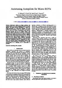
Figure 1.1: This graph shows that while the growth in transistors (and thus Moore’s Law [36]) continues unabated, clock speed and power stabilized in 2004. This is the same time that multicore chips first started appearing. This data was collected by Herb Sutter, Kunle Olukotun, Christopher Batten, Krste Asanovi´c, and Katherine Yelick. utilize much simpler, lower-frequency cores to attain large power and performance benefits. Thus, we need to start designing codes now that can handle increasing amounts of parallelism [44].
1.2
Performance Portability Challenges
Unfortunately, merely writing explicitly parallel code is not enough. We will see in Chapters 7 and 8 that na¨ıvely threaded programs, even for very simple kernels, fail to effectively utilize a multicore machine’s resources. This can be largely attributed to the complexity of current hardware and software and the inability of general purpose compilers to handle that complexity. These compilers have two major limitations that cause codes to underperform. First, in order to hasten compilation time, they almost always rely on heuristics, not experiments, to determine the optimal values of needed parameters. We will see in Section 3.1 that today’s multicore platforms are
3 sufficiently diverse and complex that heuristics no longer suffice. Second, software is often written with complex data and control structures so that these compilers also fail to infer the legal domain-specific transformations that are needed to produce the largest performance gains. However, this is to be expected, given some of the challenging algorithmic and data structure changes that may be required. One solution to this problem is to hand-tune the relevant computational kernel for a given platform; this would allow the programmer to specify the domain-specific transformations that the compiler alone was unable to exploit. While this may work in the short term, as soon as the tuned code needs to be ported, possibly to a different architecture with more cores, it will likely need to be retuned. In Sections 7.5 and 8.4, we show that that the best code and runtime parameters for one multicore machine often do not correspond to good performance on other machines. In fact, a stencil code tuned for one platform, if ported to another platform without further tuning, may achieve less than half of the new platform’s best performance. This assumes that there is enough parallelism in the code to keep all of the new platform’s threads busy and load balanced. If this is not true, then the performance drops even further.
1.3
Auto-tuning
A better solution is to automatically tune, or auto-tune, the relevant kernel. This does require a significant one-time cost to the programmer, but once the auto-tuner is constructed, it shifts the burden of tuning from the programmer to the machine. As a result, it is highly portable. Moreover, it increases programmer productivity when the one-time cost to build the auto-tuner can be amortized by running across several different machines. There are other advantages to auto-tuning. Auto-tuners can be designed to handle any core count, thereby making them scalable. This will be a valuable asset in the manycore era. Furthermore, auto-tuners can also be constructed for maximizing metrics other than performance (e.g. power efficiency), thus also making them flexible. Due to all of these reasons, auto-tuning has already had several previous success stories, including: FFTW [20], SPIRAL [41], OSKI [54], and ATLAS [55].
4
1.4
Thesis Contributions
In this thesis, we construct auto-tuners for codes that perform relatively simple, but common, nearest-neighbor, or stencil, computations. The following are our primary contributions. • We have identified a set of new and known optimizations specifically for stencil codes, including: core blocking, thread blocking, register blocking, NUMAaware data allocation, array padding, software prefetching, cache bypass, SIMDization, and common subexpression elimination. Collectively, they are designed to optimize the data allocation, memory bandwidth, and computational rate of stencil codes. • Based on these optimizations, we have developed three stencil auto-tuners that can achieve substantially better performance than na¨ıvely threaded stencil code across a wide variety of cache-based multicore machines. After full tuning, we realized speedups of 1.9×–5.4× over the performance of a na¨ıvely threaded code for the 3D 7-point stencil, between 1.8×–3.8× for the 3D 27-point stencil, and between 1.3×–2.5× for the 3D Helmholtz kernel with a 2 GB fixed memory footprint. • We have developed an “Optimized Stream” benchmark that uses many of the same optimizations as in the stencil auto-tuners to achieve the best possible streaming memory bandwidth from a given machine. It is able to achieve bandwidths between 0.3%–13% higher than those attained from the untuned “Stream” benchmark [35]. The Optimized Stream benchmark is also one piece of the Roofline model [58], and thus allows us to place a performance “roofline” on bandwidth-bound kernels. • We have analyzed the performance of our auto-tuner against the bandwidth and computational limits of each machine. For the 7-point stencil, we are able to achieve between 74%–95% of the attainable bandwidth for the memory-bound machines, as well as 100% of the in-cache performance for the compute-bound IBM Blue Gene/P. For the 27-point stencil, we realized between 85%–100%
5 of the in-cache performance for the compute-bound architectures, 89% of the attainable bandwidth for the bandwidth-bound Intel Clovertown, and 65% of both attainable bandwidth and computation on the AMD Barcelona. Finally, for a single iteration of the Helmholtz kernel, we performed at between 89%– 100% of the peak attainable bandwidth. Therefore, in almost all cases, we are able to effectively exploit either the bandwidth or computational resources of the machine. • In Chapter 9, we no longer tuned a single large problem. Instead, we autotuned many small subproblems that mimicked the behavior of the Adaptive Mesh Refinement (AMR) code that this kernel was ported from. In order to tune these multiple subproblems well, we introduced the adjustable threads per subproblem parameter. Fewer threads per subproblem corresponded to coarsegrained parallelism, while more threads per subproblem meant fine-grained parallelism. We discovered that utilizing fewer threads per problem usually performed best, but also introduced load balancing issues. If future manycore architectures do not provide better support for fine-grained parallelism, load balancing will be an even larger issue than it is today.
1.5
Thesis Outline
The following is an outline of the thesis: Chapter 2 gives an overall description of stencils, along with examples from some of the many applications from which they arise. Stencils are also described as a very specific, but efficient, form of sparse matrix-vector multiply. Chapter 3 goes into depth about each of the cache-based multicore machines that were employed in this study. We also discuss some of the experimental details that are used in the later chapters, including the choice of compilers, the manner in which threads are assigned to cores, and how timing data is collected. Chapter 4 introduces the stencil-specific optimizations that were used in this study. These optimizations are grouped into four rough categories: problem decomposition, data allocation, bandwidth optimizations, and in-core optimizations.
6 Chapter 5 subsequently explains how these optimizations were combined into a stencil auto-tuner, including details about code generation and parameter space searching. Chapter 6 details how the Roofline model [58] provides performance bounds for stencil codes. The Roofline model is a general model that incorporates both bandwidth and computation limits into its performance predictions. Chapters 7, 8, and 9 then discuss the tuning and resulting performance of the 7point stencil, 27-point stencil, and the Helmholtz kernel, respectively. Together, these three stencils are representative of many real-world stencil codes. By understanding how we were able to achieve good performance for these stencils, similar techniques can be applied to many more stencil codes. Chapters 10 discusses related and future work, and we conclude in chapter 11.
7
Chapter 2 Stencil Description 2.1
What are stencils?
Partial differential equation (PDE) solvers are employed by a large fraction of scientific applications in such diverse areas as diffusion, electromagnetics, and fluid dynamics. These applications are often implemented using iterative finite-difference techniques that sweep over a spatial grid, performing nearest neighbor computations called stencils. In a stencil operation, each point in a regular grid is updated with weighted contributions from a subset of its neighbors in both time and space– thereby representing the coefficients of the PDE for that data element. These coefficients may be the same at every grid point (a constant coefficient stencil) or not (a variable coefficient stencil). Stencil operations are often used to build solvers that range from simple Jacobi iterations to complex multigrid [6] and adaptive mesh refinement (AMR) methods [3]. Stencil calculations perform sweeps through data structures that are typically much larger than the capacity of the available data caches. In addition, the amount of data reuse is limited to the number of points in the stencil, which is typically small. The upshot is many (but not all) of that these computations achieve a low fraction of theoretical peak performance, since data from main memory cannot be transferred fast enough to avoid stalling the computational units on modern microprocessors. Reorganizing these stencil calculations to take full advantage of memory hierarchies has been the subject of much investigation over the years. These have principally
8
(a) 1D 5-Point Stencil
(b) 2D 5-Point Stencil
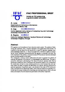
Figure 2.1: A visualization of two lower dimensional stencils. In (a), we show a onedimensional five-point stencil, where the center point is both being read and written. In (b), we show a two-dimensional five-point stencil, where again the center point is read and written. focused on tiling optimizations [43, 42, 32] that attempt to exploit locality by performing operations on cache-sized blocks of data before moving on to the next block. However, a study of stencil optimization [27] on (single-core) cache-based platforms found that these tiling optimizations were primarily effective when the problem size exceeded the on-chip cache’s ability to exploit temporal recurrences. We will show shortly that for lower dimensional stencils, modern microprocessors have caches large enough to exploit these temporal recurrences. For stencils with dimensionality higher than two, however, tiling optimizations are still effective and needed.
2.1.1
Stencil Dimensionality
1D and 2D Stencils In Figure 2.1, we show two examples of simple lower dimensional stencils. While lower dimensional stencils are fairly common, they are likely to be less amenable to tuning as well as heavily bandwidth-bound. First, we know from previous work [28] that the lower the stencil dimensionality, the less likely it is to be affected by capacity cache misses [24]. This is because the required working set size is smaller. If we examine Figure 2.2(a), we see the conventional memory layout for a 2D 5-point stencil like the one in Figure 2.1(b). If N X is the unit-stride grid dimension of the 2D grid, then for the 5-point stencil, the first and last stencil points are separated by (2 × N X) doubles in the read array. When streaming through memory, by the time the last stencil point is read in, all the pre-
9 working set size NX
read_array[]
write_array[] (a) Memory layout for the 2D 5-point stencil working set size NX
NX*NY
read_array[]
write_array[] (b) Memory layout for the 3D 7-point stencil
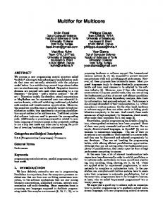
Figure 2.2: A visualization of the memory layout for two stencils of different dimensionality. In (a), we see that the first and last stencil points of the 2D 5-point stencil are separated by (2 × N X) doubles, where N X is the unit-stride dimension of the 2D grid. In (b), the distance between the first and last stencil points for the 3D 7-point stencil is much larger– specifically, (2 × N X × N Y ) doubles, where N X and N Y are the contiguous and middle dimensions of the 3D grid, respectively. vious stencil points will still be in cache since the working set is miniscule compared to the last-level cache of current multicore processors. To make this concrete, the working set when performing a 2D five-point stencil on a 2562 grid is about 4 KB. In comparison, the last-level caches of the machines in this thesis range from 2–8 MB. By avoiding capacity misses, 2D stencils will not benefit from cache tiling optimizations like core blocking, which we will introduce in Section 4.1.1. In this respect, 2D stencil codes have less headroom for performance improvement than codes that do incur capacity misses. Second, the number of flops performed per point also usually decreases with lower stencil dimensionality. This is simply because there are fewer dimensions in which stencil points can occur. However, regardless of dimensionality, the memory traffic for each grid point remains constant. Therefore, for the same number of grid points, there are fewer flops performed for lower dimensional stencils. Consequently, these stencils are more susceptible to bandwidth limitations. While the performance of lower dimensional stencil codes can be improved through
10
+Z
weight point by α
+Z
weight point by β +Y
weight point by γ
+Y +X (unit stride)
(a) The 7-point stencil shown as three adjacent planes.
+X
weight point by δ
(unit stride)
(b) The 27-point stencil shown as three adjacent planes.
Figure 2.3: A visual representation of the 3D 7-point and 27-point stencils, both of which are shown as three adjacent planes. These stencils are applied to each point of a 3D grid (not shown), where the result of each stencil calculation is written to the red center point. Note: the color of each stencil point represents the weighting factor applied to that point. tuning, they are heavily bandwidth-bound and typically do not benefit from cache tiling. As a result, the achievable speedup is fairly constrained compared to 3D stencils. In this thesis, we do not tune 1D and 2D stencils. 3D Stencils The focus of this thesis is on 3D stencils, two of which are shown in Figure 2.3. The 7-point stencil, shown in Figure 2.3(a), weights the center point by some constant α and the sum of its six neighbors (two in each dimension) by a second constant β. Na¨ıvely, a 7-point stencil sweep can expressed as a triply nested ijk loop over the following computation: Bi,j,k = αAi,j,k + β(Ai−1,j,k + Ai,j−1,k + Ai,j,k−1 + Ai+1,j,k + Ai,j+1,k + Ai,j,k+1 ) (2.1) where each subscript represents the 3D index into array A or B. The 27-point 3D stencil, as shown in Figure 2.3(b), is similar to the 7-point stencil, but with additional points to include the edge and corner points of a 3×3×3 cube surrounding the center grid point. It also introduces two additional constants– γ, to weight the sum of the edge points, and δ, to weight the sum of the corner points.
11 These two stencils are the focus of our tuning in Chapters 7 and 8, and they will also be discussed in further detail later in this chapter. Unlike the lower dimensional stencils that were just discussed, the required working set size for 3D stencils is much greater than 1D or 2D stencils. We see in Figure 2.2(b) that if N X and N Y are the contiguous and middle dimensions of our 3D grid, respectively, then for the 3D 7-point stencil, the first and last points will be separated by (2 × N X × N Y ) doubles in the read array. This is significantly larger than the (2 × N X) separation for the 2D 5-point stencil, since the distance is now in terms of planes, not pencils. For example, if we performed a sweep of the 3D 7-point stencil over a 2563 grid, the working set is about 1 MB, which is approximately 250× the working set size for the 2D analog problem. Consequently, cache capacity misses are far more likely, but optimizations like core blocking should now be effective. Furthermore, the number of flops per grid point will be higher in 3D codes as well. As we will discuss later, the 3D 7-point stencil in Figure 2.3(a) performs eight flops per point, since the center point is weighted by α and each of the six nearest neighbors is weighted by β. More generally, this stencil gives one weight (α) to the center point, and a separate weight (β) to each of the two neighboring stencil points in each dimension. Thus, the d-dimensional analog of this stencil will perform (2d+2) flops per point, which increases linearly with dimensionality. The increase in flop count is even more dramatic when we alter the dimensionality of the 3D 27-point stencil, displayed in Figure 2.3(b). This stencil has four weights associated with it– one each for the one center point (α), six face points (β), twelve edge points (γ), and eight corner points (δ). The full computation requires 30 flops per grid point. More generally, the d-dimensional analog of this stencil utilizes (d+1) weights and performs (3d + d) flops per point. In this case, the flops per point rise exponentially with dimensionality. Due to the occurrence of capacity misses and the greater number of flops per point, we anticipate that a larger number of transformations (including cache blocking and computational optimizations) will be effective for 3D stencils than for lower dimensional stencils. We also expect that the resulting speedups will be larger as well.
12 Higher-Dimensional Stencils For higher dimensional stencils, the points that were made for three-dimensional stencils are further amplified. If we continue storing the structured grid data in the usual manner (shown in Figure 2.2), then the distance in memory between the first and last point will again be multiplied by the size of another dimension. If we na¨ıvely stream through memory without any tiling optimizations, the required working set will almost definitely be larger than the available last-level cache. We should also expect more flops per point, given that there are more dimensions present. Lattice Methods Lattice methods are still structured grid codes, but instead of a single unknown per point, many can be present. Whether lattice methods should be considered very high dimensional stencils or a separate category unto themselves is debatable. However, we would be remiss if they were not mentioned. One example of a lattice method is a plasma turbulence simulation that was tuned by Williams et al [56]. This lattice Boltzmann application coupled computational fluid dynamics (CFD) with Maxwell’s equations, resulting in a momentum distribution, a magnetic distribution, and three macroscopic quantities being stored per point. In total, each point required reading 73 doubles and updating 79 doubles, while performing approximately 1300 flops. This resulted in complex data structures and memory access patterns, as well as significant memory capacity requirements, so proper tuning (especially at the data structure level) was critical.
2.1.2
Common Stencil Iteration Types
This subsection goes into depth about three common stencil iteration types: Jacobi, Gauss-Seidel, and Gauss-Seidel Red-Black iterations. Jacobi As shown in Figure 2.4(a), Jacobi iterations are essentially out-of-place sweeps. In order to perform Jacobi iterations, there is at least one read grid and one write
13
Read Grid
Write Grid
(a) Jacobi Iteration
Read and Write Grid (b) Gauss-Seidel Iteration
Read and Write Grid (c) Gauss-Seidel Red-Black Iteration
Figure 2.4: A visual representation of the some of the common iteration types that occur with stencil codes. In a Jacobi iteration, a stencil is applied to each point in the read grid, and the result is written to the corresponding point in the write grid. The Gauss-Seidel iteration is similar, except that there is only a single grid, and therefore the iteration is in-place. The Gauss-Seidel Red-Black iteration is also in-place, but all the points of one color are updated before the points of the other color are updated. grid, but no grids are both read and written. We sweep through these grids by first incrementing the unit-stride index, then incrementing the middle index, and finally incrementing the least-contiguous index. Essentially, we stream consecutively through memory. The power of Jacobi sweeps lies in the fact that it is easily parallelizable; any point in the write grid(s) can be computed independently of any other point, so they can be updated in an embarrassingly parallel fashion. Thus, since all partitioning schemes produce the same correct result, we are free to choose the one that performs best. Another benefit of the Jacobi iteration is that on x86 architectures, we can use the cache bypass optimization (discussed in Section 4.3.2) to reduce the memory traffic on a write miss by half by eliminating the cache line read. Most stencil codes are bandwidth-bound, so this has the potential to generate large performance speedups. The major drawback to the Jacobi iteration is that it requires that we store distinct read and write arrays, which increases both storage and bandwidth requirements. When we perform 7-point stencil and 27-point stencil updates in Chapters 7 and 8, respectively, we will be performing a single Jacobi sweep. This allows us great flexibility in how we parallelize the problems.
14 Gauss-Seidel Gauss-Seidel iterations, shown in Figure 2.4(b), are in-place sweeps. Zero or more read-only grids may be present, but the write grid must also be read from first. One consequence of this fact is that almost all the computed stencils will include some points that were already updated during the current sweep and others that were not. This means that there is an inherent dependency chain that needs to be respected if we wish to replicate the same final answer. Unfortunately, this significantly limits the amount of available parallelism in the sweep. It also causes different traversals through the grid to generate different (but valid) results. The major benefit to GaussSeidel sweeps is that the write grid is also read from, thereby reducing the need for additional arrays and the memory traffic associated with them. Gauss-Seidel Red-Black Gauss-Seidel Red-Black (GSRB) iterations are similar to Gauss-Seidel sweeps in that while read-only grids may be present, the write grid must be read from first. In order to deal with the limited parallelism that is exposed when consecutively updating each point (like in Gauss-Seidel sweeps), GSRB updates only every other point. For instance, in Figure 2.4(c), a black grid point will only be updated when the red points that it depends on have all been updated. Once the needed black points are ready, we can again start updating the red points, and so on. This type of sweep has similar parallelism characteristics to Jacobi, since any of the points of a single color can be updated independently of any other. Thus, the partitioning of this sweep among threads can be arbitrary. If we define a GSRB sweep as performing a single update for both the red and black grid points, then a na¨ıve GSRB implementation will sweep over the grid twice, likely requiring twice the memory traffic of a Jacobi or Gauss-Seidel sweep. However, we can minimize the required memory traffic by having a leading “wavefront” for the red points and a trailing wavefront for the black points. Assuming the last-level cache is sufficiently large, this would update both sets of points while only reading them from memory once. The Helmholtz kernel, discussed in Chapter 9, will perform GSRB sweeps over
15 each subproblem. Numerical Convergence Properties While the numerical convergence properties of these iterative methods are generally out of the scope of this thesis, they are a major concern for tuning real-world stencil codes, and thus we touch upon them here. Out of the three iteration types just discussed, the Jacobi iteration is typically the slowest to converge. A superficial explanation for this is because every point is updated with old (i.e. not updated during the current iteration) grid point values. This is rectified by performing GaussSeidel sweeps, since most points are calculated from some old and some new values. Indeed, in most cases, Gauss-Seidel shows better convergence than Jacobi. However, the best convergence usually comes from GSRB; one GSRB step can decrease the error as much as two Jacobi steps. This is a general phenomenon for matrices arising from approximating differential equations with finite difference approximations [14]. It is important to note that when solving a linear system, it is possible that one step of Jacobi could reduce the error more than one step of GSRB. This is because the amount of convergence depends both on the problem and the iterative method. In most cases, though, GSRB will converge fastest and Jacobi slowest. Ultimately, many iterative solvers attempt to reduce the problem error (or residual) below a certain threshold. In order to decide how to minimize the time needed to reach this level of convergence, we need to understand how many iterations a given solver will require (based on its numerical properties), as well as how long each iteration will take (based on numerical, hardware and software properties).
2.1.3
Common Grid Boundary Conditions
Another concern with structured grid codes is how to deal with boundary conditions. Here we discuss two common boundary conditions and how to deal with them.
16
G G G G G G G G G G G G G G G G (a) A 2D grid with ghost cells for storing boundary conditions.
(b) A 2D grid with periodic boundary conditions and no extra cells.
Figure 2.5: In (a), we show a 3×3 grid with surrounding ghost cells (marked with a “G”) that are used to store boundary conditions. In (b), we show a 3×3 grid which does not require ghost cells because it has periodic boundary conditions. Constant Boundaries There are two main types of constant boundary conditions. In the first case, the points along the boundary do not change with time, but do change depending on position. In this case, we can use ghost cells (like in Figure 2.5(a)) to store these values before any stencil computations begin. Once the ghost cells are initialized, they do not need to be altered for the rest of the problem. In this thesis, all three 3D stencil kernels have this type of boundary condition. However, the ghost cells consume a non-trivial amount of memory for 3D grids. Suppose that we have an N 3 grid that is surrounded by ghost cells. Then, the resulting grid has (N + 2)3 cells. If N = 16, then ghost cells represent an astounding 30% of all grid cells. However, if N = 32, then the percentage drops to 17%. The second case is if the boundary value does not change with time or position. In this case, the entire boundary can be represented by a single constant scalar throughout the course of the problem. Consequently, we no longer need to have individual ghost cells like the previous case. Periodic Boundaries Another common boundary condition is to have periodic boundaries, as shown in Figure 2.5(b). For points along the boundary, this means that they have additional neighbors that wrap around the grid. For example, the left neighbor of the upper left
17 point is the upper right point, while the upper neighbor is the lower left point. While periodic boundaries can be represented using ghost cells that are updated after each iteration, in many cases no ghost cells are used at all. Instead, the required values are merely read from the side of the grid. This helps lower the memory footprint of the grid as well as bandwidth requirements.
2.1.4
Stencil Coefficient Types
Constant Coefficients In the stencils we have thus far discussed, we have usually assumed that the stencil coefficients are constant. For instance, in Figure 2.3, the color of each stencil point represents whether that point is weighted by the constant coefficient α, β, γ, or δ. Many finite difference calculations employ constant coefficient stencils like these. When the coefficient values are constant scalars, they do not need to be continually read from memory for every new stencil. Instead, they can be hard-coded into the inner loop of the stencil code, and then kept in registers during the actual computation. This results in a large reduction in potential storage requirements and memory traffic. Furthermore, if these coefficients are simple integer values, the compiler may even be able to further optimize parts of the computation. In many ways, the constant coefficient stencil is an ideal scenario. Consequently, if we can expose the appropriate properties in an iterative solver’s underlying matrix so as to generate a constant coefficient stencil, we will always do so. In Section 2.2, we will specify these properties. The 7-point and 27-point stencils that we tune in Chapters 7 and 8, respectively, both have constant coefficients. Variable Coefficients However, the stencil coefficients need not be constant. As we will examine in Section 2.2, the iterative solver’s underlying matrix may not have the appropriate properties for it. In such a case, we may still be able to utilize a variable coefficient stencil, where the stencil weights change from one grid point to another. Unlike constant coefficient stencils, we now need to store these weights in separate grids.
18 When performing our calculations, we will stream through these grids along with our original grid of unknowns. This will create extra DRAM traffic, but we will show in Section 2.2.3 that this is still preferable to performing a sparse matrix-vector multiply. The Helmholtz kernel that we will tune in Chapter 9 employs a variable coefficient stencil.
2.2
Exploiting the Matrix Properties of Iterative Solvers
Thus far, we have discussed various stencil characteristics, but we have not mentioned the origins of stencils in any detail. This section explains how both variable and constant coefficient stencils can arise from iterative solvers. Imagine that we have a structured grid like the one shown in Figure 2.6. This grid is a simple two-dimensional grid with periodic boundary conditions in both dimensions. Now, let us suppose that we would like to apply an iterative solver to this grid. In most cases, this solver will require that every point in the structured grid be updated with some linear combination of other grid points. In order to generally represent this linear transformation, we can create a matrix that stores the weights that each point contributes to every point in the grid. In order to create this matrix, we first need to select an ordering of the grid points. In our case, the simplest way to proceed is to choose a natural row-wise ordering, where we first order the top row from left to right, then the second row in a similar manner, and so on. The numbers inside each grid point of Figure 2.6 show such an ordering [30]. We can now create a matrix A that represents the linear transformation performed by the iterative solver. The amount that point j will be weighted by when calculating the new value of point i is given by matrix element Aij .
2.2.1
Dense Matrix
At this juncture, a critical question is how best to store this matrix. At the most general level, we can store A as a dense matrix. However, for a n × n square grid
19
1 2 3 4 5 6 7 8 9
Figure 2.6: A 3×3 numbered grid with periodic boundary conditions in both the horizontal and vertical directions. The grid points are numbered in a natural rowwise ordering. with no extra ghost cells, the resulting matrix A will have dimensions of n2 × n2 . Thus, the 3 × 3 grid from Figure 2.6 would be stored as a 9 × 9 matrix. Despite the large size of A in a dense matrix format, most iterative solvers only reference a few grid points in updating each point, so we expect A to be sparse (i.e. most of the elements are zero). Therefore, storing A in a dense matrix would be inefficient in terms of both storage and flops.
2.2.2
Sparse Matrix
A better choice would be some sort of sparse matrix format. Let us assume that there are nnz non-zeros in the A matrix, each of which will be stored as an 8 Byte double-precision number. In addition, the matrix indices will be stored as 4 Byte integers. Given this, if we choose the commonly-used Compressed Sparse Row (CSR) format [53] to store A, we will require about 12nnz+4n2 Bytes of storage and perform approximately 2nnz flops. This is much better than the 8n4 Bytes of storage and 2n4 flops required by the dense format. While the CSR format does perform indirect accesses into the matrix, it should still be orders of magnitude faster than the dense format for sufficiently large and sparse matrices.
2.2.3
Variable Coefficient Stencil
Sparse matrices are a general way to represent the linear transformation performed by an iterative solver. However, in many cases, these iterative solvers perform nearest neighbor operations on the structured grid. For instance, imagine that for every point grid in Figure 2.6, we only require the values of the points immediately
20
2
9 −7 −12 −3
7
−13
101
20
14
5.3
13 −67
8 −31
−2 5
−15
23
17
1.3
7
−9
5
0.4
3
1 42
0.1 81
4.2
8
87 8 14 51 9
17
10
−41
2
−1
32
91
71
Table 2.1: This sparse matrix has a very regular structure, but the non-zero values are unpredictable. For readability, the matrix is divided into 3×3 submatrices and only the non-zeros are shown.
above, below, to the left, and to the right of that point, as well as the value of the point itself. Thus, every point will be updated with the values from five grid points, but the weights associated with these grid points are not predictable. The 9 × 9 matrix in Table 2.1 represents such a situation for the case of periodic boundary conditions. Due to its regular structure, we no longer explicitly need to store the matrix indices. Instead of storing this n2 × n2 matrix in a sparse format, we can store it as five n × n grids. For a given point (i, j) from the grid in Figure 2.6, the corresponding (i, j) point in each of these grids represents the weight associated with point (i, j) or any of its four neighbors. More information about these variable coefficient stencils can be found in Section 2.1.4. Thus, we now require 40n2 Bytes of storage and perform 9n2 flops. In a sparse matrix format, we would need 64n2 Bytes of storage, where the extra 24n2 Bytes is attributed to the unneeded indices of the CSR format. However, we have not altered the flop count by changing the data structure from a sparse matrix to a variable coefficient stencil.
2.2.4
Constant Coefficient Stencil
Finally, if we have a matrix with the same structure as Table 2.1, but also with predictable non-zeros, we no longer need to explicitly store the non-zeros either.
21
−4
1
1
1
−4
1
1
1
−4
1 1 1 1
1 1
1 1
−4
1
1
1
−4
1
1
1
−4
1 1
1 1
1
1
1 1 1 1 −4
1
1
1
−4
1
1
1
−4
Table 2.2: This is the matrix associated with the 2D Laplacian operator with periodic boundary conditions. It has a very regular structure and the non-zero values are predictable.
Instead of storing five separate arrays, we only need to store five separate scalar constants! Moreover, if we wish to apply an operator like the 2D Laplacian, we only need to store two constants. This is because the center point will always be weighted by -4, while all of four of its neighbors will be weighted by 1. The matrix associated with the 2D Laplacian operator with periodic boundary conditions is shown in Table 2.2. Now, we only need to store 16 Bytes worth of data– the weight of the stencil’s center point and the weight of its four neighbors. Moreover, this reduces our flop count from 9n2 down to 6n2 . We have finally succeeded in reducing the dense matrix representing our iterative solver down to a simple constant coefficient stencil.
2.2.5
Summary
The above arguments for reducing storage, bandwidth, and computation requirements were made for two-dimensional structured grids, and are summarized in Table 2.3. However, the corresponding savings are even more stark for three-dimensional stencils, which are the focal point of this thesis.
22 Explicit Indices Implicit Indices Usual Sparse Variable Explicit Non-zeros Matrix-Vector Coefficient Multiply Stencil Example: Constant Implicit Non-zeros Laplacian of a Coefficient General Graph Stencil Table 2.3: This table displays the continuum from sparse matrix-vector multiply to variable-coefficient stencils and finally constant-coefficient stencils.
2.3
Tuned Stencils in this Thesis
This thesis focuses on two second-order finite difference operators as well as a finite volume operator. The finite difference operators are constant coefficient stencils, while the finite volume operator is a variable coefficient stencil. In this section, we describe each in more detail, including some information on where the stencils originate from.
2.3.1
3D 7-Point and 27-Point Stencils
The 3D 7-point and 27-point stencils, visualized in Figure 2.3, commonly arise from the finite difference method for solving PDEs [30]. The 7-point stencil performs eight flops per grid point, while the 27-point stencil performs 30 flops per point (without any type of common subexpression elimination). Thus, the arithmetic intensity, the ratio of flops performed for each Byte of memory traffic, is about 3.8× higher for the 27-point stencil than the 7-point stencil. We will see in Chapter 8 that the compute-intensive 27-point stencil will actually be limited by computation on some multicore platforms. The 7-point 3D stencil is fairly common, but there are many instances where larger stencils with more neighboring points are required. One such stencil arises from T. Kim’s work in optimizing a fluid simulation code [29]. By using a Mehrstellen scheme [10] to generate a 3D 19-point stencil (where δ equals zero in Figure 2.3) instead of the usual 7-point stencil, he was able to reach the desired error reduction in 34% fewer stencil iterations. Thus, larger stencils can reduce the number of iterations
23 needed to reach a desired threshold of convergence. In this thesis, we chose to examine the performance of the 27-point 3D stencil because it serves as a good proxy for many of these compute-intensive stencil kernels. In general, though, the numerical properties of the 7-point and 27-point stencils are outside the scope of this work; we merely study and optimize their performance across different multicore architectures. Our results will hopefully allow the reader to judge as to whether these numeric/performance tradeoffs are worthwhile. As an added benefit, this analysis also helps to expose many interesting features of current multicore architectures.
2.3.2
Helmholtz Kernel
The final stencil that we tune is the Helmholtz kernel. This kernel is ported from Chombo [9], a software framework for performing Adaptive Mesh Refinement (AMR) [3]. The Helmholtz kernel that we tune in Chapter 9 attempts to solve for φ in the equation: L(φ) = rhs
(2.2)
where rhs is a given right-hand side and L is the linear Helmholtz operator: ~ I~ − β ∇ ~ ·B ~∇ ~ L = αA
(2.3)
We can solve Equation 2.2 iteratively by calculating the residual, multiplying it by λ, and subtracting this quantity from our original φ (called φ∗ below): φnew = φ∗ − λ(L(φ∗ ) − rhs)
(2.4)
If we perform enough iterations of Equation 2.4, we should converge (albeit slowly) to a φ whose residual is below a given threshold. However, to hasten this process, we can use solvers like multigrid [6, 52], where these iterations can be used to relax each multigrid level. In the case of AMR, where many small grids are present, multigrid is applied to the entire collection of subproblems [33], while a relaxation operator (like GSRB) is applied to each of the individual subproblems. The power of the Helmholtz equation comes from its ability to solve time-dependent problems implicitly within a multigrid solver. Explicit time discretization schemes
24 Single Helmholtz Subproblem Subgrid Read/Write Dimensions phi Read and Write (N X + 2) × (N Y + 2) × (N Z + 2) aCoef0 Read Only NX × NY × NZ bCoef0 Read Only (N X + 1) × N Y × N Z bCoef1 Read Only N X × (N Y + 1) × N Z bCoef2 Read Only N X × N Y × (N Z + 1) lambda Read Only NX × NY × NZ rhs Read Only NX × NY × NZ Table 2.4: A description of the seven grids involved in a single variable-coefficient Helmholtz subproblem. The N X, N Y , and N Z grid parameters are visually displayed in Figure 4.1.
place bounds on the size of the time step due to the Courant-Friedrichs-Lewy (CFL) stability condition. Implicit time discretization schemes, however, have no time step restriction, and are unconditionally stable if arranged properly. One example of this is the parabolic heat equation. While this equation can be solved using an explicit forward Euler scheme, the CFL condition will keep our time steps short. The discrete Helmholtz equation, on the other hand, can apply several different implicit schemes merely by varying α and β in Equation 2.3. In particular, we can apply a backward Euler, Crank-Nicholson, or backward difference formula through the Helmholtz equation, all of which allow for much larger time steps than forward Euler. A second example is the hyperbolic wave equation. Again, the CFL condition only limits the time steps of explicit methods. For most common implicit discretizations, each time step can again be solved implicitly using the discrete Helmholtz equation with an appropriately tuned α and β. These examples apply to more general timedependent parabolic and hyperbolic PDEs as well. The beauty of this approach is that the larger the time steps, the more will be gained through an appropriate multigrid treatment [52]. Now, if we actually discretize the Helmholtz equation (Equation 2.4), the result is a variable coefficient stencil consisting of seven grids. Six of these grids are read only, while the phi grid is both read and written; the dimensions of each of these grids
25
(a) Cell-centered grid
(b) Face-centered grid
Figure 2.7: This diagram shows that the cell-centered grid in (a) requires far fewer grid points than the face-centered grid in (b). The grid points in (b) are color-coded, where the points along a cell’s horizontal edges are green and the points along the vertical edges are in blue. are given in Table 2.4. As this is a variable coefficient stencil, we note that the phi array cannot be merely updated with scalar weights; there are five grids (other than phi or rhs) that need to be referenced in order to perform this stencil calculation. ~ is Some of the arrays in Table 2.4 require further explanation. For instance, B represented as three separate arrays– bCoef0, bCoef1, and bCoef2. This is because the stencil originates from a finite volume, not finite difference, calculation. So as to abide by certain conservation laws, B employs a face-centered, not cell-centered, discretization. As we can see in Figure 2.7, the face-centered grid in (b) requires many more grid points than cell-centered grid in (a). The primary reason for this is that the face-centered discretization requires that there be a grid point along each edge of a given cell. For instance, Figure 2.7(b) shows the points along each cell’s horizontal edges in green and the points along the vertical edges in blue. For this calculation, the face-centered grid points along each dimension are stored separately. ~ is thus stored as three separate arrays As this is a three-dimensional problem, B (bCoef0, bCoef1, and bCoef2). In addition, each of these arrays needs a single extra grid point in one dimension in a similar fashion to how there are four columns, but five rows, of green points in Figure 2.7(b). The phi array deserves some explanation as well, since it has two extra cells in each dimension. The extra cells in this case are simply ghost cells that store boundary values. To be mathematically correct, these ghost cells should be updated after each iteration. In some cases, however, it is possible to perform multiple iterations without a ghost cell update while still preserving stability and accuracy. This is an area of
26 current research [31]. When executing a sweep of this variable coefficient stencil, we can choose any of the iteration types displayed in Figure 2.4, but GSRB was chosen for its convergence and parallelization properties. However, due to the number of arrays present and the fact that we are employing a GSRB stencil, the arithmetic intensity of this kernel is fairly low, despite performing 25 flops per point.
2.4
Other Stencil Applications
Thus far, we have discussed a few areas where stencils originate. The following section introduces other uses of stencils, but this is far from an exhaustive list.
2.4.1
Simulation of Physical Phenomena
Stencils are often found when modeling physical phenomena. For instance, Nakano et al used stencils as part of a molecular dynamics algorithm for realistic modeling of nanophase materials [38]. Specifically, in order to compute the Coulomb potential, which is very expensive due to its all to all nature, the authors decided to use the fast multipole method (FMM). In the FMM, the Coulomb potential is computed using a recursive hierarchy of cells. At each level of this hierarchy, the near-field contribution to the potential energy is calculated through nearest neighbor stencil calculations. The FMM algorithm is able to reduce this O(N 2 ) all-to-all calculation down to a complexity of O(N ). Stencils are also used in quantum mechanics simulations. Shimono et al [45] developed a hierarchical method that decomposed the spatial grid based on higher-order finite differences and multigrid acceleration [6]. This method also refines adaptively near each atom to accurately operate the ionic pseudopotentials on the electronic wave functions. This divide-and-conquer scheme is used to iteratively and quickly solve for the potential throughout the grid. As an added benefit, this approach provides simple and efficient parallelization of the problem due to the short-ranged operations involved. A final simulation example comes from the area of earthquake modeling. Specifi-
27 cally, Dursun et al have tuned a seismic wave propagation code for x86 clusters [15]. The code employs a higher-order 3D 37-point stencil based off of the finite difference method. Such a stencil not only involves heavy computation but also large memory requirements (since the points are not clustered around the center point). The authors used spatial decomposition, multithreading, and SIMD (explained in Section 4.4.2) to achieve speedups of up to 7.9×. These optimizations are a subset of the ones we employ in this thesis, described in Chapter 4.
2.4.2
Image Smoothing
We now take a step away from simulations and instead focus on image smoothing, a fundamental operation in computer vision and image processing. This smoothing is often done through a bilateral filter, which tries to remove noise while not smoothing away edge features. Consequently, a bilateral filter uses a variable coefficient stencil, where the weights are computed as the product of a geometric spatial component and signal difference. Kamil et al tuned this stencil kernel [26] using many of the same techniques that we employed in this thesis.
2.5
Summary
This chapter has introduced stencils, as well as some of the issues that occur when confronting variations in dimensionality, iteration type, boundary condition, or coefficient type. Many of these issues will play out as we tune the three stencils in Chapters 7, 8, and 9. Part of this chapter was also dedicated to explaining the origins of stencils that are used as iterative solvers. As we saw, we need to exploit the underlying matrix structure to generate variable coefficient stencils, but we also need to take advantage of predictable non-zeros if we wish to use constant coefficient stencils. Fortunately, this happens fairly often, as we discovered stencils being utilized as iterative solvers in material modeling, quantum mechanics, and seismic wave modeling codes. We also observed a non-simulation use of stencils– performing image smoothing using a bilateral filter. Thus, stencils are found in many scientific disciplines, and some
28 non-science ones as well. This ubiquity emphasizes the importance of achieving good stencil code performance on multicore platforms.
29
Chapter 3 Experimental Setup This chapter details our experimental methodology at almost every level of the system stack. At the hardware level, we discuss specifics about the multicore platforms used in our evaluations and the thread mapping policy we implemented. At the software level, we justify our choice of parallel programming model, programming language, and compiler. Finally, we also consider how we data is collected and presented to ensure reproducibility.
3.1
Architecture Overview
We compiled data across a diverse array of cache-based multicore computers that represent the building blocks of current and near future ultra-scale supercomputing systems. This not only allows us to fully understand the effects of architecture, it also demonstrates our auto-tuner’s ability to provide performance portability. Table 3.1 details the core, socket, and system configurations of the five cache-based computers used in this work. They are also discussed below.
3.1.1
Intel Xeon E5355 (Clovertown)
Displayed in Figure 3.1(a), Clovertown was Intel’s first foray into the quad-core arena. Reminiscent of Intel’s original dual-core designs, each socket consists of two dual-core Xeon chips that are paired into a multi-chip module (MCM). In order for a socket to communicate with other parts of the system, it is attached to a common
30
Core Architecture
ISA Threads/Core Process Clock (GHz) DP GFlop/s L1 D-cache private L2 cache
Intel Intel AMD IBM Sun Core2 Nehalem Barcelona PowerPC 450 Niagara2 superscalar superscalar superscalar dual issue dual issue ooo† ooo ooo in-order in-order x86 x86 x86 PowerPC SPARC 1 2 1 1 8 65nm 45nm 65nm 90nm 65nm 2.66 2.66 2.30 0.85 1.16 10.7 10.7 9.2 3.4 1.16 32KB 32KB 64KB 32KB 8KB — 256KB 512KB — —
Socket Architecture Cores/Socket shared last-level cache memory parallelism
Xeon Xeon Opteron Blue Gene/P UltraSparc E5355 X5550 2356 Compute T5140 T2+ Clovertown Nehalem Barcelona Chip Victoria Falls 4 (MCM) 4 4 4 8 2×4MB 8MB 2MB 8MB 4MB (shared by 2) HW HW HW HW Multiprefetch prefetch prefetch prefetch Threading
Type
Xeon Xeon Opteron Blue Gene/P UltraSparc E5355 X5550 2356 Compute T5140 T2+ System Architecture Clovertown Nehalem Barcelona Node Victoria Falls Sockets/SMP 2 2 2 1 2 NUMA — X X — X DP GFlop/s 85.3 85.3 73.6 13.6 18.7 DRAM Pin 21.33(read) 42.66(read) 51.2 21.33 13.6 Bandwidth (GB/s) 10.66(write) 21.33(write) 2.66 1.66 3.45 1.00 0.29 Flop:Byte DP Ratio DRAM Size (GB) 16 12 16 2 32 FBDIMMDDR3DDR2DDR2FBDIMMDRAM Type 667 1066 800 425 667 § ‡ System Power (W) 530 375 350 31 610 Compiler icc 10.0 icc 10.0 icc 10.0 xlc 9.0 gcc 4.0.4
Table 3.1: Architectural summary of evaluated platforms. † out-of-order (ooo). § System power is measured with a digital power meter while under a full computational load. ‡ Power running Linpack averaged per blade. (www.top500.org)
4MB L2
4MB L2
FSB 10.66 GB/s
4MB L2
Core
Core
Core
Core
Core
Core
Core
Core
31
4MB L2
FSB 10.66 GB/s
MCH (4x64b controllers) 21.33 GB/s (read)
10.66 GB/s (write)
8 x 667MHz FBDIMMs
(a) Intel Clovertown
(d) IBM Blue Gene/P
(b) Intel Nehalem (Gainestown) (e) Sun Niagara2 (Victoria Falls) Core Cache
(c) AMD Barcelona
DRAM
Figure 3.1: Hardware configuration diagrams for every architecture in our study. While the Blue Gene/P is single socket, all the other platforms are dual socket. These diagrams are courtesy of Samuel Webb Williams.
32 northbridge chip, also known as a memory controller hub (MCH), via a 10.66 GB/s frontside bus (FSB). This northbridge provides access to the caches of other sockets, DRAM memory, and other peripherals. This type of older frontside bus architecture severely limits both system scalability and memory performance. All memory and cache coherency traffic must travel through the northbridge, which quickly becomes a bottleneck as core counts are increased. The one positive aspect of the architecture is that it provides uniform memory access (UMA), which makes threaded programming easier. Programmers do not have to concern themselves with varying memory access times since every core will require the same time to access any memory location. However, this is meager compensation for the significant performance penalty resulting from the FSB. Our study evaluates a Sun Fire X4150 dual-socket platform, which contains two MCMs with dual independent busses. The chipset provides the interface to four fully buffered DDR2-667 DRAM (FBDIMM) channels, each with two DIMMs. Combined, they can deliver an aggregate read memory bandwidth of 21.33 GB/s. Each core may activate all four channels, but rarely attains peak memory performance due to the limited FSB bandwidth and the coherency protocol that consumes the FSB.
3.1.2
Intel Xeon X5550 (Nehalem)
The recently released Nehalem, shown in Figure 3.1(b), is the successor to the Intel “Core” architecture and represents a dramatic shift from Intel’s previous multiprocessor designs. Unlike the frontside bus architecture employed on the Clovertown, the Nehalem adopts a modern multisocket architecture. Specifically, memory controllers have been integrated on-chip, thus requiring an inter-chip network. The resultant QuickPath Interconnect (QPI) handles access to remote memory controllers, coherency, and access to I/O. For the programmer, this change comes at a price. With the advent of on-chip memory controllers, a discrete northbridge is no longer needed, and DRAM can be attached directly to a socket. Consequently, accessing memory on a remote socket is now significantly more expensive than retrieving data from local DRAM. This type of newer architecture design is therefore non-uniform memory access (NUMA). These
33 machines require the programmer to properly map memory pages to the requesting socket’s DRAM while also minimizing remote memory accesses. The details of how this is done is discussed in Section 4.2.1. Nevertheless, the dramatic improvement in the memory performance of NUMA machines over the older FSB approach more than justifies any required code modifications. Two other architectural innovations were incorporated into Nehalem: two-way simultaneous multithreading (SMT) and TurboMode. Two-way SMT allows two hardware threads to run concurrently on a single core. This allows for a better utilization of core resources, and, to some extent, better hiding of memory latency. The other feature, TurboMode, allows one core to operate faster than the set clock rate under certain workloads. On our machine, TurboMode was disabled due to its inconsistent timing behavior. The system in this study is a dual-socket 2.66 GHz Xeon X5550 (Gainestown) with a total of 8 cores. Each dual-threaded core contains a 32KB L1 data cache and a 256KB unified L2 cache. An 8MB L3 cache is also shared by all the cores on the same socket. Each socket integrates three DDR3 memory controllers that can provide up to 25.6GB/s of DRAM bandwidth to each socket.
3.1.3
AMD Opteron 2356 (Barcelona)
The Opteron 2356 (Barcelona), visualized in Figure 3.1(c), was AMD’s initial quad-core processor offering. It is similar to the Nehalem in that it is a NUMA architecture with integrated memory controllers and the HyperTransport (HT) interchip network that serves the same purposes as Intel’s QuickPath. However, unlike Nehalem, Barcelona does not support SMT. Superficially, Nehalem, Clovertown, and Barcelona all implement a very similar core microarchitecture. Each Opteron core contains a 64KB L1 cache and a 512MB L2 victim cache. In addition, each chip instantiates a 2MB L3 victim cache shared among all four cores. Each socket of the Barcelona includes two DDR2-667 memory controllers and a single cache-coherent HT link to access the other socket’s cache and memory; thus delivering 10.66 GB/s per socket, for an aggregate peak NUMA memory bandwidth of 21.33 GB/s for the quad-core, dual-socket Sun X2200 M2
34 system examined in our study.
3.1.4
IBM Blue Gene/P
Unlike the other architectures used in this work, IBM’s Blue Gene/P solution (shown in Figure 3.1(d)) was tailored and optimized for ultrascale (up to 220 cores) supercomputing. To that end, it was optimized for power efficiency and cost effectiveness while maintaining a conventional programming model. Our single-socket Blue Gene/P processor is comprised of four, dual-issue PowerPC 450 embedded cores. Each core runs at a relatively slow 850MHz, includes a highly associative 32KB data cache, and has a 128-bit fused multiply add (FMA) SIMD pipeline (known as double hummer). In addition to several streaming prefetch buffers, each chip includes a shared 8MB L3 cache and two 128-bit interfaces each to 1GB of 425MHz DDR DRAM. This provides each socket with 13.6GB/s of DRAM bandwidth for its 13.6 GFlop/s of performance. We see in Table 3.1 that Blue Gene/P sacrifices clock rate, peak computation rate, memory bandwidth, and memory capacity for an order of magnitude improvement in system power. While the rack-mounted servers in this study consume more than 300W of power, each Blue Gene/P compute node requires a mere 31W. This can be partially attributed to the fact that our Blue Gene/P is the only single socket platform in our study, but it is still a substantial power savings. For this work, we only examine the performance of one Blue Gene/P compute node configured in shared memory parallel (SMP) mode.
3.1.5
Sun UltraSparc T2+ (Victoria Falls)
The Sun “UltraSparc T2 Plus” presents an interesting departure from mainstream multicore chip design. As seen in Figure 3.1(e), the system is a dual-socket × 8-core SMP that is often referred to as Niagara2 or Victoria Falls. Rather than depending on four-way superscalar execution, each of the eight strictly in-order cores supports two groups of four hardware thread contexts (referred to as Chip MultiThreading or CMT) — providing a total of 64 simultaneous hardware threads per socket. Assuming there are no floating point unit or cache conflicts, each core may issue up to one
35 instruction per thread group. The CMT approach is designed to tolerate instruction, cache, and DRAM latency through fine-grained multithreading. In actuality, the multithreading may hide instruction and cache latency, but may not fully hide DRAM latency. Our study examines the Sun UltraSparc T5140 with two T2 processors operating at 1.16 GHz. Each core only has a single floating-point unit (FPU) that is shared among 8 threads. The UltraSparc was primarily designed for transaction processing, so the FPU does not support fused-multiply add (FMA) nor double precision SIMD functionality. As for the memory hierarchy, each socket’s 8 cores have access to a private 8KB write-through L1 cache and a shared 4MB L2 cache via an on-chip crossbar switch. Victoria Falls has no hardware prefetching, and software prefetching only places data into the L2. Each L2 cache is also fed by two dual-channel 667 MHz FBDIMM memory controllers that deliver an aggregate bandwidth of 32 GB/s per socket (21.33 GB/s for reads and 10.66 GB/s for writes). Although the peak pin bandwidth of Victoria Falls is higher than any of the x86 architectures, its peak flop rate per socket is lower than even BGP.
3.2
Consistent Scaling Studies
To ensure our multicore scaling experiments are consistent and comparable across the wide range of architectures in Section 3.1, we exploit affinity routines to first utilize all the hardware thread contexts on a single core, then scale to all the cores on a socket, and finally use all the cores across all sockets. Some architectures, such as the Intel Clovertown, do not do this by default because they wish to exploit the second socket’s bandwidth early. These platforms were remapped to adhere to the thread affinity policy just described. This approach to thread affinity compels us to exhaust all the available resources on a given part of the chip before utilizing any new hardware. For instance, for multi-threaded architectures like Nehalem and Victoria Falls, we always fully utilize all the hardware threads on a single core before scaling to multiple cores. Similarly, on the multi-socket architectures, we always populate all the cores on a single socket
36 before including the second socket; this prevents us from exploiting a second socket’s memory bandwidth until the first socket’s bandwidth is maximized. This approach to the problem of thread affinity has two main benefits. First, it is a simple policy that can be implemented across any multicore chip. However, the real beauty of this approach is that, outside of cache effects, we do not expect to see superlinear scaling results. This makes our performance results much more comprehensible. In contrast, if we scaled from one core to two cores by employing the second socket, performance could more than double initially, but then flatten as the entire system’s cores are utilized. Another problem that we had to address was the wide deviation in hardware thread counts across the architectures introduced in Section 3.1. Given that Victoria Falls supports 128 threads, it was obviously not realistic to show data for every thread count. Instead, we chose to scale the threads in powers of two. This is effective because all our machines have a power of two number of threads on a core, cores on a socket, and sockets. However, some newer processors do not always conform to this design. For instance, the recently released six-core AMD Opteron [1] forces us to modify our power of two thread scaling strategy. One way to deal with this problem is to scale in powers of two for as long as possible, and then have the final data point utilize all the cores on the chip. In the case of the six-core Opteron, this would mean collecting data for 1, 2, 4, and 6 cores. We note that in our study, we never oversubscribed threads to cores. Specifically, the number of software threads was always less than or equal to the number of available hardware threads on a core, socket, or system– but never more than this number. While oversubscribing threads is an interesting direction in future research, we believe that this would likely cause performance degradation because of the time sharing between software threads.
3.3
Parallel Programming Models
Having explained both the hardware and the thread mapping policy employed in our evaluation, we now turn our attention to software, and specifically parallel programming models. We wish to select an appropriate programming model that
37 maximizes the performance of our cache-coherent shared memory multicore machines. However, more than that, the chosen programming model should be able to best exploit future multicore machines as well. We anticipate that on these future multicore platforms, several changes will occur. It is likely that both the number of sockets and the number of cores on a socket will continue to scale. The total memory capacity per socket will grow relatively slowly, though– at least until advances like chip stacking take place [37, 44]. As a result, stencil grids will likely be weakly scaled (i.e. the grid size grows proportionally to the number of sockets or cores) at the node level, but effectively strongly scaled within a node (i.e. the grid size remains constant). Instead of focusing on node level scaling, this thesis will focus on good performance within a node. Thus, we need to ensure that our chosen programming model will help us perform effective intra-node strong scaling. The drawback of strong scaling is that different architectures support varying numbers of hardware threads, and thus will receive different amounts of work per thread. Unfortunately, insufficient work per thread can cause performance degradation, so we will set our workload to be large enough to avoid this issue. In this section, we discuss three common programming models and their applicability to structured grids. For shared memory programming, the two most common models are POSIX threads (Pthreads) [51] and Open Multi-Processing (OpenMP) [39]. If we chose to use a distributed memory programming model, by far the dominant paradigm would be the Message Passing Interface (MPI) [46]. There are also hybrid programming models that combine Pthreads or OpenMP with MPI, but these incorrectly assume that adding MPI to a threaded stencil kernel is relatively straightforward. In the end, we selected Pthreads for reasons explained below.
3.3.1
Pthreads
Pthreads is a set of C language programming types and procedure calls to support parallelism on shared memory machines. The created threads run within a UNIX process, and are fairly lightweight since they only replicate enough resources so as to run as independent streams of instructions [51]. There are several advantages to using Pthreads over other programming models.
38 G G G G G G G G G G G G G G G G G G G G
G G G G G G G G G G G G G G G G
(a) Shared memory subgrid distribution
G G G G
G G G G G G G G
G G G G
G G G G
G G G G
G G G G G G G G
G G G G G G G G
G G G G
G G G G
G G G G
G G G G G G G G
(b) Distributed memory subgrid distribution
Figure 3.2: The figures above display the shared and distributed memory subgrid distributions for a 2D grid that will have a 5-point stencil (in red) sweep over it by four cores. The non-grey points reflect the data processed by each of the four cores, while the grey points along the exterior represent the boundary values of the problem. In addition, ghost cells, which store either boundary conditions or duplicate needed data from other subgrids, are marked with a “G”. In (a), the shared memory layout has all the processor subgrids stored contiguously in memory, without any replication. In contrast, (b) shows the distributed memory layout, which not only has disjoint processor subgrids, but also redundant data in each subgrid. The major advantage that Pthreads holds over OpenMP is explicit control of the number of threads created and their affinity. This is important, as the default thread mapping on a system may not result in the desired allocation of threads to sockets, as detailed in Section 3.2. For multicore chips, Pthreads is also usually preferable to MPI due to its lower memory overhead. There are two main reasons for this reduced memory footprint. First, as we see in Figure 3.2, the shared memory model of the 2D grid in (a) does not require data replication, while the distributed memory model in (b) requires additional ghost cells to store needed data from other subgrids. While the 2D grid shown in (b) already has a non-trivial proportion of ghost cells, the problem becomes even worse with 3D grids due to the increased surface-to-volume ratio. Thus, the need for ghost cells certainly increases the memory requirements for MPI over Pthreads. Moreover, managing Pthreads requires fewer system resources and less state information than heavyweight MPI processes. Consequently, Pthreads typically performs better than MPI in these scenarios.
39
3.3.2
OpenMP
OpenMP is an Application Programming Interface (API) that can be inserted into C or Fortran code to create shared memory parallelism. From the programmer’s standpoint, OpenMP is relatively easy to use because the compiler handles much of the parallelism. The most fundamental OpenMP construct is the parallel region. By using compiler directives to declare that a certain region of code should be parallelized, the compiler will create a certain number of OpenMP threads to execute the code. For our purposes, OpenMP has two major drawbacks, neither of which we were able to fully address. The first is lack of complete control over the number of threads run in a parallel region. Usually, the number of threads created can be controlled by the programmer, but it is possible that the compiler sets the thread count, and this default thread count can vary depending on the OpenMP implementation [39]. The OpenMP model believes that the compiler should make the final decision on thread count, to the dismay of experienced programmers. The second, and possibly larger problem with OpenMP is the lack of locality control. When OpenMP threads are spawned for a parallel region, the programmer has no knowledge or control over where in the multicore chip each of these threads is actually running. Ideally, the mapping of subgrids to threads should be such that the number of cells requiring data from remote sockets is minimized. However, depending on how the OpenMP compiler maps subgrids to threads, a significant amount of needless inter-socket communication may occur, creating large performance penalties. While OpenMP is simpler to use than either Pthreads or MPI, we decided not to use it because it ceded too much control to the compiler. The programmer has no control over thread affinity and not enough control over thread count. These are critical parameters if we wish to get the best possible performance across a wide variety of multicore platforms.
3.3.3
MPI
MPI is a message passing library that, combined with C or Fortran, has become the de facto standard for distributed memory programming [46]. It is certainly
40 portable and relatively efficient, but it does have significant drawbacks when used on multicore machines. As seen in Figure 3.2, distributed memory models like MPI require extra ghost cells in order to perform local calculations. This adds extra memory overhead. Moreover, MPI makes it very difficult to perform optimizations like thread blocking, which we describe in Section 4.1.2. Essentially, thread blocking performs a block-cyclic decomposition of the grid, so that each thread or process will receive multiple subgrids from different locations in the overall grid. This optimization allows architectures like Victoria Falls, which supports 8 hardware threads per core, to gain a performance benefit using Pthreads. However, due to the disjoint memory spaces of MPI processes, we would again require extra ghost cells around each subgrid, making this optimization all but impossible. Another issue with MPI is that its processes are fairly heavyweight, requiring nontrivial amounts of information about both program resources and execution state. In addition, it often creates system buffers to store messages that are about to be sent or have just been received. An MPI process running on every core of a multicore machine would consume a non-trivial amount of system resources. This problem is further exacerbated on manycore architectures or multicore architectures that support multiple hardware threads on a core. Finally, for most people, MPI is harder to program in than either Pthreads or OpenMP due to the explicit communication commands that are required. This in itself is not the reason we avoided MPI– due to the reasons cited above, we felt that it was unlikely to achieve the performance of Pthreads on multicore architectures. However, if everything else were equal, programmer productivity would be a factor in our decision making.
3.4
Programming Languages
The advantage of Pthreads over other programming models is substantial enough that our choice of programming language was dictated by it. The two programming languages that we considered were C and Fortran. From a programmability standpoint, Fortran is a better fit for stencil codes because of its support for true multidimensional array indexing. However, there are only a few Pthreads implemen-
41 tations for Fortran [23, 25], and they are not widely available, so we chose C instead. At a secondary level, C also allows for pointer manipulation, which we used when executing multiple sweeps over a grid.
3.5
Compilers
The choice of compiler plays a significant role in the effectiveness of certain optimizations as well as overall performance. Our goal was to choose the compiler that, given appropriate compiler flags, would generate the fastest code. The chosen compilers are listed in the last row of Table 3.1. For the x86 platforms, we found that icc generates superior code to gcc, since it can often automatically perform SIMDization (discussed in Section 4.4.2) and register blocking (detailed in Section 4.4.1). In fact, for the compute-intensive 3D 27-point stencil, we observed up to a 23% improvement from using icc instead of gcc [13]. As a result, we have used the icc compiler across all our x86 machines, including the AMD Barcelona. However, the more bandwidth-limited the kernel, the less icc’s advantage. For example, the memory-intensive 3D 7-point kernel showed minimal, if any, performance difference between the two compilers. Now we shift our attention to the non-x86 architectures. On the Blue Gene/P, IBM’s xlc compiler was really the only choice available, so we utilized it. Finally, we did have a choice between gcc and suncc on the Sun Victoria Falls architecture, but we found that gcc usually compiled faster and generated better code. For each platform, we read through the list of available optimization flags for our chosen compiler and selected the ones that were best suited to stencil codes. There was minimal exploration of these flags, however. This is an area of future work.
3.6
Performance Measurement
For all our collected results, we report the median performance over five trials to ensure consistency. Between each trial, we attempt to flush the cache by performing a simple vector operation over an array that is larger than the size of the cache. This prevents later trials from speeding up due to a warm cache. We have observed that
42 Respects time Problem sizeKernelto solution independent independent X — — Depends GFlop/s X X on kernel GStencil/s X X —
Unit Seconds
Table 3.2: A comparison of different possible units for reporting stencil performance results. Ideally, we would like a unit that is both problem size and kernel independent, while respecting the time to solution.
the Blue Gene/P are very reproducible, with all five trials typically falling within 1% of the median value. The x86 architectures also show little variation, as most of the trials fall within 2% of the median. The Victoria Falls results did result in more outliers, but three of the five trials were usually within a few percent of the median. Generally speaking, the Blue Gene/P and the x86 architectures were very consistent. Victoria Falls results were less reproducible, but by reporting the median value, this effect was somewhat mitigated. When choosing the best metric for presenting our performance results, we sought a unit that would be independent of architecture, problem size, and kernel, while also respecting the time to solution. The units that we considered are shown in Table 3.2. Given that time is our ultimate metric of performance, “seconds” could be an appropriate unit. Upon closer examination, though, we see that it is dependent on both problem size and kernel; this precludes us from making broader statements about stencil code performance. Another potential metric is “GFlop/s” (billions of floating point operations per second). This seems like a good metric, especially given that most high performance computing (HPC) results are presented this way. There are many benefits of this unit– it is problem size independent, kernel independent, and we can compare the results directly to the peak computational rate of the machine. This is, in fact, likely the best unit for presenting the 7-point stencil and Helmholtz kernel results. However, for the 27-point stencil results, the common subexpression elimination (CSE) optimization (from Section 4.4.3) causes a major problem. CSE alters the number of flops performed per grid point, and thus it makes it possible to hasten the time to
43 solution while decreasing the GFlop rate. Thus, the time to solution is not respected. The final unit from Table 3.2, “GStencil/s” (billions of stencils per second), does respect the time to solution in all cases. Moreover, it is also independent of problem size. However, unlike the GFlop rate, it does not allow for direct comparisons between different kernels (like the 7-point and 27-point stencils). Ultimately, we decided that for the Helmholtz kernel results in Chapter 9, the best unit would be GFlop/s, since we do not perform CSE for this kernel. For the 3D 27-point stencil results in in Chapter 8, we instead use GStencil/s, since it is vital that our metric respect the time to solution. Similarly, the 3D 7-point stencil results in Chapter 7 are also presented in GStencil/s, given that the chapter is laid out analogously to the 27-point stencil chapter. This is despite the fact that we do not perform the CSE optimization for the 7-point stencil. We will also compare our performance results to machine performance limits, including the percentage of peak attainable bandwidth or in-cache performance. These metrics allow us to understand how much of the platform’s resources we are utilizing. However, these units are not designed to make raw performance comparisons between machines.
3.7
Summary
Thus far, we have established our experimental setup, which has included hardware, software, and data collection. Still, this is only a prelude to the actual stencil experiments, results, and analysis, which will be presented in the following chapters.
44
Chapter 4 Stencil Code and Data Structure Transformations In this chapter, we introduce source-level optimizations that are designed specifically for stencil codes. These optimizations can roughly be divided into four categories: 1. In Section 4.1, we discuss how we perform a hierarchical decomposition of the stencil problem. This serves multiple purposes. First and foremost, by breaking down the problem into subgrids that can be mapped onto threads, the problem is then parallelized for running on our multicore platforms. Moreover, by properly choosing the size of these subgrids, we can also achieve better cache locality. Finally, by performing unroll-and-jam within the inner loop, we can make the best use of our available registers and functional units. 2. Section 4.2 considers the question of where to place the grid data for best performance. The largest concern in this regard is ensuring that the needed grid data is on local DRAM, and we specify how we do this. We also discuss how we alter the data layout in cache so that conflict misses are minimized. 3. Stencil codes are often bound by memory bandwidth, so in Section 4.3 we introduce two methods to deal with this problem. One optimization increases our effective memory bandwidth, while the other drastically reduces the amount of memory traffic needed for out-of-place stencil calculations.
45
TX
TY
CZ
RX RY RZ
CZ
NZ
+Z
+Y NY
+X NX
(unit stride)
(a) Decomposition of the grid into a chunk of core blocks
CY
CX
(b) Decomposition of a core block into thread blocks
TY
TX
(c) Decomposition of a thread block into register blocks
Figure 4.1: A hierarchical decomposition of the grid in order to preserve locality at each level of the memory hierarchy. This diagram is courtesy of Samuel Webb Williams. 4. Finally, for compute-intensive stencils or platforms with sufficient bandwidth, we address the problem of maximizing in-core performance in Section 4.4. The optimizations in this section include loop unrolling in different dimensions, exploiting short vector instructions, and reducing the flop count by eliminating redundant computations. While the register blocking optimization is mentioned in two of these categories, the rest are placed into the one that we thought was most applicable. These optimizations are also discussed in [12] and [13].
4.1
Problem Decomposition
In Sections 3.3 and 3.4, we have already discussed why we have chosen C with Pthreads as our programming model. However, we have not discussed what optimizations would be applied nor how the stencil problem would be partitioned so as to run on multicore architectures. To this end, we have written a variety of stencil code generators that feature a three-level geometric decomposition strategy, as visualized in Figure 4.1. This multi-level decomposition simultaneously implements parallelization, NUMA-aware allocation, cache blocking, and loop unrolling, yet does
46 not change the original grid data structure. Note that the nature of out-of-place stencil iterations implies that all blocks are independent and can be computed in any order. This greatly facilitates parallelization, but the size of the resultant search space does complicate tuning.
4.1.1
Core Blocking
As pictured in Figure 4.1(a), the coarsest decomposition that we perform is core blocking. The entire grid of size N X ×N Y ×N Z is partitioned in all three dimensions into smaller core blocks of size CX × CY × CZ, where X is the unit stride dimension, and the strides increase monotonically in the Y and Z directions. The dimensions of the core blocks can then be tuned for best performance. The introduction of core blocks serves two main purposes. First, it parallelizes the problem, so that each core (or hardware thread when multiple threads are supported per core) can process its share of core blocks. In order to get the best performance, the number of core blocks is set to be a multiple of the number of cores. This is possible because the grid dimensions and the core counts are always constrained to be a power of 2; this allows the grid to be divided equally so that none of the cores are left idle. Second, core blocks also facilitate cache blocking. If we reduce the size of a core block, we can change our traversal through the grid so that several adjacent planes are kept in cache concurrently. This will allow us to get maximal data reuse before the data is evicted from cache. In terms of the three C’s model of classifying cache misses [24], cache blocking helps in reducing capacity misses. While smaller core blocks may result in fewer cache capacity misses, they may also cause NUMA issues that will be discussed shortly. Therefore, we group adjacent core blocks together into chunks of size ChunkSize, where all the core blocks within a chunk are processed by the same subset of threads. In Figure 4.1(a), for instance, ChunkSize equals 4. Each of these chunks is then assigned to the cores in a roundrobin fashion. There are competing forces involved in the best choice of ChunkSize. When ChunkSize is large, the chunk will occupy a longer contiguous set of memory addresses. Therefore, there is a good chance that different data needed by multiple
47 threads will get mapped to the same set in cache, causing a conflict miss (in the three C’s model of cache misses [24]). The positive aspect of having a large contiguous set of memory is that there are fewer memory pages that will have data from multiple sockets. This should reduce inter-socket communication, and therefore diminish NUMA effects. In contrast, when ChunkSize is small, there is a lower chance that memory addresses will be mapped to the same set in cache, and therefore fewer conflict misses. The drawback of having fewer core blocks in a chunk is that the likelihood of a memory page having data from two different sockets is increased. Consequently, NUMA effects are magnified. We therefore tune ChunkSize to find the best tradeoff of these two competing effects.
4.1.2
Thread Blocking
For architectures where multiple hardware threads per core are supported, namely the Nehalem and Niagara2 machines in our study, a middle level of decomposition may provide additional benefit. This second decomposition level further partitions each core block into a series of thread blocks of size T X × T Y × CZ, as shown in Figure 4.1(b). Core blocks and thread blocks are the same size in the Z (least unit stride) dimension– this is the dimension that is least important for preserving locality, so it was left unchanged. As a result, when T X = CX and T Y = CY , there is only one thread per core block. The main benefit of thread blocking stems from the fact that stencil calculations require data not just from the point that is being written to, but from adjacent points as well. We can localize a given core’s computation by having all of its hardware threads process the same core block. Consequently, when one thread needs neighboring data from outside its own thread block, there is a good chance that the adjacent thread block is being computed by a thread on the same core. This data sharing between threads helps reduce capacity misses in the core’s shared caches. This optimization could potentially benefit both the Nehalem and Niagara2 machines, but for this study it was only applied to the latter. This is because the Niagara2 has many more threads per core (8 versus Nehalem’s 2) as well as a much
48 smaller L1 cache (8 KB versus Nehalem’s 32 KB). This combination makes it likely that thread blocking can provide a performance boost on the Niagara2, but it is much less clear whether it will help on Nehalem. There are two concerns about thread blocking that the programmer needs to address. First, since the data sharing among a core’s threads is critical, it is important to keep the threads in-sync. If the work among threads is not properly load balanced, or if the threads run for a long time without any synchronization, then some of the threads may get ahead of the others, causing a loss of data sharing among threads. In our case, we made sure that each hardware thread on a machine received the same number of grid points to process by setting dimensions and thread counts to be powers of 2. However, we only performed synchronization at the end of the entire computation; there was no additional synchronization after a certain number of core blocks had been completed. Despite the cost of synchronization, this might provide better performance and is a topic of future work. The second concern resulting from thread blocking is the additional parameters involved and the resultant increase in the search space size. Specifically, on Niagara2, the number of thread blocks per core block was fixed to be 8, since the architecture supports 8 threads per core. Accordingly, the size of the parameter space without thread blocking will be multiplied by the number of (T X, T Y ) pairs that fall under this constraint. In order to keep the search space tractable, both T X and T Y are powers of 2. For our study, we had the luxury of searching through all valid combinations of T X and T Y , although the search time was significantly longer. The searched parameter spaces will be discussed further in Section 7.2.
4.1.3
Register Blocking
Figure 4.1(c) shows the final decomposition, which partitions each thread block into register blocks of size RX × RY × RZ. The dimensions of the register block indicate how many times the inner loop has been unrolled and jammed (see Figure 4.2) in each of the three dimensions. By tuning for the best register block size, we can make the best use of the system’s available registers and functional units. This optimization will be discussed in further detail in Section 4.4.
49 for (k=0; k < nz; k++) { for (j=0; j < ny; j++) { for (i=0; i < (nx-1); i=i+2) { B[i,j,k] = 2.0 * A[i,j,k]; B[i+1,j,k] = 2.0 * A[i+1,j,k]; } for (; i < nx; i++) { B[i,j,k] = 2.0 * A[i,j,k]; } } } (b)
for (k=0; k < nz; k++) { for (j=0; j < ny; j++) { for (i=0; i < nx; i++) { B[i,j,k] = 2.0 * A[i,j,k]; } } }
(a) The original code for multiplying every element in 3D grid A by 2 and storing the result in 3D grid B.
The modified code has been both loop unrolled once and jammed. Some “clean up” code has also been inserted.
Figure 4.2: Code showing the loop unroll and jam transformation. Both versions of the code are equivalent, but (b) may make better use of registers and functional units. While the code shown is only loop unrolled in the X-dimension, it is possible to unroll it in any or all of the three dimensions. Unroll and jam is used in the register blocking optimization.
4.2
Data Allocation
The previous section, and specifically Figure 4.1, have detailed which threads will be processing which parts of the stencil grid. However, the layout of the grid array, both in DRAM and in cache, can greatly affect performance. For instance, on NUMA architectures, the data needed by a given socket may be located on a different socket’s DRAM. However, accessing remote DRAM is typically a very expensive operation. To address this problem, we implemented a NUMA-aware allocation that minimizes inter-socket communication and maximizes memory controller utilization. A second data layout issue arises when a given thread needs two data points that both map to the same set in cache. Depending on the cache associativity and replacement policy, one of these points may be evicted, causing a conflict miss. Unfortunately, the evicted point will need to be retrieved from DRAM again, requiring a much longer access time and causing more memory traffic. This motivates our use of array padding.
4.2.1
NUMA-Aware Allocation
Our stencil code allocates the source and destination grids as separate large arrays. On NUMA systems that implement a “first touch” page mapping policy, a memory
50
NZ
paddin
g
NX tride) (unit-s
Figure 4.3: A visual representation of the array padding data structure transformation. By adding a tuned padding amount to the unit-stride dimension of the grid, the memory layout of the grid can be altered so as to minimize cache conflict misses. page will be mapped to the socket where it is initialized. Na¨ıvely, if we let a single thread fully initialize both arrays, then all the memory pages containing those arrays will be mapped to the socket that particular thread is running on. Subsequently, if we used threads across multiple sockets to perform array computations, the threads not on the same socket as the initializing thread would perform expensive inter-socket communication to retrieve their needed data. Fortunately, these NUMA issues can be sidestepped. Since our decomposition strategy has deterministically specified which thread will update each array point, a better alternative is to let each thread initialize the points that it will later be processing. This NUMA-aware allocation correctly pins data to the socket tasked to update it. This optimization is only expected to help when we scale from one socket to multiple sockets, but without it, performance on memory-bound architectures could easily be cut in half.
4.2.2
Array Padding
The second data allocation optimization that we utilized is array padding. Some architectures have relatively low associativity shared caches, at least when compared to the product of threads and cache lines required by the stencil. On such computers, conflict misses can cause the eviction of needed data, thereby adding to the overall memory traffic and causing significant memory latency. To avoid these pitfalls, we
51 pad the unit-stride dimension of our arrays (N X ← N X + padding), as shown in Figure 4.3. The padded portion of the array is not computed over – it is merely used to alter the memory layout and avoid conflict misses. This array padding optimization is the only data structure change that we consider in our study.
4.3
Bandwidth Optimizations
For stencils with low arithmetic intensities, the 7-point stencil being the most obvious, memory bandwidth is a valuable resource that needs to be managed effectively. We therefore introduce software prefetching to hide memory latency (and thereby increase effective memory bandwidth) and the cache bypass instruction to dramatically reduce overall memory traffic.
4.3.1
Software Prefetching
The x86 architectures have hardware stream prefetchers that can recognize both unit-stride and strided memory access patterns. When these patterns are detected, successive cache lines are fetched without first being demanded. However, hardware prefetchers have two major drawbacks. First, they will not cross memory page boundaries. For machines with 4 KB pages, this can be as little as 512 consecutive doubles. Moreover, hardware prefetchers may produce extraneous cache line requests when there are discontinuities in the memory access pattern, such as if the core blocks divide the grid in the unit-stride dimension. In contrast, software prefetching, which is available on all cache-based processors, is not precluded by either limitation. However, it only requests a single cache line at a time. In our case, we tune for two software prefetching parameters. First, by changing the number of software prefetch requests, we vary the number of cache lines to be retrieved. Additionally, we also adjust the proper look-ahead distance in order to effectively hide memory latency. If both parameters are properly tuned, the effective memory bandwidth of the machine can be increased.
52
4.3.2
Cache Bypass
On write-allocate architectures, a write miss will result in the allocation of a cache line and a read from main memory to populate its contents. However, for stencil codes performing Jacobi (out-of-place) iterations, we are only concerned with the write value being written back to DRAM; the read itself is unnecessary since that data is left unused. Therefore, in SSE (discussed further in Section 4.4.2) we can use the movntpd instruction to get rid of these extraneous reads. For Jacobi iterations using two grids, we can eliminate
1 3
of the overall memory traffic by removing this cache line
allocation. This corresponds to a 50% improvement in arithmetic intensity, which, if we are bandwidth bound, can also increase performance by up to 50%! Unfortunately, this optimization is not supported on either Blue Gene/P or Niagara2.
4.4
In-core Optimizations
For stencils with higher arithmetic intensities, of which the 27-point stencil is a good example, computation can often become a bottleneck. To address this issue, we perform register blocking and reordering to effectively utilize a given platform’s registers and functional units. On the x86 architectures and Blue Gene/P, we also perform explicit SIMDization to achieve better computational performance. Finally, across all architectures, we can perform common subexpression elimination to reduce the total flop count.
4.4.1
Register Blocking and Instruction Reordering
After tuning for bandwidth and memory traffic, it often helps to explore the space of inner loop transformations to find the fastest possible code. One such transformation is unroll and jam, which is explained in Figure 4.2. Essentially, unroll and jam allows multiple points to be concurrently executed in the inner loop, possibly allowing for better utilization of registers and functional units. Register blocking takes unroll and jam one step further by applying it in each of the three spatial dimensions. Therefore, the dimensions of a register block (RX, RY , and RZ, shown in Figure 4.1(c)) are precisely the loop unroll factors in the X, Y , and Z dimen-
53 sions. Compilers might make this transformation automatically, but if the heuristic to decide the best register block size is poor, then the quality of the generated code will also suffer. Our code generator needs to be portable, so we do not rely on any compiler to do register blocking well. For stencil codes, having larger register blocks will typically reduce the total number of loads performed. This is because stencil computations require data from adjacent points in addition to the point being written to. Hence, the points surrounding the register block are also needed in order to properly compute each point inside the block. As the size of the register block grows, the ratio of points around the surface of the register block to the points in the register block (the surface-to-volume ratio) drops. As a result, larger blocks will, on average, need to load a given point less often than smaller blocks. However, having a register block the size of the entire grid is non-sensical due to register pressure. Specifically, when there are more live variables in the inner loop than available registers, some of the data is “spilled” to cache. Accessing cache memory is significantly more expensive than accessing registers, so this will cause a serious performance penalty. Our code generator can create code for arbitrary size register blocks, as well as perform limited instruction reordering. These register blocks then sweep through each thread block. As will be discussed in Chapter 5, register blocking is an optimization that will be incorporated into our stencil auto-tuner. However, since register blocking requires actual code generation, rather than a simple runtime parameter, it will increase the size of the code and the resultant executable. Still, this should be a worthwhile tradeoff, since we can make the best use of the available registers and functional units while avoiding register spills.
4.4.2
SIMDization
The x86 platforms and Blue Gene/P both support Single Instruction Multiple Data (SIMD) instructions, which allows a single instruction to process multiple double precision words simultaneously. These double precision words are usually stored in short, typically 128-bit vector registers. For compute-intensive codes, this can
54 x86 SIMD
Blue Gene/P SIMD
Legal and fast
Legal and fast
Legal but slow
Illegal
Alignment 16B
8B
16B
8B
16B
Alignment 16B
8B
16B
8B
16B
Figure 4.4: A visualization of the legality and performance of SIMD loads on x86 and Blue Gene/P. Both architectures use 128-bit registers, which can store two double precision words (shown as lavender squares). On both architectures, 16 Byte-aligned loads are legal and fast. However, for unaligned (8 Byte-aligned) loads, x86 can perform them, albeit slowly, while Blue Gene/P doesn’t allow them at all. often achieve better computational performance. Some compilers, but not all, can take the portable C code produced by our code generator and automatically SIMDize it. In order to avoid depending on the compiler, we created several instruction set architecture (ISA) specific variants that produce explicitly SIMDized code. This was done through the use of intrinsics, which are C language commands that get expanded by the compiler into inlined assembly instructions. On x86, we used Streaming SIMD Extensions 2 (SSE2) intrinsics [50], while for Blue Gene/P, double hummer intrinsics [48] were employed. If the compiler fails to SIMDize the code, these versions can deliver significantly better in-core performance. As one might expect, though, this transformation will have a limited benefit on memory-bound stencils like the 7-point. In order to use these SIMD intrinsics properly, we needed to ensure that our double-precision data was properly aligned. For both x86 and Blue Gene/P, the best way to populate the 128-bit registers is by loading data that is aligned to a 16-Byte boundary in memory. These loads will always be legal and relatively fast. On x86 architectures, it is also legal to load from data aligned to an 8-Byte boundary, but these unaligned loads will be slower. On Blue Gene/P, unaligned loads are not even legal. These different cases are diagrammed in Figure 4.4. Due to alignment issues associated with SIMD, the array padding optimization discussed in Section 4.2.2 is
55
+Z
+Z
+Y
+Z
+Y
+Y +X
+X
+X
(unit stride)
(unit stride)
(unit stride)
(a) The 27-point stencil shown as three adjacent planes. The center point being written to is in red.
(b) Each shaded plane represents a temporary sum of the plane’s edge points
(c) Each shaded plane represents a temporary sum of the plane’s corner points
Figure 4.5: A graphic representation of common subexpression elimination for the 27-point stencil. The sum edges * and sum corners * temporary variables from the code in Figure 4.6 are visualized in (b) and (c), respectively. not utilized for SIMD code; the padding we perform is for proper alignment only. From a programmer productivity standpoint, SIMDization is highly unproductive, as it requires a complete rewrite of the code. Moreover, SIMD code is not portable; SSE code will only run on x86 architectures, while double hummer code will run exclusively on Blue Gene/P. As a result, we wrote separate code generators for both x86 and Blue Gene/P.
4.4.3
Common Subexpression Elimination
Our final optimization involves identifying and removing common expressions within a register block. This common subexpression elimination (CSE) reduces or eliminates redundant flops, but may produce results that are not bit-wise equivalent to the original implementation due to the non-associativity of floating point operations. For the 3D 7-point stencil, there is very little opportunity to identify and eliminate common subexpressions. Moreover, the 7-point stencil is usually bandwidth-limited, so reducing the flop count may be of little value anyway. Hence, this optimization was not performed, and 8 flops are always performed for every point. The 3D 27-point stencil, however, presents such an opportunity. Consider Fig-
56 ure 4.5(a). The na¨ıve 27-point stencil implementation will perform 30 flops per stencil. However, as we iterate through the X-dimension within a register block, we can create several temporary variables of sums that will be reused, as seen in Figures 4.5(b) and (c). Actual code for this transformation is shown in Figure 4.6 for the case where the register block’s X-dimension (parameter RX in Figure 4.1(c)) equals 2. The left panel, displaying na¨ıve code, performs 30 flops per point. However, it contains redundant computation that can be removed. For instance, the value of the variable sum corners 1 is computed twice in the left panel. By computing it only once in the right panel, and then using that value in multiple places, the right panel performs 29 flops per point. As RX becomes larger, more redundant computation is eliminated, and thus the flops per point drops, with an asymptotic lower limit of 18 flops/point. However, as stated in Section 4.4.1, if the register block becomes too large, then register spills become an issue. Disappointingly, neither the gcc nor icc compilers were able to apply CSE automatically for the 27-point stencil. This was confirmed by examining the assembly code generated by both compilers; neither one reduced the flop count from 30 flops/point. As seen in Figure 4.6, the common subexpressions only arise when the loop unroll factor is at least two. Thus, a compiler must loop unroll before trying to identify common subexpressions. However, even when we explicitly loop unrolled the stencil code, neither compiler was able to exploit CSE. It is unclear whether the compilers lacked sufficient information to perform this algorithmic transformation or are simply not capable of doing so.
4.5
Summary
Thus far, we have laid out the stencil-specific optimizations that will be used to tune stencil performance in later chapters. However, we have not yet mentioned how to combine these optimizations into a stencil auto-tuner, nor what parameter values these optimizations can take. These will be discussed in the following chapter.
57
for (k=1; k