Automated, Elastic Resource Provisioning for NoSQL Clusters Using

Automated, Elastic Resource Provisioning for NoSQL Clusters Using TIRAMOLA Dimitrios Tsoumakos∗ , Ioannis Konstantinou† , Christina Boumpouka† , Spyros Sioutas∗ , Nectarios Koziris† ∗ Department of Informatics, Ionian University, Greece. † School of Electrical and Computer Engineering, National Technical University of Athens, Greece Email: {dtsouma, sioutas}@ionio.gr, {ikons, christina, nkoziris}@cslab.ece.ntua.gr

Abstract—This work presents TIRAMOLA, a cloud-enabled, open-source framework to perform automatic resizing of NoSQL clusters according to user-defined policies. Decisions on adding or removing worker VMs from a cluster are modeled as a Markov Decision Process and taken in real-time. The system automatically decides on the most advantageous cluster size according to userdefined policies; it then proceeds on requesting/releasing VM resources from the provider and orchestrating them inside a NoSQL cluster. TIRAMOLA’s modular architecture and standard API support allows interaction with most current IaaS platforms and increased customization. An extensive experimental evaluation on an HBase cluster confirms our assertions: The system resizes clusters in real-time and adapts its performance through different optimization strategies, different permissible actions, different input and training loads. Besides the automation of the process, it exhibits a learning feature which allows it to make very close to optimal decisions even with input loads 130% larger or alternating 10 times faster compared to the accumulated information. Keywords-Cloud Resource Provisioning; Elasticity; NoSQL; Markov Decision Process; Policy-based Optimization; Distributed Datastores; Open-source;

I. I NTRODUCTION NoSQL databases (e.g., [1]–[3]) are horizontally scalable, distributed, non-relational data stores that emerge as efficient, cloud-friendly alternatives to traditional approaches. They are able to store and index arbitrarily big and usually schema-less data sets, serving a large amount of concurrent requests. Scalability is mainly possible through sharding, i.e., the horizontal data partitioning over a shared-nothing architecture. Using this mechanism, many NoSQL implementations are able to adjust their performance: query throughput, data insertion, latency, etc, vary according to the amount of allocated resources (i.e., number of worker nodes) [4]. This characteristic is highly compatible with the elastic nature of Cloud Computing: users marshal and un-marshal resources as they are needed, in a true pay-as-you-go manner. Elasticity is defined as the ability to expand or contract dedicated resources according to a defined policy. Cloud platforms that provide infrastructure as a service (IaaS) such as Amazon’s EC2 [5] or its open-source alternatives (e.g., [6]) are inherently elastic, allowing applications to throttle their acquired resources on-demand. Many systems claim to offer adaptive elasticity according to the number of participant commodity nodes. Auto-scaling resources has been identified as one of the top obstacles

and opportunities for Cloud Computing [7]. Nevertheless, the “throttling” is manually performed (e.g., [8], [9]). Yet, it is difficult for a user to figure out the proper scaling conditions, especially when the application is executed on a third-party virtualized infrastructure. Moreover, the needs of the application change dynamically, requiring different optimizations relative to the amount of reserved resources. Adaptive frameworks offered by major cloud vendors (e.g., [10], [11]) are proprietary systems running on dedicated servers (i.e., no elasticity from the vendor’s point of view) with no publicly documented internal design and architecture, sometimes prohibitive cost and questionable performance [12]. Consequently, although both NoSQL and cloud infrastructures are inherently elastic, there exists, to the best of our knowledge, no open-source solution to offer automated, realtime NoSQL cluster resize according to user-defined policies. Our work aims at providing the missing layer between elastic resource provisioning at the infrastructural level and the elastic performance of NoSQL engines. We present a cloud-enabled framework that allows customizable and automated expansion or contraction of the committed resources of a NoSQL cluster, for virtually any such engine. The deployed system, TIRAMOLA, offers the following features: A generic VM-based module that monitors cloud-based NoSQL clusters. This module is further modified in order to report real-time, client-side statistics, offering multi-grained, scalable monitoring. • An implementation of the decision-making module as a Markov Decision Process, enabling optimal policy generation relative to both changes in the environment and different cost functions. • A real-time system that integrates these modules; utilizing popular open-source implementations for NoSQL, Cloud APIs and benchmarking tools, our system decides on the appropriate add/remove VM action according to the chosen optimization function and relative to cluster performance. •

We also present a thorough evaluation of our system. Results show that TIRAMOLA successfully resizes a NoSQL cluster in a fully automated manner. It manages to do so even with input loads significantly larger in amplitude (over 80K req/sec, an over 130% increase) or in change frequency (10× faster) compared to the loads experienced so far. The evaluation also measures the performance and compares TIRAMOLA to an

“omnipotent” decision-maker under different reward functions, different permissible actions and sensitivity to the amount and quality of collected information.

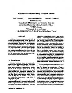
TIRAMOLA Decision Making User policies

II. R ELATED W ORK

Monitoring Collect Metrics

Users

The work in [13] presents a resource manager that dynamically consolidates remote cloud resources based on predefined policies and a prototype for extending Torque clusters. Similarly in [14], the amount of servers in a data center is regulated in order to optimize energy consumption. The works in [15]–[17] solve the problem of optimizing the resources of each VM (CPU, memory, etc) to achieve maximum performance, while the work in [18] aims at minimizing cost and maximizing throughput via training sessions and linear programming. These works do not address NoSQL systems and their performance under dynamic cluster resizes. Instead, we utilize multi-grained monitoring that uses a rich set of metrics to realize any resize policy. The work in [19] presents policies for elastically scaling a Hadoop-based storage tier based on automated control. CPU utilization dictates the number of VMs needed to satisfy a pre-defined objective (e.g., response time should be less than 3 sec). This approach is HDFS-specific using integrated monitoring; our framework is able to optimize resource allocation based on a rich set of user-defined policies and collected metrics. The work in [20] allows customization of applicationinternal modules such as the consistency protocol, routing (e.g., master-slave vs. DHT) and load balancing. Nevertheless, it does not elastically scale committed resources. In [21], users supply hints about the nature of the application, allowing the framework to modify its scheduling policies to improve application performance. The difference is the need for a middleware to be installed inside the cloud management layer, whereas we only utilize cloud client tools, being completely agnostic about the internals of the cloud management platform. A flexible language for controlling multi-dimensional elastic properties is defined in [22]. The approach in [23] is similar to our decision making module, with an effort to designate a suitable number of virtual machines in order to maximize profit. The system takes into consideration high-level metrics (e.g., application response time) and employs microeconomics to converge to a proportional sharing equilibrium. Our approach is far more general, as it can employ any cost or optimization model to its functionality. CloudWatch [8] provides VM-based metrics which, in combination with AutoScaling [24], allow simple policy descriptions that trigger resize actions. Yet, the metric support is limited to hypervisor-related information. CloudWatch is a general purpose tool that requires extra coding to reconfigure a NoSQL cluster after a resize operation. This is also the case for other frameworks such as [25], [26]. Solutions in this category put the burden of the decision and the amount of committed or freed resources solely to the users, while sometimes resulting in expensive vendor lock-ins (e.g., [9]).

Get fresh metrics

Load

Fig. 1.

Resize Action Orchestrate Cluster Cluster Coordinator

Cloud Management Adjust resources

Manage Add/delete NoSQL nodes VMs

Virtual NoSQL Cluster

Cloud Provider

Architecture of the TIRAMOLA elasticity-provisioning framework.

III. A RCHITECTURE TIRAMOLA [27], [28] is an open-source project that delivers automatic resource allocation for NoSQL clusters. It features a modular architecture illustrated in Fig. 1. The Decision Making module incorporates both the user-policy defined through an optimization function as well as cluster- and client-side monitored metrics and periodically decides on cluster resize actions. It outputs resize actions to the Cloud Management module that interacts with the cloud vendor in order to release or acquire more virtual machines. The Cluster Coordinator is then responsible for orchestrating the addition and removal commands relative to the particular NoSQL cluster in hand. The Monitoring module maintains up-to-date performance metrics collected from both cluster nodes and client nodes. Below we describe each module in more detail: Decision Making Module: This module is responsible for deciding the appropriate cluster resize action according to the applied load, cluster and user-perceived performance and optimization policy. TIRAMOLA formulates this process as a Markov Decision Process (MDP) that continuously identifies the most beneficial action relative to the current system state. The user goals are defined through a reward function that translates the optimization each application wishes to adhere to. Upon reaching a resize decision, the module forwards this command to the Cloud Management module. Monitoring: TIRAMOLA uses Ganglia [29], a scalable distributed monitoring tool that allows remote collection of live or historical cluster statistics (such as CPU load averages, network, memory or disk space utilization, number of open client threads, etc) through its XML API. Apart from the server-side metrics, modifications have been performed that allow Ganglia to collect user-related metrics. This is necessary, since the system state may also depend on user-related information such as mean query latency. To achieve this, we have modified our clients so that each one reports its own metrics by utilizing a well-known Ganglia operation called gmetric spoofing. With this mechanism, the monitoring module feeds the decision making module with an up-to-date system state, taking into account both client and server side metrics.

Cloud management: Our system interacts with the cloud vendor using the well known euca2ools, an Amazon EC2 compliant REST-based client library. This module receives as input commands for a NoSQL cluster resize (in the number of running VMs). Our cloud management platform is a private OpenStack [6] installation. The use of euca2ools along with the creation of Amazon Machine Images (AMIs) with preinstalled versions of the supported NoSQL systems and Ganglia guarantees that TIRAMOLA can be deployed in practically any EC2-compliant IaaS cloud. Cluster coordinator: The orchestration of newly commissioned or freed resources from the NoSQL cluster is performed with the remote execution of shell scripts and the injection of automatically created NoSQL-specific configuration files to each VM. A high-level “start cluster”, “add NoSQL node(s)” and “remove NoSQL node(s)” command is thus translated to a workflow of the aforementioned primitives. Our implementation ensured that each step has succeeded before moving to the next one, using applicable time-outs. Our framework has successfully incorporated three popular NoSQL systems that exhibit elastic behavior: HBase (see experimental evaluation), Cassandra and Riak. The system is extensible enough to include more engines that support elastic operations by implementing the system’s abstract primitives in the Cluster Coordinator module and by including the system’s binaries to the existing AMI virtual machine image. The precooked virtual machine image is available for download from the project’s web site. TIRAMOLA also strives to be robust: It periodically checkpoints and can be restarted after a failure; required state is maintained through the monitoring module as well as the underlying IaaS platform. A. Decision Making as an MDP Reinforcement Learning [30] is defined as the task of learning how to behave in a certain environment. A Markov Decision Process (MDP) [31] is defined by the tuple (S, A, {Psas0 }, γ, Rsas0 ), where S is a set of states, A is a set of actions, {Psas0 } = P r{st+1 = s0 |st = s, at = a} is a set of transition probabilities, γ ∈ [0, 1) is the discount factor and Rsas0 is a reward function. At each time step t, the system finds itself in state s. Choosing action a ∈ A at the current state brings the agent to the next state s0 with probability Psas0 , receiving a reward of Rsas0 . The total reward (or return) is given by the discounted sum of rewards. For finite MDPs, an optimal action per state solution exists; it is equivalent to computing the optimal action-value functions Q∗ (s, a), defined as the expected return when the agent starts from that state and takes action a. Action-value functions satisfy the Bellman optimality equation [30]. TIRAMOLA formulates resize decisions as an MDP that continuously identifies the most beneficial action. Benefits (both short and long-term) are defined through a reward function that translates the optimization/cost-model each application adheres to. First, we ensure that the Markov property holds for this formulation. Indeed, each of the module’s decisions are made regardless of how the cluster population

has been assembled so far, but only depends on the current state (i.e., number of VMs, CPU, memory, etc) and the action it perceives will be most beneficial. The tuple that describes our MDP (S, A, P, γ, r) is formulated as follows: States S = {S1 , S2 , ..., SM }, where Si represents a cluster with i ∈ [1, M ] NoSQL worker nodes (VMs) up and running. Actions A(s): Available actions are to add-, remove-node, or do nothing (no-op). The action space may also be quantified by allowing only certain number(s) of VM instances to be added or deleted (e.g., add_2, add_4 and remove_2, remove_4, etc). The transition probability matrix P : paij is the probability of transitioning from state i to state j given that action a was a taken. For our setting: paij = 1 if permissible i − → j and 0 otherwise. A transition is permissible if adding (removing) VMs results in the exact number of VMs being added (subtracted) to the initial cluster, or after a no-op the state remains the same. The model can be generalized to include the possibility of a partially successful permissible operation, i.e., paij = f, 0 ≤ f ≤ 1 (e.g., adding 4 nodes may result in only increasing cluster size by 2). Reward function r(s): It represents a numerical level of “goodness” of being at state s. This is an important part of the formulation, as reward maximization by the module leads to different optimal policies using different reward functions. In general, r(s) = ϕ(gains, costs), i.e., a policy is defined by appropriately incorporating various measurable or verifiable quantities into the reward function. For example, high throughput or served query rate can be profitable while query latency that violates an SLA, the costs per VM, etc can be considered costly. Finally, the discount factor 0 ≤ γ < 1 accounts for both present and future rewards. This formulation allows for a large degree of freedom: First, the finite MDP allows for optimal solution regardless of our knowledge of the environment or its dynamics: the system may learn directly from experience without a model of the environment’s dynamics. Second, the learning is realtime and continues through the entire life of the system. The module learns and acts simultaneously, reacting to changes in the rewards, the environment, etc. Third, the definition of the reward function leads to different optimization goals by different providers. B. Real-time Decision Making Given the values for Q∗ , greedily choosing any action that maximizes Q∗ (s, a) for any state s is proved to provide optimal behavior [30]. Solving Bellman’s equations for the exact Q∗ (s, a) values requires solving a system of linear equations, which is akin to an exhaustive search, looking ahead at all possibilities. Besides the computational expense, this is unrealistic in terms of exact knowledge of the system and application dynamics. Instead, TIRAMOLA uses Q-learning [30] to compute the optimal action-state values which updates Q(s, a) at each time a decision is made: Q(s, a) = Q(s, a) + α[r(s0 ) + γ max Q(s0 , a0 ) − Q(s, a)](1) 0 a

#VM=v1

#VM=c

#VM=v2

Latency

Latv2

Latency

Latc

Latency Latv1

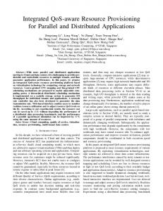
exhibits latency Latc with incoming load equal to λc . In order to compute r(v1) and r(v2) we cluster the data points inside the grey areas (the corresponding λ-slices) and choose the centroids’ y-coordinates (Latv1 , Latv2 ). In general, we elect representative points over p datasets of (d − 1) dimensions, where p is the number of permissible transitions from the λc λ λ λ current state. For each such dataset, only the data points that Fig. 2. Example of choosing the appropriate latency values in order to reside inside a (d − 1)-hypercube are fed to the clustering compute r(s) = ϕ(latency, VMs) engine. Our MDP approach has the advantage that it does not where 0 < α ≤ 1 is the learning rate. Q values are stored in require a model of the environment while it is naturally a look-up table and updated using (1). After each transition implemented in an online, fully incremental fashion with a from the previous state s to the current state s0 , an incremental minimal amount of computation. Training is important in adjustment is made to the estimated value of the previous the initial execution phases to ensure correct behavior with state-action pair Q(s, a). With the learning rate decaying to minimal (or no) experience. As time progresses and Q values zero asymptotically and Q(s, a) values represented using a are refined, real-time monitoring statistics prevail and are used lookup table, (1) is guaranteed to converge to the optimal by (1) to estimate action-state values. Finally, it is important to value function Q∗ (s, a), provided that the policy for action note that this formulation allows real-time policy learning and selection is asymptotically greedy, i.e., it chooses the action adaptation: Changing the way the Decision-Making module with highest Q-value in a given state. acts because an application has different requirements or TIRAMOLA utilizes training sessions in order to speed up (more rarely so) because the VM/cluster properties change convergence and increase the accuracy of estimating r(s). This is as simple as changing the reward function r or resetting is important in order to produce a realistic and accurate greedy the Q values. The latter is necessary for example when the policy, especially in the first stages of the learning process. infrastructure serving the cluster changes drastically. In TIRAMOLA, we implement an incremental, online method IV. E XPERIMENTAL R ESULTS executed inside the Decision Making module to estimate r(s) values described below: The experimental section intends to showcase the appliData collected from the monitoring module form a d- cability of TIRAMOLA as a control and monitoring layer dimensional dataset, with d >= 2. The dimensions that that manages a NoSQL cluster over an IaaS provider. Our participate de facto are the rate of incoming load λ and the size evaluation plans to demonstrate the following: (1) automatic of the cluster (number of VMs). Each metric that participates management of VM resources under incoming loads of difin the reward function is further added to the dimensions of ferent amplitude and frequency, (2) adaptation relative to our model. As the cluster operates, a d-dimensional table is different reward functions supplied and (3) sensitivity towards enriched with one point at each polled interval. When the the training phase and the amount of permissible states. time for a decision comes, the system must compute r(s0 ) for each state s0 that we are permitted to go to from the A. Experimental Setup current state s. Our method is based on the rationale that the system acts in a predictable manner, behaving similarly under similar conditions. Thus, we perform a clustering of the (d − 1)-dimensional datasets (excluding the dimension about the number of VMs) that correspond to states {s0 }. Yet, not all the data points are included: Following our rationale, we are interested in measurements relative to the current cluster load. Thus, and to account for some degree of variability, we only allow the points within a certain “slice” of λ values around the current load measurement to be fed to the clustering engine. The centroid of the largest cluster (if the number of clusters k > 1) can then be used as a representative point whose coordinates will be used to compute r(s0 ). Fig. 2 gives an example of this process. We assume that r(s) = ϕ(latency, VMs). The three graphs represent three 2-dimensional datasets, one for each different cluster size, namely v1, v2, and c (the current cluster size), with v1 < c < v2. All data-points collected so far are marked with an ‘x’. When the system decides for a possible resize, the most recent measurement is marked with a blue ‘x’, meaning the cluster

Our experimental setup consists of an OpenStack cactus private cluster [6] of 20 client VMs (load generators) and 16 server VMs. Each server VM has a 4 virtual core processor with 8GB of RAM and 50GB of storage space, while client VMs have 2 virtual cores and 4GB of RAM. The versions of Hadoop and Ganglia used are 1.0.1 and 3.1.2 respectively, both in their default configuration. We utilize an HBase (v. 0.92.0) cluster with initial size of 4 VMs (can be increased up to 16 VMs and downsized to a single VM – excluding the HMaster). The cluster is loaded using the well-known YCSB benchmark [32] with 20M records. HBase is configured with a replication factor of 3. Our workload is also created through the YCSB tool. Loads comprise simple get queries (UNIFORM READ query types). In [4] we present results showing how different NoSQL engines behave relative to different load types, namely zipfian random reads, uniform random updates and uniform random read-modify-writes. We also take into account the seasonal effect of web serving applications, in which load increases during peak hours and drops during non-peak hours. For

400

600

0

800

200

600

0

800

200K

20 16

150K

12

100K

8 50K

4

Fig. 4.

Cluster Size

Cluster Size

4

0

200

400

600

8

4

0

800

0

200

400

600

0

800

Time (min)

600

800

0

20 16

150K

50K

4

200

400

600

800

0

50K

4

0

For each policy, the system behaves in different ways, as different states are viewed more favorable based on the respective cost function. The A, B, C parameters are calcu-

16 12

200

400

600

800

8 50K

0

Time (min)

System behavior when applying four loads with frequency

r1 (s) = −C · |V M s|, r2 (s) = B · thr, r3 (s) = B · thr − C · |V M s|2 , r4 (s) = B · thr − C · |V M s| − A · lat

150K

20

100K

8

Time (min)

instance, Akamai’s 24-day load (Fig. 14 in [33]) and Microsoft Messenger’s weekly load (Fig. 5 in [34]) present a similar pattern (load consistently increases and decreases). To assist the decision making module into the estimation of the r(s) values (Section III-B), we apply a training phase. Our default training set is a simple sinusoid-like load with an average value around 70K req/sec, a peak of over 130K req/sec and a period of about 300 minutes. For the clustering component, we use a centroid-based method [35] with k = 3, choosing the centroid of the largest cluster inside a 4K req/sec (d − 1)-hypercube slice. In our experiments, a value for k around 2–4 manages to effectively prevent outliers in the decision process. In the future, we plan to incorporate a load prediction module that will allow a more accurate estimate of the λ-slice. Monitoring collects a new data point every minute and the decision daemon is invoked every 10 minutes. The resized cluster size is roughly available after 5 minutes, due to VM initialization and setup steps. For system robustness and to avoid oscillations, we set a backoff period of 5 minutes (10 minutes if a removal was decided) before a new resize operation is possible. Finally, we note that we do not consider data inconsistency issues caused, for example, by a simultaneous removal of all object replicas when removing more than 2 VMs (with a replication factor of 3). In large, production-level systems, this can be handled by either limiting the number of concurrent removals, or maintaining a baseline number of VMs under which the cluster size is not allowed to fall. We devise four different reward functions: function r1 (s) considers only VM costs, function r2 (s) considers only throughput gains, r3 (s) considers throughput and increased (squared) costs per VM, while r4 (s) considers all available metrics, throughput, latency and VM costs:

200K

12

100K

8

0

200K

Cluster Size

Load (req/sec)

12

100K

400

12

50K

Time (min)

Cluster Size Load (req/sec)

16

150K

Time (min)

16

System behavior when applying four loads of different amplitude (1K, 10K, 45K and 70K req/sec) using r4 (s) 20

200

8

Time (min)

200K

0

400

150K

100K

50K

4

Time (min)

Fig. 3.

12

100K

8

0

16

Cluster Size Load (req/sec)

200

150K

Cluster Size Load (req/sec)

0

12

100K

50K

4

16

20

Load (req/sec)

8 50K

Cluster Size

12

100K

150K

Load (req/sec)

Cluster Size

16

Load (req/sec)

Load (req/sec)

150K

20 200K

20 200K

200K

20

200K

1 ×, 2

0

4

200

400

600

800

0

Time (min)

2×, 4× and 10× of the training dataset using r4 (s)

lated using our experience with the HBase cluster to ensure stability under common workloads (our chosen values are A = .001, B = .001, C = .5). We note here that it is not our intent to identify the optimal reward function: Our goal is to demonstrate the system’s flexibility to use virtually any reward function according to the vendor or application policy. We leave fine-grained reward function modeling for future work. Nevertheless, since TIRAMOLA is open-sourced and functions are defined by editing a simple configuration file, anyone can freely download, modify and integrate it with their current infrastructure. B. Changing the incoming Load In our first experiment, we apply four loads of different amplitude with an average of 70K req/sec and register this input as well as the decisions taken using r4 (s) over time in Fig. 3. Solid lines depict the applied workload in req/sec whereas dotted lines represent the cluster size in number of VMs. The first three loads have approximate amplitudes of 1K, 10K and 45K req/sec. The fourth load has an amplitude of 70K req/sec with an average load of 120K req/sec. We notice how TIRAMOLA manages to behave according to the input load. When the load variation is small, only one decision is taken, moving the cluster from 4 to 9 VMs to optimize the received rewards. Since load does not significantly vary, gains are pretty stable, hence no other resize takes place. As incoming loads increase in amplitude, both increase and decrease size actions are taken. Cluster sizes change with frequency equal to the load frequency between 9–10 and 3–14 VMs respectively in the next two graphs. More resources are committed when bigger loads are applied and a bigger cluster downsize takes place respectively. The fourth graph showcases adaptation not only to bigger variability but also to states not seen before (through previous experience). Indeed, even though the training set allowed the collection of metrics for loads up to 140K req/sec, the applied load almost reaches 200K req/sec. Yet, the system is able to understand that committing all available VMs is necessary. Moreover, since

100K

8 50K

50K

4

800

200

600

800

4

200

16 12

150K

16 12

100K

8 4

600

800

600

0

0

800

4

200

400

600

0

800

Time (min)

0

50K

0

150K

20 200K

20

16

16

150K

12

100K

8

Time (min)

Fig. 6.

400

20 200K

Cluster Size

20 200K

100K

50K

12

System behavior under different reward functions, r1 (s), r2 (s), r3 (s) and r4 (s) respectively Cluster Size

Load (req/sec)

150K

400

0

16

8 50K

Time (min)

Load (req/sec)

Fig. 5.

200

8 50K

0

150K

100K

Time (min)

200K

0

400

12

4

200

400

600

800

Time (min)

0

8 50K

50K

0

12

100K

8

4

4

200

400

600

800

0

0

Cluster Size

600

8 4

Time (min)

16

100K

Cluster Size

400

0

150K

Load (req/sec)

200

0

12

Load (req/sec)

0

Cluster Size

100K

150K

20

Cluster Size

16

12

Cluster Size

16

20 200K

Load (req/sec)

20 200K

Load (req/sec)

Cluster Size

Load (req/sec)

150K

20 200K

Load (req/sec)

200K

200

Time (min)

400

600

800

0

Time (min)

Allowing to add/remove up to 1 and 8 nodes respectively at a 1× and 4× faster load using r4 (s)

the minimum load is over 50K req/sec, the minimum number of VMs is adequately set to 8. Fig. 4 shows how TIRAMOLA handles slower or faster load changes, with results for a load that changes twice as slow and 2, 4 and 10 times as fast. The rest of the parameters are kept the same as in the previous experiment. For the slower load, we notice that our system is able to provide extremely detailed resize actions adding and removing 1, 2 or 4 VMs at a time. As a consequence, the larger the period of a load, the more finegrained the decisions can be. Load changes at a slower rate than the module is allowed to decide. Yet, this is not true for the three remaining cases. TIRAMOLA is still able to adjust, following rates even 10 times faster than the training set at a decreasing granularity. Changes in the load occur so fast that the decisions dictate for increasingly larger VM additions and removals, until, as seen in the last graph, decisions are all about adding/removing 9–10 VMs per operation. In general, there exist several factors that affect the speed and granularity of adaptation: the rate at which the module is allowed to make decisions, the time required for these actions to be enforced and the actions available at each state. It takes both system- and application-specific parameter calibration to achieve a robust behavior in the majority of cases. In our experience, the realistic tests carried out on a relatively small sized cluster identify that the biggest limitation – assuming adequate training – is the VM request/allocation/initialization overheads. C. Changing the Reward Functions TIRAMOLA has the advantage of changing its resource allocation plan according to the defined policy: Different reward functions lead to different policies and business model optimizations. Fig. 5 shows the results of applying the four reward functions of Section IV-A using the training load of Section IV-B. When only the VM cost is taken into account (r1 (s)), the system is forced to always move toward the least number of nodes, regardless of load. Function r2 (s) produces almost

the opposite effect: Since throughput is the only metric of interest, the system moves to a state that maximizes it. The module does not decide for a resize as 14 VMs are adequate (for the incoming load) to provide maximum throughput for all applied amplitudes. The last two graphs display a system that automatically contracts and expands according to demand, since r3 (s) and r4 (s) take both gains and costs into account. Nevertheless, since VM costs are higher in r3 (s), the decisions are more conservative, ranging between 1 and 7 nodes. Using r4 (s) allows the cluster size to range from 2 to 14 nodes with resize moves that correspond directly to the changes in load. D. Changing the Action and Training sets So far, we have assumed that resize actions of any size are possible. Yet, our framework allows for customization of available actions. Actions of small granularity (e.g., 1–2 nodes) may not be adequate to optimize cluster performance when loads change abruptly; actions of larger granularity (e.g., allowing up to 8 concurrent node additions/removals at once) perform more radical changes at the risk of partially failing. Utilizing the training set and load of the previous experiments, we vary the number of maximum nodes that can be added/removed at a single action. For instance, using a maximum of 4 nodes allows the addition/removal of 1, 2, 3, or 4 nodes at a time. Fig. 6 shows the results under the default load and one changing four times as fast using r4 (s). The graphs clearly demonstrate the trend we described: When only a single node is allowed to change, cluster resizes come at a fine-grained manner, but, due to the inherent system delay, they cannot fully observe load variations. As more actions are allowed, the situation noticeably improves. For the faster changing load, our observations become more acute. Altering the cluster size by one node substantially fails to capture the changes in load, as our cluster moves between 11–13 VMs. While resize actions take place with the periodicity of the load, they are too small to allow for a proper contraction. Allowing larger resizes enables the cluster to shape its behavior (albeit at steeper notches)

16

150K

12

100K

100K

8

8

200

400

600

800

0

200

400

600

800

0

Time (min)

Time (min)

Fig. 7. 24 20 16 12 8 4 0

4

4 0

16

150K

12 8 50K

0

200K

150K

20 16 12

100K

100K

50K

50K

0

12

20

Cluster Size

16

200K

Cluster Size Load (req/sec)

20

Cluster Size Load (req/sec)

Cluster Size

Load (req/sec)

150K

20 200K

Load (req/sec)

200K

4

200

400

600

800

0

Time (min)

8 50K

0

4

200

400

600

800

0

Time (min)

Performance with min training and full training using T1, T2 and r4 (s)

3 10 MSQE 2.5 MSQE MSQE MAE 8 MAE MAE 2 6 1.5 4 1 2 0.5 0 2 4 6 8 10 12 14 16 0 100 200 300 2 4 8 10 6 max #VMs per resize #train.points per cluster size Load to training set freq. ratio

Fig. 8. Mean Absolute and Mean Square Error under varying input load frequency, resize actions and training points, using r4 (s)

relative to the incoming load. To measure the impact of training to the performance of TIRAMOLA, we vary the number of training points before a challenging load is applied to the system. Specifically, we apply a sinusoid-like load of 80K req/sec average rate and 60K req/sec amplitude with half the periodicity of the training set. We utilize two training sets, T1 and T2: T1 has an average around 60K req/sec and an amplitude of 45K req/sec (closer to the applied load with a difference in peak of about 35K req/sec), while T2 has an average around 40K req/sec and an amplitude of 20K req/sec (more challenging, up to 80K req/sec difference). For both training sets, we take two extreme cases, namely full training (i.e., a total of 5600 points over a 350 min period) and min training (i.e., a total of only 32 points collected). Results are shown in Fig. 7. When using T1 (first 2 graphs), the system is generally able to quickly assume the required periodicity regardless of the size of the collected experience. Yet, min training takes over 100 minutes to do so, while this happens immediately for full training. A striking difference is the amount of adaptivity to the load amplitude (compared to the training set): Min training has trouble choosing more than 12 nodes, while more informed training allows the system to reach 15. These findings are more evident in the case of training set T2 (last 2 graphs): The system gradually learns more appropriate states using realtime experience; the difference between more and almost no training is the learning rate: Full training reaches a 12-node cluster while min training achieves an increase from 4 to 9 nodes. From our findings, we deduce that both the amount as well as the quality of training experience affects performance. The larger the experience and closer it is to the real load, the faster the convergence to optimal resource management. Yet, the system is able to learn and move to the correct states as time and more real data points are collected. For a longrunning production cluster this effect is even less significant: Training and real-time experience is never reset (like in all the experiments presented in this work), adding up to the required knowledge for an informed decision by the system. To measure how close the system is to an “optimal” policy,

we re-consider all decisions after the end of each experiment, assuming full monitoring knowledge (based even on measurements that were not present at the time) and an unlimited set of actions available. For each decision c ∈ [1, 16] denoting the decided cluster size, we compute the optimal cluster size c∗ and the Mean Absolute Error (MAE) Pand Mean Squared Error (MSQE) quantities: MAE= n−1 1≤i≤n |ci − c∗i | and P MSQE= n−1 1≤i≤n (ci − c∗i )2 ,where n is the total number of resize actions. These metrics approach zero as decisions move close to the optimal ones. MAE, in particular, indicates the average difference (in number of VMs) of the clusters created through consecutive decisions from the optimal ones. Fig. 8 demonstrates that TIRAMOLA is robust and behaves very closely to an optimal decision maker. The first graph shows that increasing the number of allowed operations brings the allocation policy close to optimal: Allowing 4 or more VM resizes causes an average error of less than one VM per operation. After that point the algorithm is very close to the optimal policy. The second graph indicates that our method is extremely robust to loads even 10× faster than the training set. Finally, the third graph shows that increasing the number of training points per cluster configuration also improves performance. After just 100 points, our system takes actions less than one VM different to the optimal ones, a feature combined with learning of unseen loads (see Fig. 7). V. C ONCLUSIONS – D ISCUSSION This work presented TIRAMOLA, a fully modular, cloudenabled, open-source framework that can adaptively resize NoSQL clusters according to user-defined policies and incoming load. Our system allows seamless interaction with most IaaS platforms, requesting/releasing VM resources and orchestrating them inside a NoSQL cluster. It also features a monitoring module that reports both client and server side metrics in a scalable and efficient way. Resize decisions are modeled as a Markov Decision Process that automatically decides the most advantageous state to move the cluster to in real-time according to user- or application-defined policies. The system is very customizable, allowing different NoSQL engines, optimization strategies, permissible actions, input and training loads and, finally, varying degree of adaptation. To the best of our knowledge, this is the first open-source attempt to provide a cloud-based system for automatic VM provisioning for NoSQL clusters. This work spans a broad set of topics; we briefly discuss (due to lack of space) some important related issues here: Scalability: Such issues relate to both storage- and compute-

intensive operations carried out by the decision-making module. In the first case, we use a look-up table store for Q values; given that the permissible actions are bounded (e.g., add/remove b VMs, b