Jul 26, 2011 - We carefully designed and conducted a human survey to compare ... Keywords: text summarization, high-dimensional analysis, sparse mod-.
What is in the news on a subject: automatic and sparse summarization of large document corpora Luke Miratrix1∗ Jinzhu Jia2∗ Brian Gawalt3 Bin Yu1,3 Laurent El Ghaoui3 1 Department
of Statistics, UC Berkeley, Berkeley, CA 94720 of Mathematical Sciences and Center for Statistical Science, Peking University, Beijing, China, 100871 3 Department of EECS, UC Berkeley, Berkeley, CA 94720
2 School
July 26, 2011 Abstract News media play a significant role in our political and daily lives. The traditional approach in media analysis to news summarization is labor intensive. As the amount of news data grows rapidly, the need is acute for automatic and scalable methods to aid media analysis researchers so that they could screen corpora of news articles very quickly before detailed reading. In this paper we propose a general framework for subject-specific summarization of document corpora with news articles as a special case. We use the state-of-the art scalable and sparse statistical predictive framework to generate a list of short words/phrases as a summary of a subject. In particular, for a particular subject of interest (e.g., China), we first create a list of words/phrases to represent this subject (e.g., China, Chinas, and Chinese) and then create automatic labels for each document depending on the appearance pattern of this list in the document. The predictor vector is then high dimensional and contains counts of the rest of the words/phrases in the documents excluding phrases overlapping the subject list. Moreover, we consider several preprocessing schemes, including document unit choice, labeling scheme, tf-idf representation and L2 normalization, to prepare the text data before applying the sparse predictive framework. We examined four different scalable feature selection methods for summary list generation: phrase Co-occurrence, phrase correlation, L1-regularized logistic regression (L1LR), and L1-regularized linear regression (Lasso). We carefully designed and conducted a human survey to compare the different summarizers with human understanding based on news * Miratrix and Jia are co-first authors.
1
articles from the New York Times international section in 2009. There are three main findings: first the Lasso is the best overall choice of feature selection method; second, the tf-idf representation is a strong choice of vector space, but only for longer units of text such as articles in newspapers; and third, the L2 normalization is the best for shorter units of text such as paragraphs.
Keywords: text summarization, high-dimensional analysis, sparse modeling, Lasso, L1 regularized logistic regression, co-occurrence, tf-idf, L2 normalization.
1
Introduction
Joseph Pulitzer wrote in his last will and testament, “[Journalism] is a noble profession and one of unequaled importance for its influence upon the minds and morals of the people.” Faced with an overwhelming amount of world news, concerned citizens, media analysts and decision-makers alike would greatly benefit from scalable, efficient methods that extract compact summaries of how subjects of interest are covered in text corpora. These compact summaries could be used by the interested people for screening corpora of news articles before detailed reading or further investigation. We propose a novel approach to perform automatic, subject-specific summarization of news articles that applies to general text corpora. Our approach allows researchers to easily and quickly explore large volumes of news articles. These methods readily generalize to other types of documents. For example, El Ghaoui et al. (2011) identified potentially dangerous aspects of specific airports by using these methods on pilots’ flight logs. We are currently implementing our approach within an on-line toolkit, SnapDragon,1 which will soon be available to researchers interested in screening corpora of documents relative to a subject matter. News media significantly drives the course of world events. By choosing which events to report and the manner in which to report them, the media affects the sentiments of readers and through them the wider world. Exposure to news can drive change in society (Miller and Krosnick, 2000; Nisbet and Myers, 2010; Hopkins and King, 2010), and, even when controlling for topic, can vary in tone, emphasis, and style (Branton and Dunaway, 2009; Gilens and Hertzman, 2000; D’Alessio and Allen, 2000). Our focus on news media is motivated by a crucial need in a democracy: to understand precisely where and how these media variations occur. 1
http://statnews2.eecs.berkeley.edu/snapdragon
2
Currently, media analysis is often conducted by hand coding (Wahl et al., 2002; Denham, 2004; Potter, 2009). Hand-coding manually reduces complex text-data to a handful of quantitative variables, allowing for statistical analysis such as regression or simple tests of difference. It is prohibitively laborintensive (Hopkins and King, 2010). In personal correspondence, Denham relayed that each article took roughly fifteen minutes to analyze, suggesting about 28 hours of time for their full text corpus of 115 articles. In the last five years we have seen the emergence of a computational social science field connecting statistics and machine learning to anthropology, sociology, public policy, and more (Lazer et al., 2009). Many organizations have introduced automated summary methods: Google news trends, Twitter’s trending queries, Crimson Hexagon’s brand analysis and others all use computation to make sense of the vast volumes of text now publicly generated. These approaches, discussed below, illustrate the potential of computation for news media analysis. Summarization by extraction. There are two major approaches to text analysis, key-phrase extraction (listing key-phrases for the document such as in Rose et al. (2010); Senellart and Blondel (2008); Frank et al. (1999); Chen et al. (2006)) and sentence extraction (identifying and presenting the “most relevant” sentences of a document as a summary, such as in Hennig (2009); Goldstein et al. (2000); Neto et al. (2002)). Both these approaches score potential key-phrases or sentences found in the text and then select the highest scorers as the summary. This line of research has primarily focused on summarizing individual documents, with one summary for every document in a corpus. However, when there are multiple documents, even a short summary of each document adds up quickly. Content can be buried in a sea of summaries if most documents are not directly related to the subject of interest. If many documents are similar, the collection of summaries becomes redundant. Moreover, if the subject of interest is usually mentioned in a secondary capacity, it might be missing entirely from the summaries. To address some of these problems, Goldstein et al. (2000) worked on summarizing multiple documents at once to remove redundancy. Under their system, sentences are scored and selected sequentially, with future sentences penalized by similarity to previously selected sentences. In this system, the documents need to be first clustered by overall topic. Hennig (2009) fits a latent topic model (similar to LDA, discussed below) for subject-specific summarization of documents. Here the subject is
3
represented as a set of documents and a short narrative of the desired content. All units of text are projected into a latent topic space that is learned from the data independent of the subject and then sentences are extracted by a scoring procedure by comparing the similarity of the latent representations of the sentences to the subject. Although we also summarize an entire collection of documents as they pertain to a specific subject of interest, we do not use a latent space representation of the data. In Monroe et al. (2008), the authors merge all text into two super-documents and then score individual words based on their differing rates of appearance, normalized by their overall frequency. We analyze the corpus through individual document units. Summarization via topic modeling. Some analysis algorithms take text information as input and produce a model, usually generative, fit to the data. The model itself captures structure in the data, and this structure can be viewed as a summary. A popular example is the latent Dirichlet allocation (Blei et al., 2003), which posits that each word observed in the text is standing in for a hidden, latent “topic” variable. These models are complex and dense, with all the words playing a role in all the topics, but one can still take the most prominent words in a topic as the summary. Chang et al. (2009) had humans evaluate the internal cohesion of learned topics. Respondents were asked to identify “impostor” words inserted into lists of words representing a topic. This showed these approaches as producing cogent and reasonable topics. Supervised versions (Blei and McAuliffe, 2008) of these methods can be used to summarize a subject of interest. Although these methods are computationally expensive and produce dense models requiring truncation for interpretability, they are powerful indications of the capabilities of computer-assisted summarization. These methods analyze the corpus as a whole and model how the documents cover a modest number of organically grown topics. We opt instead for a more directed process of summarizing a particular, specified subject (out of possible millions). Other automated approaches. Google Trend charts are calculated by comparing the number of times a subject appears in the news outlets that Google compiles to the overall volume of news for a specified time period. Even this simple approach can show how subjects enter and leave public discourse across time. Twitter’s trending topics appears to operate similarly, although it selects the hottest topics by those which are gaining in frequency
4
most quickly. Although neither of these tools summarize a specified subject, they are similar in spirit to the normalized simpler methods (co-occur and correlation screen) that we will introduce and investigate in this paper. Hopkins and King (2010)extrapolates from a potentially non-random sample of hand-coded documents to estimate the proportion of documents in several pre-defined categories. This can be used for sentiment analysis (e.g., estimating the proportion of blogs showing approval for some specified public figure). We instead identify key-phrases most associated with a given subject. These key-phrases could then be analyzed directly for sentiment, thus reducing the amount of hand-coding required. Their work is behind Crimson Hexagon, a company currently offering brand analysis to several companies. In a similar spirit, we believe there is opportunity to answer the question, “What is being said in the news regarding China?” or, more generally, “What is discussed in this corpus of documents regarding subject A?” using machine learning techniques. Our predictive and sparse approach with human evaluation. In this paper, we propose to use statistical machine learning tools such as Lasso that are fast, sparse, and different from those described earlier to produce short and interpretable summaries. Our proposal is desirable because media analysis (or general document summarization) tools need to encourage exploration, allowing researchers to easily examine how different topics are portrayed in a corpus or how this portrayal evolves over time or compares across different corpora. Given a corpus of documents (e.g., the New York Times International Section articles in 2009) as well as a subject of interest (e.g.,subject China as represented as a short list of words China, Chinas and Chinese), we establish the predictive framework by first automatically labeling documents into positive and negative examples by, for example, determining if they contain words from the subject list. Counts of words/phrases not on the subject list then form the predictor vectors for the documents. After normalizing these vectors, we use scalable, reproducible prediction and classification techniques to identify a small set of words and phrases that best predict the subject as it appears. This overall arc reduces corpora of many millions of words into a few representative key-phrases that constitute how the given subject is treated in the corpus. To validate these summaries we cannot use traditional machine learning approaches, however, since traditional measures have no guarantee of cor-
5
relating with actual meaning. We therefore compare the different summary approaches with a human survey. We find that sparse methods such as Lasso indeed produce higher quality summaries than many currently used, simpler, methods. Moreover, we conducted usability testing to investigate how different preprocessing techniques differ in quality of resulting lists in the user survey. We found the choice of preprocessing important, especially with simpler summarization methods. The sparse methods such as Lasso, however, are more robust to potential mistakes made in the data preparation step. To illustrate, consider how the New York Times treated China (represented as “china, chinas, chinese”) in the international section in 2009. One of our summary methods, L1LR, yields a short list of terms: “beijing, contributed research, global, hu jintao, imports, of xinjiang, peoples liberation army, shanghai, sichuan province, staterun, tibet, trade, uighurs, wen jiabao, xinhua news agency”. This succinct summary captures main relevant personalities (e.g., Wen Jiabao, Hu Jintao), associated countries and areas (e.g., Uighurs, Tibet), entities (Xinhua news), and topics (trade, imports, global [activity], state-run [organizations]). The presence of “contributed research” indicates that other people, in addition to the authors, contributed to many of the Times articles on China. These terms inform interested readers including China experts about how China is being treated by the New York Times and suggest directions for further reading on topics such as Sichuan, Xinjiang, Tibet, and trade. Table 2 contains four other sample summaries. The rest of the paper is organized as follows. Section 2.1 describes our proposal including the predictive framework and the preprocessing choices used in the study. Section 2.2 proposes different key-phrase selectors (e.g.,Lasso, co-occurrence) one might use to generate the final summary. We then describe the validation experiment designed to examine the performance of the summarizers built from the choices in Sections 3. Results of this experiment are shown in Section 4. Section 5 concludes.
2
Our approach: predictive, fast, and sparse
Our approach is based on a predictive binary classification framework. In a typical binary classification scenario, data units (e.g.,news articles or paragraphs) belong to two classes and features of a data unit are used to predict its class membership. Classification of text documents using the phrases in those documents as features is familiar and well-studied (Genkin et al.,
6
2007; Zhang and Oles, 2001). We turn subject-specific (e.g., China) summarization into a binary classification problem by forming two classes, that is, we automatically label news articles (or other document units) in a corpus as subject-related and irrelevant. See Section 2.1.3, where we discuss several different ways of labeling. We then use a predictive classifier to generate a summary list. To be precise, we take those words and phrases most important for classification as a summary of the subject relative to the corpus. A predictive framework consists of n units, each with a class label yi ∈ {−1, +1} and a collection of p possible features that can be used to predict this class label. Each unit i ∈ I ≡ {1, . . . , n} is attributed a value xij for each feature j ∈ J ≡ {1, . . . , p}. These xij form a n × p matrix X. The n units are blocks of text taken from the corpus (e.g., entire articles or individual paragraphs), the class labels yi indicate whether document unit i contains content on a subject of interest, and the features are all the possible key-phrases that could be used to summarize the subject. As mentioned earlier, we consider several ways of automatically labeling or assigning class memberships based on the document unit itself in Section 2.1.3. Matrix X and vector y can be built in several ways. We build X by reweighting the elements of a document-term matrix C: Definition A document-term matrix C sets Cij := The number of times key-phrase j appears in document i This is often called the bag-of-phrases model : each document is represented as a vector with the jth element being the total number of times that the specific phrase j appears in the document. Stack these row vectors to make the matrix C ∈ Rn×p of counts. C has one row for each document and one column for each phrase. C tends to be highly sparse: most entries are 0. To transform raw text into this vector space, convert it to a collection of individual text document units, establish a dictionary of possible phrases, and count how often each of the dictionary’s phrases appear in each of the document units. Once this is completed, the summarizing process consists of 3 major steps: 1. Reweight: build X from C; 2. Label: build y by identifying which document units in the corpus likely treat the specified subject; 3. Select: extract a list of phrases that ideally summarize the subject. 7
How the document units are labelled, how the document units are vectorized, and how phrases are selected can all be done in different ways. Different choices for these steps result in different summarizers, some better than others. We describe these steps and choices fully in Sections 2.1 and 2.2. Iraq american and afghanistan baghdad brigade combat gen in afghanistan invasion nuri pentagon saddam sergeant sunni troops war and who
Russia a medvedev caucasus europe gas georgia interfax news agency iran moscow nuclear president dmitri republics sergei soviet vladimir
Germany angela merkel berlin chancellor angela european france and frankfurt group of mostly hamburg marwa alsherbini matchfixing minister karltheodor zu munich nazi world war
Mexico and border protection antonio betancourt cancn chihuahua denise grady drug cartels guadalajara influenza oaxaca outbreak president felipe sinaloa swine texas tijuana
Table 1: Four Sample Summaries of Four Different Countries. The method used, a count rule with a threshold of 2, the Lasso for feature selection, and tf-idf reweighting of features, was one of the best identified for article-unit analysis by our validation experiment.
2.1
Data pre-processing
In this section, we describe in detail how we pre-process a corpus of documents into a vectorized space so that the predictive classification approach can be employed. Our description is for a general document corpus, but at times we use examples from news article summarization to ground the general description and to show the need to consider context.
8
2.1.1
Choosing the document units
We divide the raw text into units of analysis and determine which of those units have relevant information about the subject, and summarize based on common features found in these units. The granularity with which the text is partitioned may then have some impact on the resulting summaries. In particular, we hypothesized that using smaller, lower-word-count units of text should produce more detail-oriented summaries, while using larger units will highlight key-phrases dealing more with the larger themes discussed when the subject of interest is mentioned. We tested this hypothesis by comparing summarizers that analyze at the article level to those which analyze at the component-paragraphs level. Interestingly, we found no large differences. See Section 4.4. 2.1.2
Identifying potential summarizing phrases
To build the document-term matrix C we first identify all possible phrases that could be part of a summary. This list of possibilities constitute our dictionary. Building this dictionary begins with asking, “Which text phrases are acceptably descriptive?” Sometimes the answer to this question suggests a manually-defined dictionary: if summaries should only list, e.g., countries then the dictionary would be easy to assemble by hand. In many situations, however, the dictionary of terms should be kept large, and possibly be drawn from the corpus itself. Different decisions— Should capitalization matter? Are punctuation marks terms? Can terms include numerals?—yield dictionaries varying widely in size and utility. Terms could be further disambiguated by many natural language tools, e.g., part-ofspeech tagging, which would again increase dictionary size. Any automated system for forming a dictionary will entail at least some uncertainty in term identification. We elected to use a large dictionary containing all phrases of up to three words in length. We generated our dictionary by first removing all numerals and punctuation, then case-folding (converting all text to lowercase). We then segmented each document into overlapping phrases, consisting of all single words, bigrams and trigrams in that document unit. Some text analysts stem their phrases, reducing words to a core root prefix, e.g., truncating “terror,” “terrorist,” and “terrorism” to “terror”. But we do not stem. There is a semantic difference if a particular subject is associated with “canadians”, the citizenry versus “canada” the country. For our corpus of articles from the New York Times International Section in 2009,
9
this identified in 4.5 million distinct phrases. A first-pass pruning, removing all phrases appearing fewer than six times, resulted in a dictionary of p = 216, 626 distinct phrases. 2.1.3
Representing subjects as lists of words/phrases and automatically labeling documents
We train a classifier to predict document labels, yi ∈ {−1, +1}, with their vectors of phrase features, xi ∈ Rp , for i = 1, . . . , n. In the labeling step we automatically build the label vector y = (y1 , . . . , yn ) by deciding whether each document unit in the corpus should be considered a positive class example or a negative class example. Establishing the class labels for a news document corpus is sometimes straightforward. For instance, for comparing 1989 articles about mental illness to those from 1999 as Wahl et. al did, the labels would be simple: the documents from the opposing years go in opposite classes. We build y by identifying which of the document units treat the subject of interest with ”treat” being precisely defined later. For small enough n, y could be built by hand. For corpora too large to admit manual labeling, we need reasonable automatic labeling. Ideally this need not be a perfect identification—noise in labeling should not have undue impact on the resulting summaries. In the large sense, a subject is a concept of interest that an investigator might have. We represent a subject with a small list of words or phrases, e.g., the subject of China would be well represented by the set {“china,” “chinas,” “chinese”}. Specifically, let the subject Q ⊂ J be a list of words or phrases selected by the user to capture a subject of interest. count-m. We consider two general automatic labeling techniques. The first technique, count-m, marks document unit i as treating a subject if related phrases appear frequently enough, as given by: Definition Count-m labeling labels document unit i as: yi = 2 · 1{ri ≥ m} − 1 P where 1{·} is the indicator function and ri ≡ j∈Q cij is the total number of subject-specific phrases in unit i. hardcount-m. The second automatic labeling technique, hardcount-m, drops any document i with 0 < ri < m from the data set instead of labeling
10
it with −1. The hardcount method considers those documents too ambiguous to be useful as negative class examples. It produces the same positive example set as count-m. We hypothesized that dropping the ambiguous document units would heighten the contrast in content between the two classes, and thus lead to superior summaries. It did not. See Section 4.4. We generate y this way because we are interested in how a subject is treated in a corpus. Other approaches are possible. For example, y might identify which articles were written in a specific date range; this would then lead to a summary of what was covered in that date range. 2.1.4
Reweighting and removing features
It is well known that baseline word frequencies impact information retrieval methods, and so often raw counts are adjusted to account for commonality and rarity of terms (e.g., Monroe et al., 2008; Salton and Buckley, 1988). In the predictive framework, this adjustment is done in the construction of the feature matrix X. We consider three different constructions of X, all built on the bag-of-phrases representation. Salton and Buckley (1988) examined a variety of weighting approaches for document retrieval in a multi-factor experiment and found choice of approach to be quite important; we take a similar comparative approach for our task of summarizing a corpus of documents. We first remove the columns corresponding to the phrases in subject Q from the set of possible features J to prevent the summary from being trivial and circular. We also remove sub-phrases and super-phrases. For example, if Q is {“united states”} then candidate summary phrases “united”, “states”, “of the united”, and “states of america” would all be removed. The removal is easily automated. Our baseline then is to simply drop stop words (words determined a priori as too uninformative to merit inclusion). Our second approach is to rescale each phrase vector (column of C) to have unity L2 norm. Our third is an implementation of the tf-idf technique (Salton and Buckley, 1988; Salton, 1991), rescaling the bag-of-phrases components so that appearances of rarer phrases are considered more important than common ones. Stop Words. Stop words are low information words such as “and,” or “the”, typically appearing with high frequency. Stop words may be context dependent. For example, in US international news “united states” or “country” might be considered high frequency and low information. Highfrequency words have higher variance and effective weight in many methods, 11
causing them to be erroneously selected as features due to sample noise. To deal with these nuisance words, many text-processing methods use a fixed, hand-built stop-word list and preemptively remove all features on that list from consideration (e.g., Zhang and Oles, 2001; Ifrim et al., 2008; Genkin et al., 2007). This somewhat ad-hoc method does not adapt automatically to the individual character of a given corpus and presents many difficulties. Switching to a corpus of a different language would require new stop word lists. When considering phrases instead of single words, the stop word list is not naturally or easily extended. For example, simply dropping phrases containing any stop word is problematic: it would be a mistake to label “shock and awe” uninteresting. On the other hand, there are very common candidate phrases that are entirely made up of stop words, e.g., “of the,” so just culling the single word phrases is unlikely to be sufficient. See Monroe et al. (2008) for further critique. L2 -rescaling. As an alternative, appropriately adjusting the document vectors can act in lieu of a stop-word list by reducing the variance and weight of the high-frequency features. We use the corpus to estimate baseline appearance rates for each feature and then adjust the matrix C by a function of these rates; this core idea is discussed by Monroe et al. (2008). We define L2 -rescaling to be: Definition X is a L2 -rescaled version of C if each column of C is rescaled to have unit length under the L2 norm. I.e.: n
X cij xij = √ , where zj ≡ c2ij zj i=1
tf-idf Weighting. An alternate rescaling comes from the popular tf-idf heuristic (Salton, 1991), which attempts to de-emphasize commonly occurring terms while also trying to account for each document’s length. Definition X is a tf-idf weighted version of C if � � cij n xij := log qi dj P where qi ≡ Ppj=1 cij is the sum of the counts of all key-phrases in document i and dj ≡ ni=1 1{cij > 0} is the number of documents in which term j appears at least once. 12
Under tf-idf, words which appear in a large proportion of documents are shrunk considerably in their representation in X. Words which appear in all n documents, such as “the”, are zeroed out entirely. A potential advantage of tf-idf is that it might ease comparisons between documents of different lengths because term counts are rescaled by the total count of terms in the document. To illustrate the advantages of reweighting, we generated four summaries from the L1LR feature selection method with all combinations of L2 -rescaling and stop-word removal (see supplementary material). Without reweighting, if no stop words are deleted the list is dominated by highfrequency, low-content words such as “of,” “and,” and “was”. The just stop-word removal list is only a bit better. It contains generic words such as “mr,” “percent,” and “world.” The rescaled list does not contain these words. This is a common problem with stop-word lists: they get rid of the worst offenders, but do not solve the overall problem. The list from stopword removal together with L2 -rescaling and the list from just L2 -rescaling are the same—the rescaling, in this case, has rendered the stop-word list irrelevant. We hypothesized that feature weighting is more transparent and reproducible than stop-word removal and that it results in superior summaries when compared to stop-word removal. With the human validation experiment, we compared using L2 -rescaling, tf-idf weighting, and stop-word removal as the pre-processing step for each of our feature selectors and found that humans indeed prefer lists coming from the reweighting methods.
2.2
Four Feature Selection Methods
Classical prediction yields models that give each feature a non-zero weight. The models are thus hard to interpret when there are many features, as is typically the case with text analysis (our data set contains more than 200,000 potential phrases). We, however, want to ensure that the number of phrases selected is small so the researcher can easily read and consider the entire summary. Short summaries are quick to digest, and thus are easily comparable. Such summaries might even be automatically generated for a corpus in one language and then translated to another, thus easing comparison of media coverage from different nationalities and allowing insight into foreign language news (Dai et al., 2011). Fundamentally, a small set of features is more easily evaluated by human researchers. Given the features X and document labels y for a subject, we extract the columns of X that constitute the final summary. We seek a subset of 13
phrases K ⊆ J with cardinality as close as possible to, but no larger than, a target k, the desired summary length. We typically use k = 15 phrases, but 30 or 50 might also be desirable. The higher the value of k, the more detailed and complex the summary. We require the selected phrases be distinct meaning that we don’t count sub-phrases. For example, if “united states” and “united” are both selected, we drop “united”. The constraint of short summaries makes the summarization problem a sparse feature selection problem, as studied in, e.g., Forman (2003); Lee and Chen (2006); Yang and Pendersen (1997). Sparse methods, such as L1 penalized regression, naturally select a small subset of the available features (in our case candidate key-phrases) as being relevant predictors. In other domains, L1 -regularized methods are useful for sparse model selection; they can identify which of a large set of mostly irrelevant features are associated with some outcome. In our domain there is no reasonable underlying model that is indeed sparse; we expect different phrases to be more or less relevant, but few to be completely and utterly irrelevant. Nevertheless, we still employ the sparse methods to take advantage of their feature selection aspects, hoping that the most important features will be selected first. We examine four methods for extraction, detailed below. Two of them, Co-occurrence and Correlation Screening, are scoring schemes where each feature gets scored independently and the top-scoring features are taken as a summary. This is similar to traditional key-phrase extraction techniques and to other methods currently used to generate word clouds and other text visualizations. The other two (the Lasso and L1LR) are L1 regularized least squares linear regression and logistic regression, respectively. Table 2 displays four summaries for China, one from each feature selector: choice matters greatly. Co-occurrence and L1-penalized logistic regression (L1LR), are familiar schemes from previous work (Gawalt et al., 2010). 2.2.1
Co-occurrence
Co-occurrence is our simplest, baseline, method. The idea is to take those phrases that appear most often (or have greatest weight) in the positively marked text as the summary. This method is often used in, e.g., newspaper charts showing the trends of major words over a year (such as Google News Trends2 ) or word or tag clouds (created at sites such as Wordle3 ). 2 3
http://www.google.com/trends http://www.wordle.net/
14
1 2 3 4 5 6 7 8 9 10 11 12 13 14 15
Co-occurrence and by contributed research for global has hu jintao in beijing its of that the to xinhua year
Correlation beijing and beijings contributed research from beijing global in beijing li minister wen jiabao president hu jintao prime minister wen shanghai the beijing tibet xinhua the zhang
L1LR asian beijing contributed research euna lee global hong kong jintao north korea shanghai staterun uighurs wen jiabao xinhua
Lasso asian beijing contributed research exports global hong kong jintao north korea shanghai tibet uighurs wen jiabao xinhua
Table 2: Comparison of the Four Feature Selection Methods. Four sample summaries of news coverage of China. (Documents labeled via count-2 on articles, X from L2 -rescaling.) Note superior quality of Lasso and L1LR on the right.
By the feature selection step we have two labelled document subsets, I + = {i ∈ I|yi = +1}, of cardinality #I + , and I − = {i ∈ I|yi = −1}, of cardinality #I − . The relevance score sj of feature j for all j ∈ J is then: sj =
1 X xij #I + + i∈I
sj is the average weight of the phrase in the positively marked examples. For some k 0 , let s¯ be the (k 0 +1)th highest value found in the set {sj | j ∈ J }. Build K = {j ∈ J : sj > s¯}, the set of (up to) k 0 phrases with the highest average weight across the positive examples. Any phrases tied with the (k 0 +1)th highest value are dropped, sometimes giving a list shorter than k 0 . The size of K after subphrases are removed can be even less. Let the initial value of k 0 be k, the actual desired length. Now adjust k 0 upwards until just before the summary of distinct phrases is longer than k. We are then taking the k 0 ≥ k top phrases and removing the sub-phrases to produce k or fewer distinct phrases in the final summary. 15
If X = C, i.e. it is not weighted, then sj is the average number of times feature j appears in I + , and this method selects those phrases that appear most frequently in the positive examples. The weighting step may, however, reduce the Co-occurrence score for common words that appear frequently in both the positive and negative examples. This is especially true if, as is usually the case, there are many more negative examples than positive ones. Appropriate weighting can radically increase this method’s performance. 2.2.2
Correlation Screening
Correlation Screening selects features with the largest absolute correlation with the subject labeling y. It is a fast method that independently selects phrases that tend to appear in the positively marked text and not in the negatively marked text. Score each feature as: sj = |cor(xj , y)| Now select the k highest-scoring, distinct features as described for Cooccurrence, above. 2.2.3
L1-penalized linear regression (the Lasso)
The Lasso is an L1 -penalized version of linear regression and is the first of two feature selection methods examined in this paper that address our model-sparsity-for-interpretability constraint explicitly. Imposing an L1 penalty on a least-squares problem regularizes the vector of coefficients, allowing for optimal model fit in high-dimensional (p > n) regression settings. Furthermore, L1 penalties typically result in sparse feature-vectors, which is desirable in our context. The Lasso takes advantage of the correlation structure of the features to, in principle, avoid selecting highly correlated terms. For an overview of the Lasso and other sparse methods see, e.g., The Elements of Statistical Learning (Hastie et al., 2003). The Lasso is defined as: ˆ (β(λ), γˆ ) := arg min β,γ
m X X
y − xTi β − γ 2 + λ |βj |. i=1
(1)
j
The penalty term λ governs the number of non-zero elements of β. We use a non-penalized intercept, γ, in our model. Penalizing the intercept would shrink the estimated ratio of number of positive example documents to the number of negative example documents to 1. This is not desirable; the 16
number of positive examples is far less than 50%, as shown in Table 1 in the supplementary materials, and in any case is not a parameter which needs estimation for our summaries. We solve this convex optimization problem with a modified version of the BBR algorithm (Genkin et al., 2007) described further in Section 2.2.5. 2.2.4
L1-penalized logistic regression (L1LR)
Similar to the Lasso, L1-penalized logistic regression (L1LR) is typically used to obtain a sparse feature set for predicting the log-odds of an outcome variable being either +1 or −1. It is widely studied in the classification literature, including text classification (see Genkin et al., 2007; Ifrim et al., 2008; Zhang and Oles, 2001). We define the model as: ˆ (β(λ), γˆ ) := arg min − β,γ
m X
X � log 1 + exp[−yi (xTi β + γ)] + λ |βj |.
i=1
(2)
j
The penalty term λ again governs the number of non-zero elements of β. As with Lasso, we again do not penalize the intercept. We implement L1LR with a modified form of the BBR algorithm. 2.2.5
Implementation and computational cost
Computational costs primarily depend on the size and sparsity of X. We store X as a list of tuples, each tuple being a row and column index and value of a non-zero element. This list is sorted so it is quick to identify all elements in a matrix column. This data structure saves both in storage and computational cost. The complexity for the tf-idf and L2 rescaling methods are O(Z), with Z being the number of nonzero elements in X, because we only have to re-weight the nonzero elements and the weights are only calculated from the nonzero elements. Stop-word elimination is also O(Z). The running times of the four feature selection methods differ widely. For Correlation Screening and Co-occurrence, the complexity is O(Z). The Lasso and L1LR depend on solving convex optimization problems. We implemented them using a modified form of the BBR algorithm (Genkin et al., 2007). The BBR algorithm is a coordinate descent algorithm for solving L1 penalized logistic regressions with penalized (or no) intercept. It cycles through all the columns of X, iteratively computing the optimal βˆj for feature j holding the other βˆk fixed. We modified the BBR algorithm such 17
that 1) we can solve the Lasso with it; 2) we do not penalize the intercept; and 3) the implementation exploits the sparsity of X. Not penalizing the intercept preserves sparsity, even if we chose to center the columns of X. For each iteration of the modified BBR, we first calculate the optimum intercept γˆ given the current value of βˆ and then cycle through the features, calculating the update to βj of ∆βj for j = 1, . . . , p. The complexity for calculating ∆βj is O(Zj ), where Zj is the number of nonzero elements in the jth column of X. We then have a complexity cost of O(Z) for each full cycle through the features. We stop when the decrease in the loss function after a full cycle through β1 to βp is sufficiently small. For both the Lasso and Logistic regression, we need only a few iterations to obtain the final solution. When not exploiting the sparse matrix, the complexity of a coordinate decent iteration is O(n × p). When Z � n × p, our implementation saves a lot of computation cost. For both the Lasso and L1LR, higher values of λ result in the selection of fewer features. A sufficiently high λ will return a β with zero weight for all phrases, selecting no phrase features, and λ = 0 reverts the problem to ordinary regression, leading to some weight put on all phrases in most circumstances. By doing a binary search between these two extremes, we quickly find a value of λ for which β(λ) has the desired k distinct phrases with non-zero weight. Computation speed comparisons. We timed the various methods to compare them given our data set. The average times to summarize a given subject for each method, not including the time to load, label, and rescale the data, are on Table 3. As expected, Co-occurrence and Correlation Screening are roughly the same speed. The data-preparation steps by themselves (not including loading the data into memory) average a total of 15 seconds, more expensive by far than the feature selection for the simple methods (although we did not optimize the labeling of y or the dropping the subject-related features from X). The Lasso is currently about 9 times slower and L1LR is more than 100 times slower than the baseline Co-occurrence using current optimization techniques, but these techniques are evolving fast. For example, one current area of research, safe feature elimination, allows for quickly and safely pruning many irrelevant features before fitting, leading to substantial speed-ups (El Ghaoui et al., 2011). This pre-processing step allows for a huge reduction in the number of features when the penalty parameter is high, which is precisely the regime where the desired list length is short.
18
The difference between the Lasso and L1LR may seem surprising given the running time analysis above. L1LR is slower for two main reasons: for a given λ L1LR requires more iterations to converge on average, and for each iteration, L1LR takes more time due to, in part, more complex mathematical operations. We implemented the sparse regression algorithms and feature correlation functions in C; the overall package is in Matlab. L1LR is the slowest method, although further optimization is possible. The speed cost for Lasso, especially when considering the overhead of labeling and rescaling, is fairly minor, as shown on the third column of Table 3.
Co-occurrence Correlation Screen The Lasso L1LR
Phrase selection (sec) 1.0 1.0 9.3 104.9
Total time (sec) 20.3 20.3 28.7 124.2
Percent increase
0% +41% +511%
Table 3: Computational Speed Chart. Average running times for the four feature selection methods over all subjects considered. Second column includes time to generate y and adjust X. Final column is percentage increase in total time over Co-occurrence, the baseline method.
2.2.6
Comments
The primary advantages of Co-occurrence and Correlation Screening is that they are fast, scalable, and easily distributed across multiple platforms for parallel processing. Unfortunately, as they score each feature independently from the others, they cannot take advantage of any dependence between features to aid summarization, for example, to remove redundant phrases. The Lasso and L1LR, potentially, do. The down side is sparse methods can be more computationally intensive. Final summaries consist of a target of k distinct key-phrases. The feature-selectors are adjusted to provide enough phrases such that once subphrases (e.g., “united” in “united states”) are removed, the list is k phrases long. This removal step, similar to stop-word removal, is somewhat ad hoc. It would be preferable to have methods that naturally select distinct phrases that do not substantially overlap. Sparse methods are such methods; they 19
do not need to take advantage of this step, supporting the heuristic knowledge that L1 -penalization tends to avoid selecting highly correlated features. With tf-idf, an average of about one phrase is dropped for Lasso and L1LR. The independent feature selection methods, however, tend to drop many phrases. See Section 1 of the supplementary material.
3
Human Experiment
Four sample summaries of the coverage of four different countries are shown in Table 2. Sometimes fragments are selected as stand-ins for complete phrases, e.g., “President Felipe [Calder` on].” These summaries inform us as to which aspects of these countries are of most concern to the New York Times in 2009: even now, Nazis and the World Wars are tied to Germany. Iraq and Afghanistan are also tied closely. Gen[erals] and combat are the major focus in Iraq. The coverage of Mexico revolves around the swine flu, drug cartels, and concerns about the border. Russia had a run-in with Europe about gas, and nuclear involvement with Iran. These summaries provide some pointers as to future directions of more in-depth analysis. They came from a specific combination of choices for the reweighting, labeling, and feature selection steps. But are these summaries better, or worse, than the summaries from a different summarizer? Comparing the efficacy of different summarizers requires systematic evaluation. To do this, many researchers use corpora with existing summaries (e.g., using the human-encoded key-phrases in academic journals such as in Frank et al. (1999)), or corpora that already have human-generated summaries (such as the TIPSTER dataset used in Neto et al. (2002)). Others have humans generate summaries for a sample of individual documents and compare the summarizer’s output to this human baseline. We, however, summarize many documents, and so we cannot use an annotated evaluation corpus or summaries of individual documents. In the machine-learning world, numerical measures such as prediction accuracy or model fit are often used to compare different techniques, and has been successful in many applications. While we hypothesize that prediction accuracy should correlate with summary quality to a certain extent, there are no results to demonstrate this. Indeed some researchers found that it does not always (Gawalt et al., 2010; Chang et al., 2009). Because of this, evaluating summarizer performance with numerical measures is not robust to critique. Although time consuming, people can tell how well a summary relates to
20
a subject, as the hand-coding practice in media analysis shows. Because final outcomes of interest are governed by human opinion, the only way to validate that a summarizer is achieving its purpose is via a study where humans assess summary quality. We therefore design and conduct such a study. Our study has three main aims: to verify that features used for classification are indeed good key-phrases, to help learn what aspects of the summarizers seem most important in extracting the key meaning of a corpus, and to determine which feature selection methods are most robust to different choices of preprocessing (choice of granularity, labeling of document units, and rescaling of X). We compare our four feature selection methods under a variety of labeling and reweighting choices in a crossed, randomized experiment where non-experts read both original documents and our summaries and judge the quality and relevance of the output. Even though we expect individuals’ judgements to vary, we can average the responses across a collection of respondents and thus get a measure of overall, generally shared opinion. We carried out our survey in conjunction with the XLab, a campus lab dedicated to helping researchers conduct human experiments. We recruited 36 respondents (undergraduates at a major university) from the lab’s respondent pool via a generic, nonspecific message stating that there was a study that would take up to one hour of time. While these experiments are expensive and time consuming, they are necessary for evaluating text summarization tools.
3.1
Description of text corpus
For our investigation we used the International Section of the New York Times for the 2009 year. Articles were scraped from the newspaper’s RSS feed,4 and the HTML markup was stripped from the text. We obtained 130,266 paragraphs of text comprising 9,560 articles. The New York Times, upon occasion, will edit an article and repost it under a different headline and link; these multiple versions of the articles remain in the data set. By looking for similar articles as measured by a small angle between their feature vectors in the document-term matrix C, we estimate that around 400 articles (4–5%) have near-duplicates. The number of paragraphs in an article ranges from 1 to 38. Typical articles5 have about 16 paragraphs (with an Inter-Quartile Range (IQR) of 11 to 20 paragraphs). However, about 15% of the articles, the “World Briefing” 4 5
feed://feeds.nytimes.com/nyt/rss/World See, e.g., http://www.nytimes.com/2011/03/ 04/world/americas/04mexico.html
21
articles, are a special variety that contain only one long paragraph.6 Among the more typical, non-“World Briefing” articles, the distribution of article length as number of paragraphs is bell-shaped and unimodal. The longer articles, with a median length of 664 words, have much shorter paragraphs (median of 38 words), generally, than the “Word Briefing” single-paragraph articles (median of 87 words).
3.2
Generating the sample of summaries
A choice of each of the options described above gives a unique summarizer. We evaluated 96 different summarizers built from these factors: 1. We evaluated summarizers that analyzed the data at the article-unit and paragraph-unit level (see Section 2.1.1). 2. When performing paragraph-unit analysis, we labeled document units using count-1, count-2, and hardcount-2. For the article-unit analysis we considered these three, plus count-3 and hardcount-3 (see Section 2.1.3). 3. We considered tf-idf weighting, L2 rescaling, and simple stop-word removal (see Section 2.1.4). 4. We considered four feature-selection techniques (see Section 2.2). Choices of unit of analysis, labeling, the three preprocessing options, and the four feature-selection methods give 96 different summarizers indexed by these combinations of factors. We compared the efficacy of these combinations by having respondents assess the quality of several different summaries generated by each summarizer. We applied each summarizer to the set of all articles in the New York Times International Section from 2009 for 15 different countries of interest. These countries are listed in Table 1 in the supplementary materials. We only considered countries with reasonable representation in the corpus. After identifying these countries, we hand-specified a phrase set Q for each county by including any plurals and possessives of the country and any common names for the country’s people. Using these 15 subjects on each of the 96 summarizers, we calculated 1,440 summaries. Supplementary Table 1 also includes the number of positively marked examples under all the count-m labeling schemes we used for both article6
See, e.g., http://www.nytimes.com/2011/03/03/ world/americas/03briefs-cuba.html
22
and paragraph-unit analysis. The “article-1” header is the most generous labeling: any article that mentions any of the words associated with the subject one or more times is marked as treating the subject. Even under this, positive examples are scarce; it is clear we are attempting to summarize something that does not constitute a large portion of the text.
3.3
The survey and respondents
For our survey, paid respondents were convened in a large room of kiosks where they could be asked questions in a focused, controlled environment. . Each respondent sat at a computer and was given a series of questions over the course of an hour. Respondents assessed a series of summaries and articles presented in 6 blocks of 8 questions each. Each block considered a single (randomly selected) subject from our list of 15. Within a block, respondents were first asked to read four articles and rate their relevance to the specified subject. Respondents were then asked to read and rate four summaries of that subject randomly chosen from the subject’s library of 96. Respondents could not go back to previous questions. Before the survey all respondents did a sample series of four practice questions and were then asked if they had any questions as to how to score or rate articles and summaries. Evaluating article topicality. To insure that respondents had a high probability of seeing several articles actually relevant to the subject being investigated, the articles presented in a block were selected with a weighted sampling scheme with weights proportional to the number of times the block’s country’s name was mentioned. We monitored the success of this scheme (and collected data about the quality of the automatic labelers) by asking the respondents to evaluate each shown article’s relevance to the specified subject on a 1 to 7 scale. With 4 or higher scored as relevant, respondents saw at least 2 articles (out of the 4) on the subject of interest about 75% of the time. With 3 or higher, the number of blocks with at least two relevant articles rises to 91%. We attempt to summarize how a subject is treated overall, including how it is treated in articles in which the subject is only a secondary consideration. For example, an article focused on world energy production may discuss Russia. Hence, even a modest score of 3 or 4 is a likely indication that the article has subject-related content. Only the first 120 words of each article were shown; consultation with journalists suggests this would not have a detrimental impact on content 23
presented, as a traditional newspaper article’s “inverted pyramid” structure moves from the most important information to more minute details as it progresses (Pottker, 2003). Evaluating summaries. A simple random sample of 4 summaries were presented after the four articles. Each summary was presented on its own screen. The respondents were asked to assess each summary in four respects: 1. Content: How does this list capture the content about [subject] in the text you just read? (1-7 scale, 7 being fully captured) 2. Relevance: How many words irrelevant or unrelated to [subject] does this list contain? (1-7 scale, 7 being no irrelevance) 3. Redundancy: How many redundant or repeated words does this list contain? (1-7 scale, 7 being no redundancies) 4. Specificity: Given what you just read, would you say this list is probably too general or too specific a summary of how [subject] was covered by the newspaper in 2009? (response options: too general, about right, too specific, not relevant, and can’t tell) All respondents finished their full survey, and fewer than 1% of the questions were skipped. Time to completion ranged from 14 to 41 minutes, with a mean completion time of 27 minutes.
4
Human Survey Results
We primarily examined an aggregate “quality” score, taken as the mean of the three main outcomes (Content, Relevance, and Redundancy). Figure 1 shows the raw mean aggregate outcomes for the article-unit and paragraphunit data. We immediately see that the Lasso and L1LR perform better than Co-Occurrence and Correlation Screen, and Tf-idf is a good choice of rescaling for articles, L2 -rescaling for paragraphs. Labeling does not seem to matter for the articles, but does for paragraphs. Clearly, the unit of analysis interacts with the other three factors, and so we conduct further analysis of the article-unit and paragraph-unit data separately. Section 4.4 has overall comparisons. We analyze the data by fitting the respondents’ responses to the summarizer characteristics using linear regression. The full model includes terms
24
P A
Paragraph−Unit Article−Unit
5.0
5.0 A
A A
A
P
A
A
P
3.5
P
4.0
mean of lfacap$comb
P
A
4.5
P A P P
4.0
A P A P
3.5
A A
3.5 P
Figure 1: Aggregate Results. Outcome is aggregate score based on the raw data. There are major differences between article-unit analysis and paragraph-unit analysis when considering the impact of choices in preprocessing.
25
l1lr
corr
cooc
tfidf
3.0 resc
Hcount−3
count−3
Hcount−2
count−2
3.0 count−1
3.0
stop
4.0
4.5
mean of lfacap$comb
Aggregate Score mean of lfacap$comb
4.5
lasso
5.0
for respondent, subject, unit type, rescaling used, labeling used, and feature selector used, as well as all interaction terms for the latter four features. In all models, there are large respondent and subject effects. Some subjects were more easily summarized than others, and some respondents were more critical than others. Interactions between the four summarizer factors are (unsurprisingly) present (df = 33, F = 4.14, log P ≈ −13 under ANOVA). There are significant three-way interactions between unit, featureselector, and rescaling (P ≈ 0.03) and labeling, feature-selector, and rescaling (P ≈ 0.03). Interaction plots (Figure 1) suggest that the sizes of these interactions are large, making interpretation of the marginal differences for each factor potentially misleading. Table 4 shows all significant two-way interactions and main effects for the full model, as well as for models run on the article-unit and paragraph-unit data separately.
4.1
Article unit analysis
Interactions between factors make interpretation difficult, but overall, Lasso is a good summarizer that is resistant to preprocessing choices. Interestingly, the simplest method, Co-occurrence, is on par with Lasso under tf-idf. The left column of Figure 2 shows plots of the three two-way interactions between feature selector, labeling scheme, and rescaling method for the article-unit data. There is a strong interaction between rescaling and feature-selection method (df = 6, F = 8.07, log P ≈ −8, top-left plot), and no evidence of a labeling by feature-selection interaction or a labeling by rescaling interaction. Model-adjusted plots (not shown) akin to Figure 2 do not differ substantially in character. Table 4 show all significant main effects and pairwise interactions. There is no significant three-way interaction. Lasso is the most consistent method, maintaining high scores under almost all combinations of the other two factors. In Figure 2, note how Lasso has a tight cluster of means regardless of rescaling used in the top-left plot and how Lasso’s outcomes are high and consistent across all labeling in the middle-left plot. Though L1LR or Co-occurrence may be slightly superior to Lasso when the data has been vectorized according to tf-idf, they are not greatly so, and, regardless, both these methods seem fragile, varying a great deal in their outcomes based on the text preprocessing choices. Note, for example, how vulnerable the Co-occurrence feature-selection method is to choice of rescaling. Tf-idf seems to be the best overall rescaling technique, consistently coming out ahead regardless of choice of labeling or feature-selection method. Note how its curve is higher than the rescaling and stop-word curves in 26
5.5
T R S
4.5
R S
4.0
S R
S R T
stop resc tfidf l1lr
lasso
S corr
l1lr
lasso
corr
cooc
2.5
5.5 5.0
4
1 4 2
2
3.0
count−3
Hcount−2
count−2
2.5
4 2
3 3.5
1 2 3 4
2 3
4.0
1
1 1
count−1
4.5
cooc corr lasso l1lr
1
3.0
3 4 2 1 1 2 3 4
1
2.5
5.5
R T
R
cooc corr lasso l1lr Hcount−3
3.5
4 1 2
3
count−3
2
4
3
Hcount−2
4
3
Hcount−3
3 2
3 4
count−2
5.0
Aggregate Score
T
3.0
stop resc tfidf
5.5
5.5 T
5.0
5.0 T
T
4.5
T
T
R 4.0
T S
R
cooc
S
4.5
R S T
T S R T
2.5
4.0
S
R
3.5
R
3.0
4.5
R
4.5
T
4.0 3.5
5.0
T
T
count−1
5.0
5.5
S R
S R
R
R
4.0
S
3.5
R
S T
S
3.5
S
T S
S
article plots
count−3
Hcount−2
stop resc tfidf Hcount−3
S R T
2.5 count−2
count−3
Hcount−2
count−2
count−1
2.5
3.0
stop resc tfidf
count−1
S R T
Hcount−3
3.0
paragraph plots
Figure 2: Aggregate Quality Plots. Pairwise interactions of feature selector, labeling, and rescaling technique. Left-hand side are for article-unit summarizers, right for paragraph-unit. See testing results for which interactions are significant.
27
Factor Unit Feature Selection Labeling Rescaling
Unit .
All data Feat Lab -2 -1 -15 . .
Resc -7 -10 . -14
Article-unit Feat Lab Resc -10
. .
-7 . -15
Paragraph-unit Feat Lab Resc -6
Table 4: Main Effects and Interactions of Factors. Main effects along diagonal in bold. A number denotes a significant main effect or pairwise interaction for aggregate scores, and is the base-10 log of the P -value. “.” denotes lack of significance. “All data” is all data in a single model. “Article-unit” and “paragraph-unit” indicate models run on only those data for summarizers operating at that level of granularity. both the top- and bottom-left plots in Figure 2. Under tf-idf, all the methods seem comparable. Alternatively put, tf-idf brings otherwise poor feature selectors up to the level of the better selectors. Adjusting P -values with Tukey’s honest significant difference and calculating all pairwise contrasts for each of the three factors show which choices are overall good performers, ignoring interactions. For each factor, we fit a model with no interaction terms for the factor of interest and then performed pairwise testing, adjusting the P -values to control familywise error rate. See Table 5 for the resulting rankings of the factor levels. Co-occurrence and Correlation Screening are significantly worse than L1LR and Lasso (correlation vs. L1LR gives t = 3.46, P < 0.005). The labeling method options are indistinguishable. The rescaling method options are ordered with tf-idf significantly better than rescaling (t = 5.08, log P ≈ −4), which in turn is better than stop-word removal (t = 2.45, P < 0.05).
4.2
Paragraph unit analysis
For the paragraph-unit summarizers, the story is similar. Lasso is again the most stable to various pre-processing decisions, but does not have as strong a showing under some of the labeling choices. Co-occurrence is again the most unstable. L1LR and Correlation Screening outperform Lasso under some configurations. The main difference from the article-unit data is that tf-idf is a poor choice of rescaling and L2 -rescaling is the best choice. The right column of Figure 2 shows the interactions between the three factors. There is again a significant interaction between rescaling and method 28
. -1
-2 . -3
Data Included All tf-idf only L2 only stop only cooc only corr only Lasso only L1LR only
Order (article) cooc, corr < L1LR, Lasso stop < resc < tf-idf no differences cooc < L1LR, Lasso; corr < Lasso cooc < corr, L1LR, Lasso; corr < Lasso stop < resc < tf-idf stop < tf-idf no differences no differences
Order (paragraph) cooc < corr, Lasso, L1LR tfidf, stop < resc no differences no differences cooc < Lasso, L1LR stop < resc no differences no differences tf-idf < resc
Table 5: Quality of Feature Selectors. This table compares the significance of the separation of the feature selection methods on the margin. Order is always from lowest to highest estimated quality. A ”