[4], random forest [12] and deep neural networks [13], [14], [15],[16]). In general, ..... utilized. The MLP algorithm was implemented in MATLAB (version 2016a).
Automatic Brain Segmentation Using Artificial Neural Networks with Shape Context ¨ Amirreza Mahbod, Manish Chowdhury, Orjan Smedby, Chunliang Wang
This is the preprint version. The original paper is published in the Pattern Recognition Letter journal, volume 101, January 2018. When citing this work, please cite the original article available from: https://www.sciencedirect.com/science/article/pii/S0167865517304312
Publication link: https://www.sciencedirect.com/science/article/pii/S0167865517304312
Automatic Brain Segmentation Using Artificial Neural Networks with Shape Context ¨ Amirreza Mahboda , Manish Chowdhurya , Orjan Smedbya , Chunliang Wanga a Unit
of Medical Image Processing and Visualization, School of Technology and Health, KTH Royal Institute of Technology, H¨ alsov¨ agen 11C, SE-14157 Huddinge , Stockholm, Sweden
Abstract Segmenting brain tissue from MR scans is thought to be highly beneficial for brain abnormality diagnosis, prognosis monitoring, and treatment evaluation. Many automatic or semi-automatic methods have been proposed in the literature in order to reduce the requirement of user intervention, but the level of accuracy in most cases is still inferior to that of manual segmentation. We propose a new brain segmentation method that integrates volumetric shape models into a supervised artificial neural network (ANN) framework. This is done by running a preliminary level-set based statistical shape fitting process guided by the image intensity and then passing the signed distance maps of several key structures to the ANN as feature channels, in addition to the conventional spatial-based and intensity-based image features. The so-called shape context information is expected to help the ANN to learn local adaptive classification rules instead of applying universal rules directly on the local appearance features. The proposed method was tested on a public datasets available within the open MICCAI grand challenge (MRBrainS13). The obtained average Dice coefficient were 84.78%, 88.47%, 82.76%, 95.37% and 97.73% for gray matter (GM), white matter (WM), cerebrospinal fluid (CSF), brain (WM + GM) and intracranial volume respectively. Compared with other methods tested on the same dataset, the proposed method achieved competitive results with comparatively shorter training time.
1. Introduction Automated brain segmentation in MRI is often desired to provide medical doctors with quantitative volume measurements of different brain structures and provides context information for further lesion detection and quantifica5
tion. Such quantitative measurements are crucial for evaluating brain atrophy, monitoring the prognosis of Multiple Sclerosis (MS) patients, and analyzing brain development progress in different ages [1],[2],[3],[4]. In addition, the structure information obtained during the segmentation provides important visual aid for image guided surgery. Despite a substantial number of automatic or
10
semi-automatic brain segmentation methods proposed in literature, the performance of the state-of-art methods is still not satisfactory in clinical practice. In a recent brain segmentation challenge, the best method achieved 86.12% Dice score for gray matter(GM) and 89.39% for white matter(WM) segmentation [5]. The widely used software for brain segmentation Freesurfer and SPM achieved
15
77.41% and 81.17% on GM and 85.98% and 86.03% on WM respectively [3]. The methods evaluated on this public platform methods can be roughly classified into three categories: intensity and edge based methods (including Markov random field models [6], clustering approaches [7], Gaussian distribution models [8]), shape prior based methods (include deformable models [9], and atlas-based
20
approaches [10]), and machine learning based methods (include SVM [11], KNN [4], random forest [12] and deep neural networks [13], [14], [15],[16]). In general, the learning based approaches, especially the deep learning based methods, delivered better accuracy than the methods in the other two categories. In fact, the top 10 methods ranked on the challenge website [5] are learning based methods,
25
and the top 6 methods are deep learning based methods at the time of submitting this paper. While this is convincing enough to justify the superiority of the learning based approaches, the question whether combining shape priors into the learning processing could further improve the results remains unanswered. Indeed shape priors have been thought to be crucial for automated image
30
segmentation in many conventional segmentation frameworks, such as the de-
2
formable models and atlas-based methods. The widely-used neural image analysis software packages, such as Freesurfer [17] and SPM [18], have all some form of shape priors built-in for brain segmentation. However, most classical machine learning-based image segmentation methods do not explicitly take the 35
global shape information into the learning processing. In some learning based methods, the classifiers are trained to recognize the object’s shape implicitly, such as by passing the coordinates of the voxels as image feature for training. In deep learning methods, the shape information may be encoded by multiple layers of convolution kernels, even though they are hard to be interpreted by
40
the human mind. In fact, some recent reports have suggested using deep neural network to represent shape models [19]. However, to our knowledge, there has hardly been any studies that explore the possibilities of incorporating the shape prior knowledge explicitly into a machine learning-based image segmentation pipeline.
45
In this paper, we propose a new brain segmentation method that integrates volumetric shape models into an Artificial Neural Network (ANN). This is done by running a preliminary level-set based statistical shape fitting process [9] guided by the image intensity and then passing the signed distance maps of several key structures to an ANN as feature channels, in addition to the con-
50
ventional spatial-based and intensity-based image features. By providing this so-called shape context information, even though it is not very precise, we hope the ANN could learn classification rules that are adaptive to the location of a sample point instead of relying on some universal rules based only on the local appearance. The implemented method is applied on the MRBrainS13 challenge
55
[3] and provides relatively accurate results compared to the segmentation done by clinical experts and other state of the art segmentation algorithms.
2. Method The goal of brain image segmentation is to divide the image into meaningful, homogeneous and non overlapping regions with corresponding attributes. The
3
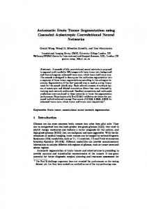
Figure 1: Generic flow chart of proposed method for brain tissue segmentation.
60
proposed segmentation method for this paper consists of several parts which are shown in Fig. 1. In the following, the details of different parts of the algorithm are discussed in details. 2.1. Image data and ground truth Data from MRBrainS13 were used, comprising twenty 3T MRI brain exami-
65
nations from twenty different patients. All subjects were above 50 years old with diabetes and matched control with varying degree of atrophy and white matter lesions. Each examination consists of 3 series of MRI images: T1-weighted, T1weighted inversion recovery and T2-FLAIR. All the series were aligned with each other using a deformable registration method. The voxel size of provided data
70
were 0.95mm×0.95mm×3.0mm. From the twenty available datasets, five cases were provided with manual segmentation (ground truth) for training purposes. The labels for the remaining 15 datasets were kept away from the participant for evaluating the performance of each proposed method. Manually segmented images consist of nine classes in total, including cortical Gray Matter (GM), basal 4
75
ganglia, White Matter (WM), White Matter Lesions (WML), Cerebro-Spinal Fluid in the extracerebral space (CSF), ventricles, cerebellum, brainstem and background. However, for the evaluation, only the three classes GM, WM and CSF were considered, in which Cortical GM and basal ganglia were both considered as GM, and WM and WML were both considered as WM [3]. Cerebellum
80
and brainstem were excluded when evaluating the segmentation accuracy. 2.2. Preprocessing The aim of preprocessing is to prepare the data in a suitable way to be fed to the classifier. In this work, the following preprocessing steps were applied to the data before sending them to the classifiers.
85
2.2.1. Bias field correction Intensity inhomogeneity is a common artifact in MRI images. We used N4ITK to remove the bias field [20]. It is worth noting that the MRBrainS13 datasets have been processed with another bias-field correction tool. Nevertheless, we found N4ITK could further improve the homogeneity, thus lead to
90
better segmentation results. 2.2.2. Histogram matching In this step, the histograms of all datasets were matched to that of the first dataset. This step is important for preventing the network from being confused by varying intensity range. Histogram matching was performed using
95
the HistogramMatchingImageFilter in Insight Segmentation and Registration Toolkit (ITK) [21]. 2.2.3. Skull stripping Since non-brain tissues, such as the skull, have a major impact on segmentation results, it is important to remove them to increase the accuracy of segmen-
100
tation. Skull stripping was performed using a shape model-based level set on T1-weighted inversion recovery images based on [22], [9]. After applying skull stripping, any voxels outside of the brain were mapped to zero as background. 5
2.2.4. Normalizing data To remove outlier intensity, the 4th and the 96th percentile of each dataset 105
were calculated as boundary values, and all voxels below and above these calculated values were clipped off and mapped to the derived boundary values. All images were normalized to have zero mean and a standard deviation of one. 2.3. Feature Extraction As the input to the network, features were extracted via two separate ap-
110
proaches. One set of features were conventional intensity-based and spatial-based features. From the images, the same features as in [11] were extracted, described as follows: • Intensities (I) of different channels (T1-weighted and T2-FLAIR)
115
• The intensity after convolution with a Gaussian kernel with σ = 1, 2, 3 mm2 • The gradient magnitude of the intensity (GMI) after convolution with a Gaussian kernel with σ = 1, 2, 3 mm2 • The Laplacian of the intensity (LI) after convolution with a Gaussian
120
kernel with σ = 1, 2, 3 mm2 • Normalized spatial coordinates (NSC) of each voxel (x, y, z), divided by the length, width, and height of the brain, respectively. The intensity of the T1-IR channel was not used as a direct feature, since it had large variability which degraded the segmentation results. In total, 32 features
125
were extracted and used in this stage of the method. Another important set of features, here used as extra channels, were the results from the shape model-based level set method, which are described in the next section.
6
2.4. Shape Context generation based on level set 130
In addition to the local appearance features that are encoded in the filtered local intensities, we also try to put the local points into a global shape context. This is done by first performing a rough segmentation of various brain structures and then using the signed distance maps from those structure surfaces as additional features. In this study, we extracted six interfaces, namely the inner
135
surface of the skull, the surface of the lateral ventricles and basal ganglia, the inner and outer surfaces of the cortical GM, and the mid-surface of the cortical gray matter. For the surface of the skull, lateral ventricles and basal ganglia, we used a threshold-based level set method guided by statistical shape priors. The segmentation was carried out in a hierarchical manner [23], i.e. the
140
skull is segmented first and its transform is used to initialize the position of the smaller structures, while its boundary limits the latter’s propagation. To segment the cortical gray matter, a surface skeleton-guided level set method reported in [9] was implemented. The principle of this method is to consider the cortical gray matter as a blanket that can be represented with a skeleton
145
surface s with slowly varying thickness r. The skeleton surface s is estimated by first finding the mid-surface of the WM-GM and GM-CSF interfaces that are extracted via the threshold-based level set method, and then refined with local intensity analysis at the top/bottom of the gyri/sulci. The thickness function r is set to 1.35 uniformly, i.e. assuming the thickness of cortical GM to be 2.7mm
150
everywhere. This parametric shape model is then used to regularize the propagation of the threshold-based level set function to refine the segmentation of the the WMGM and GM-CSF interfaces. By tuning the weighting factors of shape prior term and the image term, the distance between the interfaces and the skeleton
155
surface is allowed to vary smoothly between 0.35mm to 2.35mm, depending on the local intensity profile. The thresholds that separate WM-GM and GM-CSF are determined through histogram analysis. A more detailed description of this method can be found in [9]. Notice that, unlike other auto-context approaches where the feature represents the probability of one voxel belonging to a class, 7
Figure 2: Network Structure with three different layers. The input layer consists of 37 nodes representing the features. The hidden layer consist of 100 hidden nodes, and the output layer consists of 6 nodes representing each of the segmentation classes.
160
the shape context feature encodes each point’s distance to the surface of a brain structure. 2.5. Classifier Training An ANN based classifier is used as the backbone of the proposed algorithm. The Multilayer Perceptron approach was chosen, which provided relatively ac-
165
curate results and needed considerably shorter training time compared to other methods based on ANN. Fig. 2 shows the architecture of the proposed network.
Network training was performed by using a back propagation algorithm [24], [25]. This method uses each set of pattern in the training set to minimize the 170
error function using gradient descent. The error function for the pth pattern are defined by Ep =
1X (tpk − ypk )2 2
(1)
k
where tpk and ypk are the target and output vectors corresponding to the pth input pattern, respectively. The whole system error can be derived from E=
1 X Ep P p 8
(2)
175
where P is the total number of patterns in the training set. The learning rule in the back propagation algorithm for updating network weights is the generalized delta rule, which calculates the weight updates from output to input layer as follows:
wjk (t + 1) = wjk (t) − η
∂Ep (t) ∂wjk (t)
(3)
wij (t + 1) = wij (t) − η
∂Ep (t) ∂wij (t)
(4)
where wjk is the weight index which connects the hidden node j to the output 180
node k and wij connects the input node i to the hidden node j. In order to prevent the network to get stuck in local minima, a momentum term was used to moderate the weight update in each iteration, as described in [24]. For training set, n × 10000 voxels were randomly selected from n training
185
datasets within the brain region excluding the cerebellum and the brain stem. For each voxel, 37 features (32 image features plus 5 shape context features) and the corresponding labels were passed through the network. The training label includes 6 classes: WML, WM, Cortical GM, basal ganglia, ventricles and CSF. The ANN training was set to stop after 1000 iterations.
190
2.6. Image Segmentation and Post-processing For segmenting the test dataset, all voxels were passed through the trained classifier, which in turn output the probabilities of the voxel belonging to each of the 6 classes. The voxel was assigned to the class given the highest probability. Networks were trained with six labeled classes, and thus the network results
195
also included six classes. These six classes were merged to form the final three segmentation parts (i.e. WM, GM and CSF) following the rules described in [3].
9
2.7. Accuracy Analysis Segmentation results were compared to the ground truth based on the Dice 200
similarity index, the Absolute Volume Difference (AVD) similarity index, and 95th-percentile of the Hausdorff Distance (HD) index [3]. While the Dice coefficient indicates how the two masks overlap with each other, HD gives the largest distance between two contours. AVD, on the other hand, can indicate whether there is a systematic error with volume measurement. Background, cerebellum
205
and the brain stem were excluded from the validation phase.
3. Results All experiments were performed on a single desktop computer. For preprocessing and post-processing steps an Intel Xeon E5-2630 2.40 GHz CPU was utilized. The MLP algorithm was implemented in MATLAB (version 2016a) 210
and trained on GPU (NVIDIA GTX 1070, 8GB). The level set method was implemented in C++ and running on CPU. The training time was around 2 minutes for ANN inference and around 9 minutes for the shape model level set method. The running time of the trained ANN for segmenting a 3D volume was approximately 9 seconds, while the shape model level set method took 3-4
215
minutes to generate the shape context. The proposed MLP with shape context method (MLP-shape) was first tested on the 5 training datasets and compared with an MLP with plain features (MLPplain) and the shape model guided levelset method (LS-shape) that generated the shape context. For the shape context generation, the statistical shape mod-
220
els described in section 2.4 were generated using all 5 training datasets and applied to the 5 training datasets, while the ANN-based voxel classification was tested using the leave-one-out method. MLP-shape and MLP-plain share the same set of intensity and spatial features described in section 2.3. Table 1 compares the performances of these three methods on the 5 training datasets.
225
In almost all cases, MLP-shape delivers better segmentation results than using MLP with no shape context or using shape based levelset alone.
10
Table 1: Effect of using shape context features
Method
Dice(%)
Dice(%)
Dice(%)
Dice(%)
Dice(%)
ICV
Brain
CSF
WM
GM
MLP-plain
98.37
94.61
84.52
85.56
82.74
LS-shape
96.79
94.48
78.34
87.74
82.56
MLP-shape
98.39
95.17
85.48
87.50
84.71
Table 2: Effectiveness of selected features
Dropped set of features
Dice(%)
Dice(%)
Dice(%)
CSF
WM
GM
w/o Filtered I
84.55
84.23
82.11
w/o Filtered GMI
83.38
73.80
78.70
w/o Filtered LI
84.61
84.95
82.75
w/o NSC
84.33
85.49
82.37
In order to investigate the effectiveness of other selected features besides the shape context features, sets of experiments were performed by dropping one set of features at a time and training classifier with rest of the features. The average 230
results of these experiments using leave one out method are shown in Table 2 for CSF, WM and GM. Fig. 3 and Fig. 4 show the effect of skull stripping and data normalization. The final results after segmentation with the proposed algorithm are shown in Fig. 5. The first row shows three raw input slices. The second row shows the
235
segmentation results of 3 classes, and the third row shows the misclassified pixels in those slices. Table 3 summarizes the performance of the proposed method on the 15 testing datasets. In this case, the network was trained on all 5 training datasets. MLP-plain was not tested on the real testing cases, due to limited number
240
of submission allowed for each team. The evaluation was performed by MR11
50
50
100
100
150
150
200
200
50
100
150
200
50
100
150
200
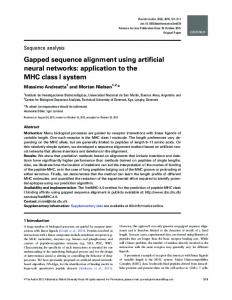
Figure 3: Non-brain tissue removal for a sample slice (25th) from first dataset on T1-weighted scan: Raw image on the left and skull-stripped image on the right
50
50
100
100
150
150
200
200
50
100
150
200
50
100
150
200
Figure 4: Removing extremely high and low values for a sample slice (25th) from first dataset on T1-weighted inversion recovery scan: On the left raw image and on the right the image after applying this preprocessing step. (T1-IR shows the effect of this preprocessing step clearly due to large variation of the intensity values this channel)
12
50 100 150 200
50 100 150 200 50 100 150 200
50 100 150 200
50 100 150 200 50 100 150 200
50 100 150 200 50 100 150 200
50 100 150 200
50 100 150 200 50 100 150 200
50 100 150 200 50 100 150 200
50 100 150 200
50 100 150 200 50 100 150 200
50 100 150 200
50 100 150 200
Figure 5: Examples of segmentation results for three slices (10, 25, 35) of the 5th dataset. The first row shows the raw T1-weighted scan, the second row shows the segmentation result, and the third row shows the misclassified pixels in these three sample slices. Cerebellum and brainstem were removed manually using the ground truth.
13
Table 3: Comparison of results of selected algorithms on the MRBrainS13 data
Team
GM
WM
CSF
DC(%)
HD(mm)
AVD(%)
DC(%)
HD(mm)
AVD(%)
DC(%)
HD(mm)
AVD(%)
CU/DL
86.15
1.47
6.42
89.39
1.94
5.84
83.96
2.28
7.44
CU/DL2
86.12
1.45
6.60
89.46
1.94
6.05
84.25
2.19
7.69
MDGRU
85.4
1.55
6.09
88.98
2.02
7.69
84.13
2.17
7.44
LS-Shape
82.56
2.83
7.63
87.74
2.46
7.15
78.34
3.09
15.63
MLP-shape
84.78
1.71
6.02
88.47
2.36
7.66
82.76
2.32
6.73
Brains13 challenge organizers, who also provided the extensive comparison to other segmentation approaches on the same datasets. The proposed method (labeled as STH on the challenge website) was ranked 7th taking into account all segmentation scores, and was ranked 4th for segmenting brain tissue ( GM 245
+ WM ). In total, 37 teams participated in the challenge at the time of writing this report. In Table 3 the first three rows show the results of top three teams in the challenge respectively. While the propose method in general has lower Dice score, the largest differences between the top ranked method and the proposed method is only 1.37%.
250
4. Discussion The main contribution of this study is proposing a new segmentation algorithm which incorporates the shape prior into the machine learning framework by combining an ANN-based learning algorithm and a shape model-based level 255
set method. This hybrid solution delivers better performance compared to either of them individually (cf. Tables 1). Through visual inspection, we found that adding the shape prior knowledge helped the algorithm to better recognize the basal ganglia areas inside the brain than the ANN algorithm using only 14
image features. When compared with the pure statistical shape guided level set 260
implementation, the improvement is more on the edges of the brain structures. It may be noted that the shape context need not be very precise for the ANN to learn useful information from these features. In our implementation, the modelbased level set method uses only the intensity of the T1 image to perform the segmentation, while ANN uses 32 image features of all 3 MRI sequences. Also
265
when compared to auto context models [4], [12] (rank 8th and 9th in the challenge), the shape context information seems to be better than multi-iteration auto-contexting and only needs a single iteration. It should be pointed out that although our implementation has only been tested on brain images, the proposed framework is rather general can be easily
270
extended to segment other anatomical structures with relatively small changes. In fact, the proposed volumetric shape context features can be easily integrated into many other machine learning based image segmentation methods, such as SVM, random forest or even the deep learning methods. In a recent study from our group [26], we have tested to integrate the shape context with the random
275
forest method and Haar-like features, and promising results were reported in combination with other improvements. It is also worth noticing that the shape context is not limited to the volumetric statistical shape models. Via a simple mesh voxelization, other types of shape priors such as active shape models (ASM) can also be used as shape context.
280
In comparison to the deep learning based methods [13], [14], [15],[16], the proposed method is mostly inferior in terms of segmentation accuracy. But the differences in Dice scores are relatively small, often below 1%. On the other hand, the proposed method produces smaller Absolute Volume Difference(AVD) to the ground truth, especially for CSF and brain volume measurement, on
285
which our method was ranked in the first and second place respectively. Another advantage of the proposed method over deep learning approaches is much shorter training time. The training time of the top 3 winning methods was 1 day, 1 day and 2 days respectively and their training was performed on much more powerful GPUs (NVIDIA GTX TITAN X). As both the proposed method and 15
290
the deep learning methods are learning-based methods, from our experience, the networks need to be retrained if the imaging protocol is changed or simply moved to another type of scanner. When considering both the training and testing processes, our approach could be more attractive to be deployed in clinical settings.
295
Beside the shape context features, the other 32 features have been suggested in previous studies by [11]. Table 2 shows the effectiveness of each set of selected features by excluding them from the training process. As the results suggest, dropping the NSC features has the least effect on segmentation results while dropping gradient magnitude features degrades results considerably. Since we
300
want to achieve the best possible scores, for the final submission, we included all the features, no matter how small the contribution is. During the study, we also explored different architectures of the ANN. For example changing the number of node and layers, however, no significant improvement was observed. A number of well-known classifiers were tested in
305
the frame of this work. SVM, MLP, learning vector quantization (LVQ) and radial basis function (RBF) were tested as the main classifier. Between these classifiers, SVM and MLP achieved slightly better performance when tried for training dataset. The training time of MLP (on GPU) was much shorter compared to SVM. Therefore, MLP was chosen as the final classifier for this study.
310
As seen in Fig. 5, most of the segmentation errors within the brain occurred at the border between different brain tissues, where the inter-observer variation of the manual delineation could also be high. However, a single ground truth segmentation was generated for each testing data through consensus sessions, so the inter-observer variation of the segmentation accuracy is not available.
315
Yet, when comparing the Dice coefficients of the top 3 methods for each brain structure, the variation is mostly below 1%. In our experiments, skull stripping was found to be a prominent source of error. To investigate how much it could affect the results, one test was executed with the proposed skull stripping algorithm and one test was executed by using
320
manual segmentation for skull striping (i.e. perfect mask). The results of this 16
approach suggest that approximately 2% of the error for segmenting ICV and 5% of the error for segmenting CSF was related to skull stripping. It had very a small effect on the GM segmentation and almost no effect on WM segmentation. Another challenge in processing the MRBrainS13 data is to handle the WML 325
class (MS lesion) properly. While running the leave-one-out test, we noticed for one of the datasets (patient 2), that the Dice index of WM was considerably lower compared to other datasets. After further investigation on this specific dataset, it was revealed that this 3D volume consisted of a greater fraction of WML compared to other datasets. This suggests that for the training, there
330
needs to be a sufficient number of random samples within the WML regions to ensure correct classification of this specific tissue type. There are a number of limitations with the current study. First, the number of training and test cases are relatively small, which makes it difficult to predict how well the method will perform given plenty of training data. Second, the
335
proposed segmentation pipeline does not contain an explicit model of the bias field that often occurs in clinical images. For inhomogeneity correction, it must rely on third-party software such as SPM, which was used by the challenge organizer to preprocess the images [3]. Thirdly, for creating the shape model of the cortex, the cortical thickness was universally set to 2.7mm, which is not
340
ideal for patients with brain atrophy; an adaptive approach through iterative cortical thickness estimation might give better results.
5. Conclusion In this paper, a fully automatic method has been proposed, which incorporates the shape prior into the machine learning framework by combining an 345
ANN-based learning algorithm and a shape model-based level set method. Results for segmenting WM, GM and CSF of the brain using the proposed method were relatively accurate with acceptable standard deviation while the training and testing time were considerably shorter compared to other methods. Further investigation is needed for developing the current method to improve the
17
350
accuracy. Moreover, the potential generalization of the proposed algorithm to other fields of medical imaging segmentation is open for further studies.
References [1] I. Despotovi´c, B. Goossens, W. Philips, Mri segmentation of the human brain: challenges, methods, and applications, Computational and mathe355
matical methods in medicine 2015. [2] M. A. Balafar, A. R. Ramli, M. I. Saripan, S. Mashohor, Review of Brain MRI Image Segmentation Methods, Artificial Intelligence Review 33 (3) (2010) 261–274. [3] A. Mendrik, K. Vincken, H. Kuijf, M. Breeuwer, W. Bouvy, J. de Bresser,
360
A. Alansary, M. de Bruijne, A. Carass, A. El-Baz, A. Jog, R. Katyal, A. Khan, F. van der Lijn, Q. Mahmood, R. Mukherjee, A. van Opbroek, S. Paneri, S. Pereira, M. Persson, M. Rajchl, D. Sarikaya, O. Smedby, C. Silva, H. Vrooman, S. Vyas, C. Wang, L. Zhao, G. Biessels, M. Viergever, MRBrainS Challenge: Online Evaluation Framework for Brain Image Seg-
365
mentation in 3T MRI Scans, Computat Intellig Neuroscience. [4] P. Moeskops, M. A. Viergever, M. J. N. L. Benders, I. Iˇsgum, Evaluation of an automatic brain segmentation method developed for neonates on adult MR brain images, in: SPIE Medical Imaging, International Society for Optics and Photonics, 2015, p. 941315.
370
[5] A. Mendrik, Mrbrains website. URL http://mrbrains13.isi.uu.nl [6] M. Rajchl, J. Baxter, A. J. McLeod, J. Yuan, W. Qiu, T. M. Peters, Asets: Map-based brain tissue segmentation using manifold learning and hierarchical max-flow regularization, in: Proceedings of the MICCAI Grand
375
Challenge on MR Brain Image Segmentation (MRBrainS’13), 2013.
18
[7] Q. Mahmood, M. Alipoor, A. Chodorowski, A. Mehnert, M. Persson, Multimodal mr brain segmentation using bayesianbased adaptive mean-shift (bams), in: Proceedings of the MICCAI WorkshopsThe MICCAI Grand Challenge on MR Brain Image Segmentation (MRBrainS13), 2013. 380
[8] R. Katyal, S. Paneri, M. Kuse, Gaussian intensity model with neighborhood cues for fluid-tissue categorization of multi-sequence mr brain images, in: Proceedings of the MICCAI WorkshopsThe MICCAI Grand Challenge on MR Brain Image Segmentation (MRBrainS13), 2013. ¨ Smedby, Fully automatic brain segmentation using model[9] C. Wang, O.
385
guided level sets and skeleton-based models, Proceedings of the MICCAI Grand Challenge on MR Brain Image Segmentation (MRBrainS’13). [10] D. Sarikaya, L. Zhao, J. J. Corso, Multi-atlas brain mri segmentation with multiway cut, in: Proceedings of the MICCAI WorkshopsThe MICCAI Grand Challenge on MR Brain Image Segmentation (MRBrainS13), 2013.
390
[11] A. van Opbroek, F. van der Lijn, M. de Bruijne, A. V. Opbroek, F. V. D. Lijn, M. D. Bruijne, Automated Brain-Tissue Segmentation by MultiFeature SVM Classification, Bigr.Nl. [12] L. Wang, Y. Gao, F. Shi, G. Li, J. H. Gilmore, W. Lin, D. Shen, LINKS: Learning-based multi-source IntegratioN frameworK for Segmentation of
395
infant brain images, NeuroImage 108 (2015) 160–172. [13] H. Chen, Q. Dou, L. Yu, J. Qin, P.-A. Heng, VoxResNet: Deep voxelwise residual networks for brain segmentation from 3D MR images, NeuroImage. ¨ C [14] O. ¸ i¸cek, A. Abdulkadir, S. S. Lienkamp, T. Brox, O. Ronneberger, 3D U-Net: learning dense volumetric segmentation from sparse annotation,
400
in: International Conference on Medical Image Computing and ComputerAssisted Intervention, Springer, 2016, pp. 424–432. [15] S. Andermatt, S. Pezold, P. Cattin, Multi-dimensional gated recurrent units for the segmentation of biomedical 3D-data, in: International Workshop on 19
Large-Scale Annotation of Biomedical Data and Expert Label Synthesis, 405
Springer, 2016, pp. 142–151. [16] M. F. Stollenga, W. Byeon, M. Liwicki, J. Schmidhuber, Parallel MultiDimensional LSTM, With Application to Fast Biomedical Volumetric Image Segmentation, in: Advances in Neural Information Processing Systems, 2015, pp. 2980–2988.
410
[17] A. M. Dale, B. Fischl, M. I. Sereno, Cortical surface-based analysis: I. segmentation and surface reconstruction, Neuroimage 9 (2) (1999) 179– 194. [18] J. Ashburner, K. J. Friston, Unified Segmentation, Neuroimage 26 (3) (2005) 839–851.
415
[19] F. Chen, H. Yu, R. Hu, X. Zeng, Deep learning shape priors for object segmentation, in: Proceedings of the IEEE Conference on Computer Vision and Pattern Recognition, 2013, pp. 1870–1877. [20] N. J. Tustison, B. B. Avants, P. A. Cook, Y. Zheng, A. Egan, P. A. Yushkevich, J. C. Gee, N4itk: improved n3 bias correction, IEEE transactions on
420
medical imaging 29 (6) (2010) 1310–1320. [21] L. G. Ny´ ul, J. K. Udupa, X. Zhang, New variants of a method of mri scale standardization, IEEE transactions on medical imaging 19 (2) (2000) 143–150. ¨ Smedby, Multi-organ Segmentation Using Shape Model [22] C. Wang, O.
425
Guided Local Phase Analysis, in:
Medical Image Computing and
Computer-Assisted Intervention{MICCAI} 2015, Springer International Publishing, pp. 149–156. URL
http://link.springer.com/chapter/10.1007/
978-3-319-24574-4{_}18
20
430
¨ Smedby, Automatic multi-organ segmentation in non[23] C. Wang, O. enhanced {CT} datasets using Hierarchical Shape Priors, Proceedings of the 22th International Conference on Pattern Recognition ({ICPR}). [24] S. Marsland, Machine Learning: an Algorithmic Perspective, CRC press, 2015.
435
[25] U. Bhattacharya, B. B. Chaudhuri, S. K. Parui, An MLP-based texture segmentation method without selecting a feature set, Image and vision computing 15 (12) (1997) 937–948. ¨ Smedby, Automatic heart and vessel segmentation [26] C. Wang, Q. Wang, O. using random forests and a local phase guided level set method, in: Interna-
440
tional Workshop on Reconstruction and Analysis of Moving Body Organs, Springer, Cham, 2016, pp. 159–164.
21