Automatic Classifier Fusion for Produce Recognition - DECOM-UFOP

Automatic Classifier Fusion for Produce Recognition Fabio Augusto Faria, Jefersson Alex dos Santos, Anderson Rocha and Ricardo da S. Torres RECOD Lab Institute of Computing University of Campinas Campinas, S˜ao Paulo, Brazil {ffaria,jsantos,rocha,rtorres}@ic.unicamp.br www.ic.unicamp.br/∼{ffaria,jsantos,rocha,rtorres}

Abstract—Recognizing different kinds of fruits and vegetables is a common task in supermarkets. This task, however, poses several challenges as it requires the identification of different species of a particular produce and also its variety. Usually, existing computer-based recognition approaches are not automatic and demand long-term and laborious prior training sessions. This paper presents a novel framework for classifier fusion aiming at supporting the automatic recognition of fruits and vegetables in a supermarket environment. The objective is to provide an effective mechanism for combining low-cost classifiers trained for specific classes of interest. The experiments performed demonstrate that the proposed framework yields better results than several related work found in the literature and represents a step forward automatic produce recognition in cashiers of supermarkets. Keywords-Produce Recognition; Ensemble of Classifiers; Diversity Measures;

I. I NTRODUCTION Fruit and vegetable recognition is a recurrent task in supermarkets [1], [2]. One common application is concerned with the definition of the price of a produce, given its identification. This is a challenging problem as it deals with both different species of fruits and vegetables (e.g., apple, orange, potatoes) and many varieties of a single produce species (for example, Golden Delicious, Akane, Gala, and Fuji are different varieties of apples) [2]. Usually, existing recognition approaches are not automatic and demand long-term and laborious previous training sessions. One attempt to address that problem concerns with the use of barcodes that are assigned to packages of fruits/vegetables. A drawback of this solution relies on the lack of freedom on choosing the produce of interest. Another solution consists in using booklets containing photos of fruits/vegetables that are browsed to properly determine their price. That solution, however, poses new challenges related to the memorization and the subjectivity in the recognition process. The automatic recognition of fruits and vegetables based on computer vision and image processing techniques represents a suitable alternative for the problem. In these methods, algorithms are used to encode visual properties (e.g., color, texture, and shape) of produce images into feature vectors,

and machine learning techniques are employed to classify those fruits/vegetables considering their features. Bolle et al. [1], for example, proposed the VeggieVision system, the first supermarket produce recognition system that used different visual properties (e.g., color, texture, density). The authors reported a recognition rate of 95%, but considered the top four responses of the recognition system. Rocha et al. [2], in turn, proposed the use of fusion techniques that consider classifiers associated with different image descriptors for automatic produce recognition. Their fusion approach consisted in dividing the recognition task into multiple two-class problems. Good recognition rates (∼ = 97%) are reported, but the solution uses a fixed number of classifiers. It combines outcomes of
N 2 = O(N ) SVM classifiers, where N is the number of 2 classes. Arivazhagan et. al. [3] also addressed the produce recognition problem by using a classifier based on a Minimum Distance Criterion. They used the same dataset released by [2], but the reported results are worse. The target application demands real-time and high recognition rate. Usually, however, existing works fail to address both requirements at the same time. Other challenges involving automatic produce recognition using computer vision methods rely on dealing with existing different appearance variations of fruits and vegetables, as well as pose and illumination changes during image acquisition. This paper aims at diminishing the impact of such problems by presenting a novel framework for non-linear fusion of classifiers aiming at supporting the automatic recognition of fruits and vegetables. The objective is to provide an effective mechanism for combining efficiently low-cost base classifiers trained for specific classes of interest. The novelty of the proposed work relies on the use of diversity measures to automatically assess the correlation of classifiers and then to determine the more appropriate ones to be combined. The proposed framework fits well the fruits and vegetables recognition task as it allows a continuous learning of suitable classifiers over time. The performed experiments demonstrate that the proposed framework yields better results than several related works found in the literature. The remainder of this paper is organized as follows. Section II presents related concepts necessary to understand

this paper. Section III describes the steps of the proposed framework for fusion of classifiers and for selecting the most appropriate classifiers based on diversity measures. Section IV shows the experimental protocol we devised to validate our work while Section V discusses the results. Finally, Section VI states our conclusions and future research directions. II. R ELATED C ONCEPTS The following subsections describe related concepts necessary to understand this paper. A. Adaboost (BOOST) The AdaBoost algorithm was proposed by Schapire [4]. It constructs a ensemble system (strong classifier) by repetitive evaluation of weak classifiers1 in a series of rounds (t = 1, . . . N ). In this section we breafly describe the binary AdaBoost proposed in [4]. The multiclass AdaBoost [5] is a variation of this strategy. Let A and B be the training and the validation sets (A∪B = T ), and let x be a sample (image). The strategy consists in keeping a set of weights Wt (x) over T , where t is the current round. These weights can be interpreted as a measure of the difficulty level to classify each training/validation sample. At the beginning, all the samples have the same weight, but in each round, the weights of the misclassified samples are increased. Thus, in the next rounds the weak classifiers are forced to classify the harder samples. For each round, the algorithm selects the best weak classifier ht (x) and computes a coefficient αt that indicates the degree of importance of ht (x) in the final strong classifier. It is given by: 1  1 + rt  (1) αt = ln 2 1 − rt P where rt = x cT (x)ht (x). In our implementation, the weak classifier is trained by using the training set A. The best weak classifier is selected based on the error on the validation set B. Therefore, the weights Wt+1 are computed for both A and B sets based on the current weights Wt : Wt (x) exp (−αt T (x)ht (x)) Wt+1 (x) ← X Wt (x) exp (−αt T (x)ht (x))

(2)

x

The classification error of classifier h is given by: X Err(h) = W (x)

(3)

x|h(x)B(x) H(cjm )}

Fig. 3.

Proposed framework for classifier fusion.

Fig. 4. The five steps for classifiers selection are: (a) Validation matrix MV ; (b) R lists sorted by diversity measures scores; (c) Rt lists with top t; (d) counts the number of occurrences of each classifier; (e) Selected classifiers |C ∗ |.

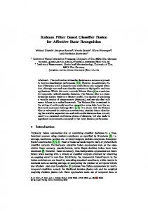
IV. E XPERIMENTAL P ROTOCOL This section presents the used image dataset, image descriptor, cross validation protocol, learning methods, diversity measures, and baselines. A. Supermarket Produce Dataset We have used freely available supermarket produce dataset2 proposed in [2]. That dataset comprises 2,633 images divided into 15 different categories: Plum (264), Agata Potato (201), Asterix Potato (182), Cashew (210), Onion (75), Orange (103), Taiti Lime (106), Kiwi (171), Fuji Apple (212), Granny-Smith Apple (155), Watermelon (192), Honeydew Melon (145), Nectarine (247), Williams Pear (159), and Diamond Peach (211). Figure 5 depicts some images of the dataset. B. Cross validation protocol In this paper, we consider a k-fold cross-validation protocol for all experiments we perform. In this protocol, the original dataset is randomly separated into k non-overlapping subsets. A subset is chosen for testing set, and the k−1 subsets are used for training a learning technique. The cross-validation process is repeated k times (rounds) and each subset is used only once as test set. The final result (the classification accuracy) from this process can be the arithmetic mean among all subsets. The main goal of this protocol is to test the entire dataset and reduce the variability among rounds (result of each round must be approximately equal). In our experiments, we have considered a 5-fold cross-validation protocol. Each training 2 http://www.ic.unicamp.br/∼rocha/pub/downloads/tropical-fruits-DB1024x768.tar.gz (As of May, 2012).

Fig. 5.

Supermarket Produce data set.

set (consisting of four rounds) can be further divided into validation and actual training (for instance, three folds can be used for training and the fourth for assessing the classifier being developed). In this sense, we use the 5-fold crossvalidation protocol again to further divide the training set into validation (one fold) and actual training (three folds). C. Image Descriptors Table I presents the color, texture, and shape descriptors we considered in our experiments. Given the produce recognition problem, the objective is to use the most complementary features as possible and rely on an effective combination

technique. Descriptor ACC [16] BIC [17] CCV [18] GCH [19] LAS [20] QCCH [21] EOAC [22]

Type Color Color Color Color Texture Texture Shape

TABLE I I MAGE DESCRIPTORS USED IN OUR EXPERIMENTS .

1) Color Autocorrelogram (ACC) [16]: The role of this descriptor is to map the spatial information of colors by pixel correlations at different distances. It computes the probability of finding in the image two pixels with color C at distance d from each other. For each distance d, m probabilities are computed, where m represents the number of colors in the quantized space. The implemented version quantized the color space into 64 bins and considered 4 distance values (1, 3, 5, and 7). 2) Border/Interior Pixel Classification (BIC) [17]: has been successful in many applications. The first step of the feature vector extraction process relies on the classification of image pixels into border or interior ones. When a pixel has the same spectral value in the quantized space as its four neighbors (the ones which are above, below, on the right, and on the left), it is classified as interior. Otherwise, the pixel is classified as border. Two histograms are computed after the classification: one for the interior pixels and another for the border ones. Both histograms are merged to compose the feature vector. The implemented version quantized the color space into 64 bins. 3) Color Coherence Vector (CCV) [18]: like GCH, it is recurrent in the literature. It uses an extraction algorithm that classifies the image pixels as “coherent” or “incoherent” pixels. This classification takes into consideration whether the pixel belongs or not to a region with similar colors, that is, coherent regions. Two color histograms are computed after quantization: one for coherent pixels and another for incoherent ones. Both histograms are merged to compose the feature vector. In our experiments, the color space was quantized into 64 bins. 4) Global Color Histogram (GCH) [19]: is one of the most commonly used descriptors, it uses an extraction algorithm which quantizes the color space in a uniform way and it scans the image computing the number of pixels belonging to each bin. The size of the feature vector depends on the quantization used. In the present work, the color space was split into 64 bins, thus, the feature vector has 64 values. 5) Local Activity Spectrum (LAS) [20]: this descriptor captures textures spatial activity in four different directions separately: horizontal, vertical, diagonal, and anti-diagonal. The four activity measures are computed for a pixel (i, j) by considering the values of neighboring in the four directions.

The values obtained are used to compute a histogram that is called local activity spectrum. Each component gi is quantized independently. In our experiments, each component was nonuniformly quantized into 4 bins, leading to a histogram with 256 bins. 6) Quantized Compound Change Histogram (QCCH) [21]: It uses the relation between pixels and their neighbors to encode texture information. This descriptor generates a representation invariant to rotation and translation. Its extraction algorithm scans the image with a square window. For each position in the image, the average gray value of the window is computed. Four variation rates are then computed by taking into consideration the average gray values in four directions: horizontal, vertical, diagonal, and anti-diagonal directions. The average of these four variations is calculated for each window position, they are grouped into 40 bins and a histogram of these values is computed. 7) Edge Orientation Autocorrelogram(EOAC) [22]: This is a shape descriptor. We chose this descriptor because it does not depend on segmentation to extract features. Its strategy is to classify the image edges according to two aspects: the edge orientation and the correlation between neighbor edges. The first step is to compute the image gradient from the input image. Then, the algorithm computes an edge orientation autocorrelogram. The feature vector is composed by the values from this auto-correlogram. In this implementation, we use angle quantization in 72 segments of 5◦ degrees each one; four distance values (1, 3, 5, and 7); the Sobel operator to compute the image gradient; and a gradient threshold equal to 25, as suggested in [22]. The final vector is comprised by 288 values. D. Learning Methods We have used seven learning methods in our framework: Na¨ıve Bayes (NB), Decision Tree (DT), Simple Logistic (SL), Na¨ıve Bayes Tree (NBT), k-Nearest Neighbors (kNN), using k = 1, k = 3, and k = 5. Such methods are simple and fast, being suitable to be combined in a real time recognition system. The idea of using different learning methods is that some descriptor might be better with specific methods. In this sense, a support vector machine was avoided here due to its known slow training time. Even though SVMs have sub linear time for testing, in a multi-class scenario it would need several binary SVMs to perform the multi-class classification as reported in [23]–[25]. The proposed framework aims at automatically finding suitable combinations of classifiers formed by descriptors and learning methods. We have used the implementation of those learning methods available in the WEKA3 data mining library. All learning techniques were used with default parameters. E. Diversity Measures Let M be a matrix containing the relationship between a pair of classifiers with percentage of concordance. Table II 3 http://www.cs.waikato.ac.nz/∼ml/weka

(As of May, 2012).

shows a relationship matrix M with percentage of hit and miss for two classifiers ci and cj . The value a is the percentage of images that both classifiers ci and cj classified correctly in the validation set. Values b and c are the percentage of images that cj hit and ci missed and vice-versa. The value d is the percentage of images that both classifiers missed. Hit cj Miss cj

Hit ci a c

Miss ci b d

using all patterns of class i as positive (+1) examples and the remaining class patterns as negative (-1) examples. We classify an input example x to the class with the highest response between the binary Adaboost classifiers. We also report the results of the methods described in [2] and [3], as they considered the same dataset in their experiments. In the case of [2], we consider two methods named Rocha BLDA and Rocha SVM-Fusion that use, respectively, Bagging of Linear Discriminant Analysis and SVM in the classification process.

TABLE II R ELATIONSHIP MATRIX M BETWEEN TWO CLASSIFIERS ci AND cj .

V. E XPERIMENTS

In [15], Kuncheva et al. present several measures to assess diversity, considering pairs of classifiers. Following their work, in our experiments, we have used Double-Fault Measure (DF M ), Q-Statistic (QST AT ), and Interrater Agreement k (IA). Those measures are defined as follows. DF Mi,j = d, QST ATi,j =

ad − bc , ad + bc

(6) (7)

This section discusses the results regarding the effectiveness and efficiency of the proposed framework. In the experiments, three different fusion approaches were conducted: SVM with RBF kernel considering h = 49 (FSVM-RBF-49) and h = 10 (FSVM-RBF-10) classifiers, and majority voting (MV-49). Note that the use of h = 49 refers to the use of all available base classifiers in the fusion process. We have used t = 10 in our experiments (see Line 11 of Algorithm 1) as we impose a constraint to classify each input as fast as possible for deployment of the system in a supermarket scenario similar to the one imposed in [2]. A. Effectiveness

IAi,j

2(ac − bd) = . (a + b)(c + d) + (a + c)(b + d)

(8)

The diversity is greater if the measures Double-Fault Measure, Q-Statistic and Interrater Agreement k are lower among pairs of classifiers ci and cj [15]. F. Baselines We have used seven different approaches as baselines: BAGG-3, BAGG-17, SVM-PK, SVM-RBF, BOOST, MVBOOST-7, and OVA-BOOST. We describe each baseline in the following. BAGG-3 and BAGG-17 rely on the bagging approach (Section II-B) using k = 3 and k = 7 iterations, respectively. Both are tested with BIC descriptor (Section IV-C). The configuration of the bagging-based methods are the same used in [2]. SVM-PK and SVM-RBF are classifiers based on support vector machines (Section II-C) using one image descriptor. SVM-PK uses polynomial kernels and SVM-RBF uses RBF kernels. The parameters used can be found [2]. BOOST and MV-BOOST-7 implement one multi-class adaboost (Section II-A) for each descriptor. The weak learner used is an SVM with polynomial kernel. In MV-BOOST-7, the descriptor results are combined by using the majority voting (MV) scheme. OVA-BOOST combines all descriptors using one binary Adaboost (Section II-A) for each dataset class. The binary Adaboost uses linear SVMs as weak learners. We used the One-vs-All (OVA) strategy to combine the binary classifiers. That strategy relies on training the ith classifier by

Table III presents the results organized in three parts: (1) Fusion Techniques; (2) Baselines form the literature which used the same dataset in their experiments; and (3) Baselines using just one image descriptor. All results consider the average classification accuracy considering a 5-fold crossvalidation protocol. As expected, FSVM-RBF-49 outperforms the baselines as it uses all configurations of classifiers and available descriptors. However, FSVM-RBF-10 performance is close to the one observed for FSVM-RBF-49, which means that the proposed selection framework based on diversity measures were able to select the most suitable classifiers (in this case, only 10 classifiers) to be combined without sacrificing much of the classification quality. Using less classifiers impacts the overall efficiency of the recognition system as discussed in the next section. FSVM-RBF-49 also yields better results than MV-49. One possible reason for that relies on its ability on producing a nonlinear combination of classifiers. For a better visualization, Figure 6 shows all results sorted by classification accuracy. B. Efficiency We conducted experiments on a 2.4GHz virtual machine with 1GB of RAM (running Linux) to assess the recognition time of the proposed framework. Our approach is composed by three steps: (1) extraction of feature vectors for all image descriptors; (2) classification using |C ∗ | classifiers; and (3) combination of |C ∗ | classifier outcomes with SVM. The complexity of Step 1 depends on the employed descriptors. In our case, that step takes ∼ = 0.5s. Step 2 takes less than 1s on average, since it uses low-cost

Supermarket Produce Dataset

100

Accuracy

95 90 85 80 75

Fig. 6.

Recognition Technique FSVM-RBF-49 FSVM-RBF-10 MV-49 MV-BOOST-7 OVA-BOOST Rocha BLDA [2] Rocha SVM-Fusion [2] Arivazhagan [3] BOOST-BIC SVM-PK-BIC BAGG-17-BIC BAGG-3-BIC SVM-RBF-ACC

1 0 0FSVM−RBF−49 1 FSVM−RBF−10 0 1 0MV−49 1

00 11 000 111 111 000 000 111 00 11 00 11 000 111 000 111 000 111 00 11 00 11 000 111 00 11 000 111 000 111 00 11 00 11 00 11 000 111 00 11 000 111 000 111 00 11 00 11 00 11 000 111 000 111 00 11 00 11 000 111 000 111 00011 111 00 11 00 00 11 000 111 000 111 00 11 000 111 00 11 000 111 000 111 00 11 00 11 00 11 000 111 000 111 00 11 000 111 000 111 000 111 00 11 00 00 00011 111 000 111 00 11 00 000 111 000 111 00011 111 00 11 0011 11 00011 111 0001

111 000 000 111 00 11 00 11 000 111 00 11 00 11 000 111 00 11 00 11 000 111 00 11 00 11 000 111 00 11 00 11 000 111 00 11 00 11 000 111 00 11 00 11 000 111 00 11 00 11 000 111 00 11 00 11 000 111 00 11 00 11 000 111 00 11 00 11 000 111 00 11 00 11 000 111 00 11 00 11 000 111 00 11 00 11 000 111 00 11 00 11 000 111 00 11 00 000 11 111

1 0 0 1 1 0 1 0 1 0 1 0 00 11 00 11 100110

Rocha BLDA Rocha SVM−Fusion BOOST−BIC SVM−PK−BIC MV−BOOST−7 BAGG−17−BIC BAGG−3−BIC Arivazhagan SVM−RBF−ACC OVA−BOOST

0110

Recognition−Techniques

Recognition techniques sorted by classification accuracy.

Accuracy 98.8% ± 0.9 98.0% ± 0.9 98.0% ± 1.1 93.4% ± 1.4 77.3% ± 0.8 97.0% ± 0.6 97.0% ± 0.4 ∼ = 86.0% 96.4% ± 1.0 96.1% ± 1.8 89.4% ± 1.8 87.3% ± 1.7 84.3% ± 2.7

TABLE III C LASSIFICATION EFFECTIVENESS OF THE PROPOSED FRAMEWORK AND BASELINES , WITH THEIR RESPECTIVE STANDARD DEVIATIONS .

measures, which allow the combination of non-correlated, highly-effective, and low-cost base classifiers. Our approach is suitable for real-time produce recognition due to two reasons: first, all used base classifiers are of low cost in terms of computational efforts; and second, only a reduced number of effective classifiers are combined. Future work includes the investigation of the use of other diversity measures and fusion techniques, as well as the development of an automatic way to find the final number of base classifiers to combine based on classification quality and time constraints imposed by the client. We have used part of the proposed framework for classifying remote sensing images and preliminary results are promising [26]. Therefore, we plan to continue investigating the use of the framework in other domains. ACKNOWLEDGEMENT

classifiers. Step 3 takes less than 0.1s, since it combines a few number of classifiers. Therefore, the average recognition time is less than 2s, for the FSVM-RBF-10, which considers h = |C ∗ | = 10 selected base classifiers. Note that Rocha et al. [2] reported that their method takes ∼ = 5s to recognize a new produce image, using a 2.1GHz machine with 2GB of RAM. VI. F INAL R EMARKS AND F UTURE W ORK This paper presented a new framework to combine classifiers aiming at supporting the deployment of produce recognition systems. The novelty of this work relies on the use of diversity measures to determine which base classifiers are suitable to be combined. The experiment results show that the proposed framework yields high classification accuracy rates in a reduced time. In fact, our framework is able to combine classifiers more effectively than baselines. Different from other approaches, our method is able to not only select classifiers, but also learn, indirectly, which descriptors (and therefore visual properties) are more appropriate for the target application. To keep the a high recognition rate with the minimum computational effort, our classifier selection strategy exploits the use of diversity

The authors are grateful to CAPES, CNPq, FAPESP (grants 2010/14910-0, 2010/05647-4, 2009/18438-7, 2009/18438-7, and 2008/58528-2), and Microsoft Research for the financial support. R EFERENCES [1] R. M. Bolle, J. H. Connell, N. Haas, R. Mohan, and G. Taubin, “Veggievision: A produce recognition system,” in IEEE WACV, Sarasota, USA, 1996, pp. 1–8. [2] A. Rocha, D. C. Hauagge, J. Wainer, and S. Goldenstein, “Automatic fruit and vegetable classification from images,” Elsevier COMPAG, vol. 70, no. 1, pp. 96 – 104, 2010. [Online]. Available: http: //www.sciencedirect.com/science/article/pii/S016816990900180X [3] S. Arivazhagan, R. N. Shebiah, S. S. Nidhyanandhan, and L. Ganesan, “Fruit recognition using color and texture features,” CIS Journal, 2010. [4] R. E. Schapire, “A brief introduction to boosting,” in Proceedings of the Sixteenth International Joint Conference on Artificial Intelligence, ser. IJCAI ’99, 1999, pp. 1401–1406. [5] Y. Freund and R. E. Schapire, “Experiments with a new boosting algorithm,” Update, pp. 148–156, 1996. [6] J. Friedman, T. Hastie, and R. Tibshirani, The Elements of Statistical Learning, 1st ed. Springer, 2001. [7] A. Rocha and S. Goldenstein, “Randomizac¸a˜ o progressiva para estegan´alise,” Master’s thesis, Campinas, SP, Brazil, 2006. [8] B. E. Boser, I. M. Guyon, and V. N. Vapnik, “A training algorithm for optimal margin classifiers,” in Proceedings of the fifth annual workshop on Computational learning theory, ser. COLT ’92, 1992, pp. 144–152.

[9] N. Cristianini and J. Shawe-Taylor, An Introduction to Support Vector Machines and Other Kernel-based Learning Methods. Cambridge University Press, 2000. [10] T. M. Cover, “Geometrical and statistical properties of systems of linear inequalities with applications in pattern recognition,” Electronic Computers, IEEE Transactions on, vol. EC-14, no. 3, pp. 326–334, 1965. [11] R. Herbrich, T. Graepel, and K. Obermayer, Large Margin Rank Boundaries for Ordinal Regression. Cambridge, MA: MIT Press, 2000, pp. 115–132. [Online]. Available: http://stat.cs.tu-berlin.de/publications/ papers/herobergrae99.ps.gz [12] T. Joachims, “Optimizing search engines using clickthrough data,” in International Conference on Knowledge Discovery and Data Mining, 2002, pp. 133–142. [13] Y. Cao, X. Jun, T. Liu, H. Li, Y. Huang, and H. Hon, “Adapting ranking svm to document retrieval,” in Proceedings of the 29th annual international ACM SIGIR conference on Research and development in information retrieval, 2006, pp. 186–193. [14] P. Hong, Q. Tian, and T. S. Huang, “Incorporate support vector machines to content-based image retrieval with relevant feedback,” in International Conference on Image Processing, 2000, pp. 750–753. [15] L. I. Kuncheva and C. J. Whitaker, “Measures of diversity in classifier ensembles and their relationship with the ensemble accuracy,” Machine Learning, vol. 51, pp. 181–207, May 2003. [16] J. Huang, R. Kumar, M. Mitra, W. Zhu, and R. Zabih, “Image indexing using color correlograms,” in IEEE CVPR, 1997, pp. 762–768. [17] R. Stehling, M. Nascimento, and A. Falcao, “A compact and efficient

[18] [19] [20] [21] [22]

[23] [24] [25] [26]

image retrieval approach based on border/interior pixel classification,” in ACM CIKM, 2002, pp. 102–109. G. Pass, R. Zabih, and J. Miller, “Comparing images using color coherence vectors,” in ACM Multimedia, 1996, pp. 65–73. M. Swain and D. Ballard, “Color indexing,” IJCV, vol. 7, no. 1, pp. 11–32, 1991. B. Tao and B. Dickinson, “Texture recognition and image retrieval using gradient indexing,” JVCIR, vol. 11, no. 3, pp. 327–342, 2000. C. Huang and Q. Liu, “An orientation independent texture descriptor for image retireval,” in ICCCS, 2007, pp. 772–776. F. Mahmoudi, J. Shanbehzadeh, A. Eftekhari-Moghadam, and H. Soltanian-Zadeh, “Image retrieval based on shape similarity by edge orientation autocorrelogram,” Elsevier Pattern Recog., vol. 36, no. 8, pp. 1725–1736, 2003. C. M. Bishop, Pattern Recognition and Machine Learning, 1st ed. Springer, 2006. A. Passerini, M. Pontil, and P. Frasconi, “New results on error correcting output codes of kernel machines,” IEEE TNN, vol. 15, no. 1, pp. 45–54, January 2004. A. Rocha and S. Goldenstein, “From binary to multi-class: divide to conquer,” in Visapp, Lisbon, Portugal, February 2009, pp. 323–330. F. A. Faria, J. A. Santos, R. da S. Torres, A. Rocha, and A. Falc˜ao, “Automatic fusion of region-based classifiers for coffee crop recognition,” in IEEE International Geoscience and Remote Sensing Symposium (IGARSS), Munique, Alemanha, July 2012.