A discussion of bilinear algorithms, tensor products, and the Chinese Remainder .... If both vectors are of the same size, M = N, the linear convolution is said to be of size N. ...... Maple V Programming Guide (Version A): Release 5. ... Prior to joining CHI Research, Anthony was a graduate student at Temple University where.
Automatic Derivation and Implementation of Fast Convolution Algorithms
A Thesis Submitted to the Faculty of Drexel University by Anthony F. Breitzman in partial fufillment of the requirements for the degree of Doctor of Philosophy January 2003
c Copyright 2003 ° Anthony F. Breitzman. All Rights Reserved.
ii
Dedications To Joanne, Anthony, and Taylor, for their patience and support.
iii
Acknowledgements First and foremost, I would like to thank my wife Joanne, who encouraged me throughout this process, and never complained about the endless nights and weekends spent on this project. I would like to thank my advisor, J. Johnson who not only guided me through this process, but provided insights and encouragement at critical moments. I also want to recognize other members of my committee for their thoughtful input: I. Selesnick, B. Char, H. Gollwitzer, and P. Nagvajara. During my studies I also worked full time. I want to thank CHI Research, Inc. for funding my studies, and my boss F. Narin for his flexibility throughout the process. Finally, I wish to thank my parents, Charles and Mary Lou Breitzman for giving me opportunities that they never had.
iv
Table of Contents List of Tables
. . . . . . . . . . . . . . . . . . . . . . . . . . . . . . . . . . . . . . . . . . . .
vii
List Of Figures . . . . . . . . . . . . . . . . . . . . . . . . . . . . . . . . . . . . . . . . . . . .
viii
Abstract
. . . . . . . . . . . . . . . . . . . . . . . . . . . . . . . . . . . . . . . . . . . . . . .
Chapter 1. Introduction
ix
. . . . . . . . . . . . . . . . . . . . . . . . . . . . . . . . . . . . . .
1
Summary . . . . . . . . . . . . . . . . . . . . . . . . . . . . . . . . . . . . . . . . . .
2
Chapter 2. Mathematical Preliminaries . . . . . . . . . . . . . . . . . . . . . . . . . . . . . .
5
1.1
2.1
Three Perspectives on Convolution . . . . . . . . . . . . . . . . . . . . . . . . . . . .
5
2.2
Polynomial Algebra
. . . . . . . . . . . . . . . . . . . . . . . . . . . . . . . . . . . .
6
2.2.1
Chinese Remainder Theorem . . . . . . . . . . . . . . . . . . . . . . . . . . .
7
2.2.2
Tensor Product . . . . . . . . . . . . . . . . . . . . . . . . . . . . . . . . . . .
9
Bilinear Algorithms . . . . . . . . . . . . . . . . . . . . . . . . . . . . . . . . . . . . .
10
2.3.1
Operations on Bilinear Algorithms . . . . . . . . . . . . . . . . . . . . . . . .
11
Linear Algorithms and Matrix Factorizations . . . . . . . . . . . . . . . . . . . . . .
13
2.3
2.4
Chapter 3. Survey of Convolution Algorithms and Techniques
. . . . . . . . . . . . . . . . .
15
Linear Convolution . . . . . . . . . . . . . . . . . . . . . . . . . . . . . . . . . . . . .
15
3.1.1
Standard Algorithm . . . . . . . . . . . . . . . . . . . . . . . . . . . . . . . .
15
3.1.2
Toom-Cook Algorithm . . . . . . . . . . . . . . . . . . . . . . . . . . . . . . .
15
3.1.3
Combining Linear Convolutions . . . . . . . . . . . . . . . . . . . . . . . . . .
17
3.2
Linear Convolution via Cyclic Convolution . . . . . . . . . . . . . . . . . . . . . . . .
18
3.3
Cyclic Convolution . . . . . . . . . . . . . . . . . . . . . . . . . . . . . . . . . . . . .
19
3.3.1
Convolution Theorem . . . . . . . . . . . . . . . . . . . . . . . . . . . . . . .
20
3.3.2
Winograd Convolution Algorithm . . . . . . . . . . . . . . . . . . . . . . . . .
22
3.3.3
CRT-Based Cyclic Convolution Algorithms for Prime Powers . . . . . . . . .
23
3.3.4
The Agarwal-Cooley and Split-Nesting Algorithms . . . . . . . . . . . . . . .
25
3.3.5
The Improved Split-Nesting Algorithm . . . . . . . . . . . . . . . . . . . . . .
26
3.1
Chapter 4. Implementation of Convolution Algorithms 4.1
. . . . . . . . . . . . . . . . . . . . .
29
Overview of SPL and the SPL Maple Package . . . . . . . . . . . . . . . . . . . . . .
29
4.1.1
29
SPL Language . . . . . . . . . . . . . . . . . . . . . . . . . . . . . . . . . . .
v 4.1.2 4.2
4.3
SPL Maple Package . . . . . . . . . . . . . . . . . . . . . . . . . . . . . . . .
31
Implementation Details of Core SPL Package . . . . . . . . . . . . . . . . . . . . . .
32
4.2.1
Core SPL Commands . . . . . . . . . . . . . . . . . . . . . . . . . . . . . . .
32
4.2.2
Core SPL Objects . . . . . . . . . . . . . . . . . . . . . . . . . . . . . . . . .
33
4.2.3
Creating Packages that use the SPL Core Package . . . . . . . . . . . . . . .
42
Implementation of Convolution Package . . . . . . . . . . . . . . . . . . . . . . . . .
42
4.3.1
The Linear Convolution Hash Table . . . . . . . . . . . . . . . . . . . . . . .
47
4.3.2
A Comprehensive Example . . . . . . . . . . . . . . . . . . . . . . . . . . . .
51
Chapter 5. Operation Counts for DFT and FFT-Based Convolutions
. . . . . . . . . . . . .
54
5.1
Properties of the DFT, FFT, and Convolution Theorem . . . . . . . . . . . . . . . .
54
5.2
DFT and FFT Operation Counts . . . . . . . . . . . . . . . . . . . . . . . . . . . . .
55
5.3
Flop Counts for Rader Algorithm . . . . . . . . . . . . . . . . . . . . . . . . . . . . .
55
5.4
Conjugate Even Vectors and Operation Counts . . . . . . . . . . . . . . . . . . . . .
56
5.5
Summary . . . . . . . . . . . . . . . . . . . . . . . . . . . . . . . . . . . . . . . . . .
58
Chapter 6. Operation Counts for CRT-Based Convolution Algorithms . . . . . . . . . . . . .
63
6.1
Assumptions and Methodology . . . . . . . . . . . . . . . . . . . . . . . . . . . . . .
63
6.2
Operation Counts for Size p (p prime) Linear Convolutions Embedded in Circular Convolutions . . . . . . . . . . . . . . . . . . . . . . . . . . . . . . . . . . . . . . . .
64
Operation Counts for Size mn Linear Convolutions Embedded in Circular Convolutions . . . . . . . . . . . . . . . . . . . . . . . . . . . . . . . . . . . . . . . .
65
6.4
Operation Counts for Any Size Cyclic Convolution . . . . . . . . . . . . . . . . . . .
68
6.5
Mixed Algorithms for Cyclic Convolutions . . . . . . . . . . . . . . . . . . . . . . . .
71
6.6
Summary . . . . . . . . . . . . . . . . . . . . . . . . . . . . . . . . . . . . . . . . . .
78
Chapter 7. Results of Timing Experiments . . . . . . . . . . . . . . . . . . . . . . . . . . . .
79
6.3
7.1
FFTW-Based Convolutions . . . . . . . . . . . . . . . . . . . . . . . . . . . . . . . .
79
7.2
Run-Time Comparisons . . . . . . . . . . . . . . . . . . . . . . . . . . . . . . . . . .
81
7.2.1
Cyclic Convolution of Real Vectors . . . . . . . . . . . . . . . . . . . . . . . .
81
7.2.2
Basic Optimizations for SPL Generated CRT Algorithms . . . . . . . . . . .
88
7.2.3
Is Improved Split-Nesting the Best Choice? . . . . . . . . . . . . . . . . . . .
90
7.2.4
Cyclic Convolution of Complex Vectors . . . . . . . . . . . . . . . . . . . . .
92
Mixed CRT and FFT-Based Convolutions . . . . . . . . . . . . . . . . . . . . . . . .
92
7.3
vi 7.3.1
Generalizing Mixed Algorithm Timing Results . . . . . . . . . . . . . . . . .
96
Chapter 8. Conclusions . . . . . . . . . . . . . . . . . . . . . . . . . . . . . . . . . . . . . . .
98
Bibliography . . . . . . . . . . . . . . . . . . . . . . . . . . . . . . . . . . . . . . . . . . . . . 100 Vita . . . . . . . . . . . . . . . . . . . . . . . . . . . . . . . . . . . . . . . . . . . . . . . . . . 102
vii
List of Tables
3.1
Operation Counts for Linear Convolution . . . . . . . . . . . . . . . . . . . . . . . . . .
28
4.1
Core Maple Parameterized Matrices
. . . . . . . . . . . . . . . . . . . . . . . . . . . .
34
4.2
Core Maple Operators
. . . . . . . . . . . . . . . . . . . . . . . . . . . . . . . . . . . .
36
4.3
Linear Objects Contained in the Convolution Package
. . . . . . . . . . . . . . . . . .
43
4.4
Bilinear SPL Objects Contained in the Convolution Package . . . . . . . . . . . . . . .
48
4.5
Utility Routines Contained in the Convolution Package . . . . . . . . . . . . . . . . . .
49
5.1
Flop Counts for various FFT’s and Cyclic Convolutions
. . . . . . . . . . . . . . . . .
59
5.2
Flop Counts for Linear Convolutions Derived from FCT and RFCT . . . . . . . . . . .
60
5.3
Flop Counts for FCT and RFCT Sizes 2-1024
61
6.1
Operation Counts for P-Point Linear Convolutions
. . . . . . . . . . . . . . . . . . . .
68
6.2
Different Methods for Computing 6-Point Linear Convolutions . . . . . . . . . . . . . .
69
6.3
Linear Convolutions that Minimize Operations for Real Inputs . . . . . . . . . . . . . .
73
6.4
Linear Convolutions that Minimize Operations for Complex Inputs
. . . . . . . . . . .
74
6.5
Comparison of Op Counts for Improved Split-Nesting versus FFT-Based Convolution . . . . . . . . . . . . . . . . . . . . . . . . . . . . . . . . . . . . . . . . . .
75
7.1
Run-Time for FFTW-Based Convolutions versus Mixed Convolutions of Size 3m
. . .
95
7.2
Run-Time for FFTW-Based Convolutions versus Mixed Convolutions of Size 5m
. . .
96
7.3
Run-Time for FFTW-Based Convolutions versus Mixed Convolutions of Size 15m . . .
96
. . . . . . . . . . . . . . . . . . . . . . .
viii
List of Figures
6.1
Percent of Sizes Where Improved Split-Nesting uses Fewer Operations than FFT-Based Convolution . . . . . . . . . . . . . . . . . . . . . . . . . . . . . . . . . . .
78
7.1
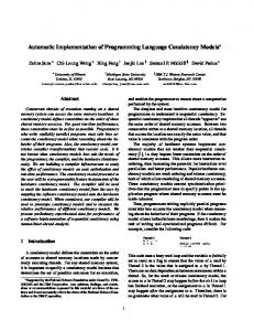
Run-Time Comparison of FFTW vs. Numerical Recipes FFT
. . . . . . . . . . . . . .
80
7.2
Example of an FFTW-Based Real Convolution Algorithm
. . . . . . . . . . . . . . . .
81
7.3
General FFTW-Based Real Convolution Algorithm . . . . . . . . . . . . . . . . . . . .
82
7.4
Example of an FFTW-Based Complex Convolution Algorithm . . . . . . . . . . . . . .
83
7.5
General FFTW-Based Complex Convolution Algorithm . . . . . . . . . . . . . . . . . .
84
7.6
Comparison of Convolution Algorithms on Real Inputs . . . . . . . . . . . . . . . . . .
85
7.7
Improved Split-Nesting (ISN) versus RFFTW Convolution for 3 Compilers . . . . . . .
86
7.8
Improved Split-Nesting (ISN) Operations Divided by Convolution Theorem Operations . . . . . . . . . . . . . . . . . . . . . . . . . . . . . . . . . . . . . . . . . . .
86
Average Run Time Per Line of Code for Various Size Convolution Algorithms . . . . .
87
7.9
7.10 Effect of Basic Optimizations on Run-Time for 3 CRT Convolutions
. . . . . . . . . .
90
7.11 Run-Time for Various Size 33 CRT-Based Convolutions and RFFTW . . . . . . . . . .
91
7.12 Comparison of Convolution Algorithms on Complex Inputs . . . . . . . . . . . . . . . .
92
7.13 Improved Split-Nesting (ISN) versus FFTW Convolution for 3 Compilers . . . . . . . .
93
7.14 Listing for Size 3m Mixed Algorithm
94
. . . . . . . . . . . . . . . . . . . . . . . . . . . .
ix
Abstract Automatic Derivation and Implementation of Fast Convolution Algorithms Anthony F. Breitzman Jeremy R. Johnson, Ph.D.
This thesis surveys algorithms for computing linear and cyclic convolution. Algorithms are presented in a uniform mathematical notation that allows automatic derivation, optimization, and implementation. Using the tensor product and Chinese Remainder Theorem (CRT), a space of algorithms is defined and the task of finding the best algorithm is turned into an optimization problem over this space of algorithms. This formulation led to the discovery of new algorithms with reduced operation count. Symbolic tools are presented for deriving and implementing algorithms, and performance analyses (using both operation count and run-time as metrics) are carried out. These analyses show the existence of a window where CRT-based algorithms outperform other methods of computing convolutions. Finally a new method that combines the Fast Fourier Transform with the CRT methods is derived. This latter method is shown to be faster for some very large size convolutions than either method used alone.
1
Chapter 1: Introduction Convolution is arguably one of the most important computations in signal processing, with more than 25 books and 5000 research papers related to it. Convolution also has applications outside of signal processing including the efficient computation of prime length Fourier Transforms, polynomial multiplication, and large integer multiplication. Efficient implementations of convolution algorithms are therefore always in demand. The careful study of convolution algorithms began with S. Winograd’s investigation of the complexity of convolution and related problems. Winograd in [29, 30] proved a lower bound on the number of multiplications required for convolution, and used the Chinese Remainder Theorem (CRT) to construct optimal algorithms that achieve the minimum number of multiplications. Unfortunately, to reach the theoretical minimum in multiplications often requires an inordinate number of additions that may defeat the gain in multiplications. These results spurred further study in the design and implementation of “fast” convolution algorithms. The research on this problem over the last 25 years is summarized in the books by Nussbuamer [19], Burrus and Parks [6], Blahut [4], and Tolimieri et al. [27]. In this thesis, the algorithms of Winograd and others that build upon Winograd will be referred to as CRT-based convolution algorithms. Much of past research has focused on techniques for reducing the number of additions by using near-optimal rather than optimal multiplication counts. Other authors, beginning with Agarwal and Cooley [1], have focused on using Winograd’s techniques to implement small convolution algorithms for specific sizes. These small algorithms are then combined to compute larger convolutions using various “prime factor” algorithms. This approach has had the greatest success in the application to computing prime size discrete Fourier transforms (DFT) via Rader’s theorem [21] and prime factor fast Fourier transforms (FFT) (see for example [5, 25]). Despite all of the development however, many questions remain about these algorithms. The main unanswered question is to determine the practicality of CRT-based algorithms over the full range of input sizes. In particular, a direct comparison of CRT algorithms versus FFT-based algorithms using the convolution theorem is needed. (See [27] for discussion of the convolution theorem). More generally, an exploration is needed to determine the best way to combine the various algorithms and techniques to obtain fast implementations and to ultimately optimize performance. One reason this has not been done is the difficulty in implementing CRT algorithms for general sizes, and the need to produce production quality implementations in order to obtain meaningful comparisons.
2 Another reason is that the various convolution algorithms and techniques lead to a combinatorial search problem for identifying optimal algorithms. The main goal of this thesis is to carry out a systematic investigation of convolution algorithms in order to obtain an optimal implementation and to determine the instances where CRT algorithms are better than FFT-based algorithms. In order to carry out this research, an infrastructure was developed for automatically deriving and implementing convolution algorithms. Previous work has been done in this direction, but most of these efforts have produced un-optimized straight-line code [1, 8]. More recent work by Selesnick and Burrus [22], has automated the generation of convolution algorithms without using straight-line code. Their work highlighted the structure in prime-power algorithms and showed how to utilize this structure to generate structured code. However the code produced was for MATLAB and does not produce an optimized implementation. Moreover, they do not provide tools to experiment with algorithmic choices nor arbitrary sizes. These limitations do not allow previous work to be used to systematically answer the performance question addressed here. This thesis discusses a research project that builds mainly on the work of Agarwal and Cooley [1] and Selesnick and Burrus [22], and aims to address the above issues and others. In short, the previous work is extended to examine convolution algorithms for any size N , building on the structure noted by Selesnick and Burrus [22], to automatically generate efficient structured computer code for CRT-based algorithms. Next, a performance study is undertaken to determine the viability of different approaches, and to ultimately compare CRT-based convolution algorithms with FFTbased techniques. This is the first such performance study based on run-time undertaken. These efforts build on earlier techniques for automating the implementation of FFT algorithms developed by Johnson et al. [13, 2] and are part of the SPIRAL project [24] whose aim is to automate the design, optimization, and implementation of signal processing algorithms.
1.1
Summary
The research has six components, corresponding to the six remaining chapters of the thesis. Each of the chapters is summarized here. • Chapter 2 discusses the mathematical preliminaries that will be needed in the remaining chapters. A discussion of bilinear algorithms, tensor products, and the Chinese Remainder Theorem is provided because in subsequent chapters it is shown that the various techniques developed over the years can all be shown to be generated via tensor products and the Chinese Remainder Theorem.
3 • Chapter 3 presents a uniform representation of various convolution algorithms discussed in the literature. This allows for easy comparison, analysis, and implementation of the algorithms, and also allows for the creation of an “algebra of algorithms,” which can be manipulated, combined, generated in a structured and automated way. This is not merely a matter of notation or style, but is a crucial foundation for systematically studying convolutions in the subsequent chapters. Ultimately this led to the discovery/development of a new algorithm “the improved split-nesting algorithm” that uses fewer operations than previously published algorithms. • Chapter 4 presents an infrastructure for experimenting, manipulating, and automatically generating convolution algorithms. This contribution is absolutely crucial to the success of this research for several reasons. First, these algorithms are error prone and difficult to program efficiently by hand except for very small cases. Second, a flexible framework and scripting language were necessary for determining how the various algorithms interact with one another, and for experimenting and assisting in the generation of the algorithms and operation counts used in the rest of the thesis. Last, the sheer magnitude of the testing procedure greatly exceeded any previous work, and would have been simply impossible to do by hand. For example, a size 77 cyclic convolution contains more than 50,000 lines of C code, while the entire tested set of sizes between 2 and 80 contains more than 319,000 lines of straight-line code and more than 196,000 lines of looped code. The timing process discussed in chapter 7 involved generating and compiling more than 10 million lines of C code. Doing such a project without an infrastructure would be simply impossible. • Chapter 5 builds upon the work of [9, 21, 23] to create baseline operation counts for all size Fast Fourier Transforms, which are then used to create baseline operation counts for convolutions created with the convolution theorem. These are then used in Chapter 6 to determine whether the CRT-based convolutions can be competitive (in terms of operation count) with FFT-based convolutions. • Chapter 6 undertakes an extensive analysis of operation counts for all linear and cyclic convolutions of size 1 to 1024, and identifies a window where these algorithms use fewer operations then FFT-based algorithms. Since there are multiple ways of computing linear convolutions of any given size, this involved an exhaustive search of more than 1.6 million algorithms. This is significant because for the 25 years that researchers have been studying these algorithms, no one has carefully analyzed under what conditions the algorithms would be competitive with
4 FFT-based algorithms. While operation count is not the best predictor of actual performance, it is a useful first step in analyzing performance. Moreover, operation count is unambiguous and allows definitive statements to be made. The key result is that the CRT-based algorithms use fewer operations than FFT-based algorithms for 90% of sizes between 2 and 200 for real input vectors, and in 48% of sizes between 2 and 100 for complex input vectors. This relatively small window can be exploited so that large (sizes up to 10,000 and beyond) convolution algorithms can be created that combine an FFT with a CRT-based convolution algorithm. These mixed algorithms in many cases use fewer operations than pure FFT-based or pure CRT-based convolutions. • Chapter 7 presents a performance analysis comparing the CRT-based algorithms with the best currently available FFT implementation. A window was found where these algorithms are faster than FFT-based algorithms in run-time. The mixed algorithm is shown to exploit these modest windows to create large fast algorithms that have faster run-times than pure FFT-based and pure CRT-based convolutions. The goal of this work was to determine whether CRT-based algorithms are practical, given current architectures where multiplications and additions have roughly the same cost. This thesis shows that not only are the algorithms viable as stand-alone algorithms, (based on both operation counts and run-times), but they also have a place in improving FFT-based convolution algorithms.
5
Chapter 2: Mathematical Preliminaries This chapter reviews the mathematical tools that we use in deriving convolution algorithms.
2.1
Three Perspectives on Convolution
Convolution can be viewed from three different perspectives: as a sum, a polynomial product, and a matrix operation. This allows polynomial algebra to be used to derive algorithms and the corresponding matrix algebra for manipulating and implementing algorithms. The linear convolution of the vectors u = (u0 , . . . , uM −1 ) and v = (v0 , . . . , vN −1 ) is a vector of size M + N − 1. If both vectors are of the same size, M = N , the linear convolution is said to be of size N . Definition 1 (Linear Convolution) Let u = (u0 , . . . , uM −1 ) and v = (v0 , . . . , vN −1 ). The i-th component of u ∗ v is equal to (u ∗ v)i =
N −1 X
ui−k vk , 0 ≤ i < 2N
(2.1)
k=0
If the vectors u = (u0 , . . . , uM −1 ) and v = (v0 , . . . , vN −1 ) are mapped to the polynomials u(x) =
M −1 X
ui xi and v(x) =
i=0
N −1 X
vj xj ,
j=0
then u ∗ v is mapped to the polynomial u(x)v(x). The linear convolution sum is also equivalent to the following matrix vector multiplication.
u0 u1 .. .
u ∗ v = uM −1
u0 u1 .. .
..
.
..
.
..
.
uM −1
u0 u1 .. .
v
(2.2)
uM −1 Cyclic convolution of two vectors of size N is obtained from linear convolution by reducing the indices i − k and k in Equation 2.1 modulo N .
6 Definition 2 (Cyclic Convolution) Let u = (u0 , . . . , uN −1 ) and v = (v0 , . . . , vN −1 ). The i-th component of the cyclic convolution of u and v, denoted by u ~ v, is equal to (u ~ v)i =
N −1 X
u(i−k)modN vk , 0 ≤ i < N
(2.3)
k=0
Circular convolution is obtained by multiplying the polynomials corresponding to u and v and taking the remainder modulo xN − 1. It can also be recast in terms of matrix algebra, as the product of a circulant matrix CircN (u), times the vector v,
u0
u1 .. u~v = . uN −2 uN −1
uN −1
uN −2
...
u1
u0 .. .
uN −1 .. .
... .. .
u2 .. .
...
u1
u0
uN −1
uN −2
...
u1
u0
v.
This matrix is called a circulant matrix because the columns of the matrix are all obtained by cyclically rotating the first column. A circulant matrix is generated by the shift matrix
SN
=
0
...
0
0
1
0
...
0
0 .. .
1 ..
.
0 ..
.
... .. .
0
...
0
1
1
0 0 , .. . 0
(2.4)
which is so named because when it is applied to a vector it cyclically shifts the elements. It is easy to verify that CircN (u) =
N −1 X
i ui SN .
(2.5)
i=0
2.2
Polynomial Algebra Elementary properties of polynomial algebras, in particular the Chinese remainder theorem
(CRT), can be used to derive convolution algorithms, and the regular representation can be used to convert from the polynomial view of convolution to the matrix view. Let f (x) be a polynomial with coefficients in a field F, and let F[x]/f (x) denote the quotient algebra of polynomials modulo f (x). Typically F will be the complex, C, or real, R, numbers depending on the convolution inputs;
7 however when deriving algorithms using the CRT, the rationals, Q or an extension of the rationals will be used depending on the required factorization of f (x). Linear convolution corresponds to multiplication in the polynomial algebra F[x], and cyclic convolution corresponds to multiplication in F[x]/xN − 1. The regular representation, ρ, of the algebra F[x]/f (x) is the mapping from F[x]/f (x) into the algebra of linear transformations of F[x]/f (x) defined by ρ(A(x))B(x) = A(x)B(x)
(mod f (x)),
where A(x) and B(x) are elements of F[x]/f (x). Once a basis for F[x]/f (x) is selected, the regular representation associates matrices with polynomials. Assume that deg(f (x)) = N . The dimension of F[x]/f (x) is N , and {1, x, x2 , . . . , xN −1 } is a basis for F[x]/f (x). With respect to this basis, ρ(x) = Cf , the companion matrix of f (x), and the regular representation of F[x]/f (x) is the matrix algebra generated by Cf . In particular, when f (x) = xN − 1, ρ(x) is SN and the regular representation of C[x]/(xn − 1) is the algebra of circulant matrices.
2.2.1
Chinese Remainder Theorem
The polynomial version of the Chinese Remainder provides a decomposition of a polynomial algebra, F[x]/f (x) into a direct product of polynomial algebras. Theorem 1 (Chinese Remainder Theorem) Assume that f (x) = f1 (x) · · · ft (x) in F where gcd(fi (x), fj (x)) = 1 for i 6= j. Then F[x]/f (x) ∼ = F[x]/f1 (x) × · · · × F[x]/ft (x) Where the isomorphism is given constructively by a system of orthogonal idempotents e1 (x), . . . , et (x) where ei (x)ej (x) ≡ 0 (mod f (x)) when i 6= j, ei (x)ei (x) ≡ 1 (mod f (x)), and e1 (x)+· · ·+et (x) ≡ 1 (mod f (x)). If A(x) = A1 (x)e1 (x) + · · · At (x)et (x), then A(x) ≡ Ai (x) (mod fi (x)). A more general version of this theorem with a proof can be found in [16]. Theorem 2 (Matrix Version of the CRT) Let R be the linear transformation, from the CRT, that maps F[x]/f (x) onto F[x]/f1 (x) × · · · × F[x]/ft (x): R(A(x)) = (A(x) mod f1 (x), . . . , A(x) mod ft (x)). Then Rρ(A) = (ρ(A1 ) ⊕ · · · ⊕ ρ(At ))R.
8 Proof Rρ(A)B
= R(AB) = (A1 B1 , . . . , At Bt ) = (ρ(A1 ) ⊕ · · · ⊕ ρ(At ))(B1 , . . . , Bt ) = (ρ(A1 ) ⊕ · · · ⊕ ρ(At ))RB
Since B is arbitrary the equation in the theorem is true. Example 1 Let f (x) = x4 − 1, and let f1 (x) = x − 1, f2 (x) = x + 1, and f3 (x) = x2 + 1 be the irreducible rational factors of f (x). Let A(x) = a0 + a1 x + a2 x2 + a3 x3 be an element of Q[x]/f (x) (coefficients could come from any extension of Q). Since A(x) mod f1 (x) = a0 + a1 + a2 + a3 , A(x) mod f2 (x) = a0 − a1 + a2 − a3 , and A(x) mod f3 (x) = (a0 − a2 ) + (a1 − a3 )x, 1 1 1 −1 R= 1 0 0 1
1 1 −1 0
1 −1 , 0 −1
with R(a0 , a1 , a2 , a3 )T = (A mod f1 , A mod f2 , A mod f3 ). It is easy to verify that e1 (x) = (1 + x + x2 + x3 )/4, e2 (x) = (1 − x + x2 − x3 )/4, and e3 (x) = (1 − x2 )/2 are a system of orthogonal idempotents. Therefore,
R−1
1/4 1/4 = 1/4 1/4
1/4 −1/4 1/4 −1/4
1/2 0 −1/2 0
0 1/2 . 0 −1/2
Consequently,
a0 a1 R a2 a3
a0 + a1 + a2 + a3 0 = 0 0
a3 a0 a1 a2
a2 a3 a0 a1
a1 a2 R−1 a3 a0
0 a0 − a1 + a2 − a3 0 0
0 0 a0 − a2 a1 − a3
0 0 . a3 − a1 a0 − a2
9
2.2.2
Tensor Product
The tensor product provides another important tool for deriving convolution algorithms. For this paper it is sufficient to consider the tensor product of finite dimensional algebras. Let U and V be vector spaces. A bilinear mapping β is a map from U × V −→ W such that β(α1 u1 + α2 u2 , v) =
α1 β(u1 , v) + α2 β(u2 , v)
β(u, α1 v1 + α2 v2 ) =
α1 β(u, v1 ) + α2 β(u, v2 )
It is easy to verify that convolution is a bilinear mapping. More generally, multiplication in any algebra is a bilinear mapping due to the distributive property. A vector space T along with a bilinear map θ : U × V −→ U ⊗ V is called a tensor product if it satisfies the properties: 1. θ(U × V ) spans T . 2. Given another vector space W and a bilinear mapping ϕ : U × V −→ W there exists a linear map λ : T −→ W with ϕ = θ ◦ λ. The tensor product, denoted by U ⊗ V , exists and is unique (see [16]). If U and V are finite dimensional and {u1 , . . . , um } and {v1 , . . . , vn } are bases for U and V , then {u1 ⊗ v1 , . . . , u1 ⊗ vn , . . . , um ⊗ v1 , . . . , um ⊗ vn } is a basis for U ⊗ V . It follows that the dimension of U ⊗ V is mn. Let A and B be algebras and let A ⊗ B be the tensor product of A and B as vector spaces. Let A1 , A2 ∈ A1 and B1 , B2 ∈ A2 , then A ⊗ B becomes an algebra with multiplication defined by (A1 ⊗ B1 )(A2 ⊗ B2 ) = A1 B2 ⊗ B1 B2 . It is clear from this definition, that the regular representation ρ(A ⊗ B) is equal to ρ(A) ⊗ ρ(B). When A1 and A2 are matrix algebras the tensor product coincides with the Kronecker product of matrices. Definition 3 (Kronecker Product) Let A be an m1 × n1 and B be an m2 × n2 matrix. The Kronecker product of A and B, A ⊗ B is the m1 m2 × n1 n2 block matrix whose (i, j) block, for 0 ≤ i < m1 and 0 ≤ j < n1 is equal to ai,j B. The following provides an example that will be used in the derivation of convolution algorithms. Example 2 F[x, y]/(f (x), g(y)) ∼ = F[x]/f (x) ⊗ F[y]/g(y)
10 Consider the bilinear map F[x]/f (x) × F[y]/g(y)
−→
F[x, y]/(f (x), g(y)) defined by
This map is onto since the collection of binomials xi y j span
(A(x), B(y)) −→ A(x)B(y).
F[x, y]/(f (x), g(y)). Property of the tensor product follows by setting λ(xi y j ) = ϕ(xi , y j ) for any other bilinear map ϕ. If deg(f ) = m and deg(g) = n, then {1, x, . . . , xm−1 } is a basis for F[x]/f (x) and {1, y, . . . , y n−1 } is a basis for F[y]/g(y). With respect to these bases, ρ(x) = Cf and ρ(y) = Cg . Using the basis {xi y j = xi ⊗ y j | 0 ≤ i < m, 0 ≤ j < n} ρ(x ⊗ y) = ρ(x) ⊗ ρ(y) = Cf ⊗ Cg . In particular, F[x]/(xm − 1) ⊗ F[y]/(y n − 1) corresponds to two-dimensional convolution and the regular representation has a block circulant structure. For example, when m = n = 2, the regular representation is given by
a0 a1 a0 (I2 ⊗ I2 ) + a1 (I2 ⊗ S2 ) + a2 (S2 ⊗ I2 ) + a3 (S2 ⊗ S2 ) = a2 a3
2.3
a1 a0 a3 a2
a2 a3 a0 a1
a3 a2 . a1 a0
Bilinear Algorithms
A bilinear algorithm [30] is a canonical way to describe algorithms for computing bilinear mappings. The purpose of this section is to provide a formalism for the constructions in [30] that can be used in the computer manipulation of convolution algorithms. Similar notation has been used by other authors [14, 27]. Definition 4 (Bilinear Algorithm) A bilinear algorithm is a bilinear mapping denoted by the triple (C, A, B) of matrices, where the column dimension of C is equal to the row dimensions of A and B. When applied to a pair of vectors u and v the bilinear algorithm (C, A, B) computes C (Au • Bv), where • represents component-wise multiplication of vectors.
Example 3 Consider a two-point linear convolution ·
¸ · ¸ u0 v0 u0 v0 ∗ = u0 v1 + u1 v0 . u1 v1 u1 v1
This can be computed with three instead of four multiplications using the following algorithm.
11 1. t0 ← u0 v0 ; 2. t1 ← u1 v1 ; 3. t2 ← (u0 + u1 )(v0 + v1 ) − t0 − t1 ; The desired convolution is given by the vectors whose components are t0 , t1 , and t2 . This algorithm is equivalent to the bilinear algorithm
1 0 tc2 = −1 1 0 0
2.3.1
0 1 −1 , 1 1 0
0 1 0 1 , 1 1 . 1 0 1
(2.6)
Operations on Bilinear Algorithms
Let B1 = (C1 , A1 , B1 ) and B2 = (C2 , A2 , B2 ) be two bilinear algorithms. The following operations are defined for bilinear algorithms. 1. [direct sum] B1 ⊕ B2 = (C1 ⊕ C2 , A1 ⊕ A2 , B1 ⊕ B2 ). 2. [tensor product] B1 ⊗ B2 = (C1 ⊗ C2 , A1 ⊗ A2 , B1 ⊗ B2 ). 3. [product] Assuming compatible row and column dimensions, B1 B2 = (C2 C1 , A1 A2 , B1 B2 ). As a special case of the product of two bilinear algorithms, let P and Q be matrices and assume compatible row and column dimensions. P B1 Q = (P C1 , A1 Q, B1 Q). These operations provide algorithms to compute the corresponding bilinear maps. Lemma 1 (Tensor product of bilinear mappings) Let B1 = (C1 , A1 , B1 ) and B2 = (C2 , A2 , B2 ) be two bilinear algorithms that compute β1 : U1 × V1 −→ W1 and β2 : U2 × V2 −→ W2 respectively. Then B1 ⊗ B2 computes the bilinear mapping β1 ⊗ β2 : U1 ⊗ U2 × V1 ⊗ V2 −→ W1 ⊗ W2 defined by β1 ⊗ β2 (u1 ⊗ v1 , u2 ⊗ v2 ) = β1 (u1 , v1 ) ⊗ β2 (u2 , v2 ). Proof B1 ⊗ B2 (u1 ⊗ u2 , v1 ⊗ v2 ) =
(C1 ⊗ C2 )((A1 ⊗ A2 )(u1 ⊗ u2 ) • (B1 ⊗ B2 )(v1 ⊗ v2 ))
= (C1 ⊗ C2 )(A1 u1 ⊗ A2 u2 ) • (B1 v1 ⊗ B2 v2 ) = (C1 ⊗ C2 )((A1 u1 • B1 v1 ) ⊗ (A2 u2 • B2 v2 )) = (C1 (A1 u1 • B1 v1 ) ⊗ (C2 (A2 u2 • B2 v2 )) = (C1 , A1 , B1 )(u1 , v1 ) ⊗ (C2 , A2 , B2 )(u2 , v2 ) = (β1 ⊗ β2 )(u1 ⊗ u2 , v1 ⊗ v2 ). The matrix version of the CRT can be used to construct a bilinear algorithm to multiply elements of F[x]/f (x) from a direct sum of bilinear algorithms to multiply elements of F[x]/fi (x).
12 Theorem 3 (Bilinear Algorithm Corresponding to the CRT) Assume that f (x) = f1 (x) · · · ft (x) in F[x], where gcd(fi (x), fj (x)) = 1 for i 6= j, and let (Ci , Ai , Bi ) be a bilinear algorithm to multiply elements of F[x]/fi (x). Then there exists an invertible matrix R such that the bilinear algorithm à R
−1
! t M (Ci , Ai , Bi ) R i=1
computes multiplication in F[x]/f (x).
In filtering applications it is often the case that one of the inputs to be cyclically convolved is fixed. Fixing one input in a bilinear algorithm leads to a linear algorithm. When this is the case, one part of the bilinear algorithm can be precomputed and the precomputation does not count towards the cost of the algorithm. Let (C, A, B) be a bilinear algorithm for cyclic convolution and assume that the first input is fixed. Then the computation (C, A, B)(u, v) is equal to (C diag(Au)B)v, where diag(Au) is the diagonal matrix whose diagonal elements are equal to the vector Au. In most cases the C portion of the bilinear algorithm is much more costly than the A or B portions of the algorithm, so it would be desirable if this part could be precomputed. Given a bilinear algorithm for a cyclic convolution, the matrix exchange property allows the C and A matrices to be exchanged.
Theorem 4 (Matrix Exchange) Let JN be the anti-identity matrix of size n defined by JN : i 7→ n − 1 − i for i = 0, . . . , N − 1, and let (C, A, B) be a bilinear algorithm for cyclic convolution of size N . Then (JN B t , A, C t JN ), where ()t denotes matrix transposition, is a bilinear algorithm for cyclic convolution of size N .
Proof −1 t Since JN SN JN = SN and JN = JN , CircN (u) = JN CircN (u)t JN . Therefore,
u~v
= CircN (u)v = (JN CircN (u)t JN )v = (JN (C diag(Au)B)t JN )v = (JN B t diag(Au)C t JN )v = (JN B t , A, C t Jn )(u, v).
13
2.4
Linear Algorithms and Matrix Factorizations
Many fast algorithms for computing y = Ax for a fixed matrix A can be obtained by factoring A into a product of structured sparse matrices. Such algorithms can be represented by formulas containing parameterized matrices and a small collection of operators such as matrix composition, direct sum, and tensor product. An important example is provided by the fast Fourier transform (FFT) [9] which is obtained from a factorization of the discrete Fourier transform (DFT) matrix. Let DFTn = [ωnkl ]0≤k,l if (i=j) then 1 else 0 fi)); end; # Apply Identity to an input vector. applyIdentity := proc(veclist,T) local x,y,i; x := veclist[1]; if (linalg[vectdim](x) T[coldim]) then ERROR("Incompatible dimensions"); fi; y := linalg[vector](T[rowdim],0); for i from 1 to min(T[rowdim],T[coldim]) do y[i] := x[i];
38 od; RETURN(eval(y)); end; ############################################################### # End Identity ############################################################### Some SPL objects take other SPL objects as parameters (e.g. SPLCompose, SPLDirectSum, SPLTensor and others). Since these parameters may not be bound, the parametersBound field is not automatically set to true as in the identity example above, but instead is set with the function areParametersBound which checks each parameter to see if it is bound. If a typically bound object (such as SPLCompose) contains unbound parameters, it is considered unbound and its bound field is set to false. If on the other hand the parameters are bound, the bound field is set to true for a bound operator. It is therefore not possible to tell whether an object is bound by checking for a bind function. See section 4.1.2 for a discussion of the advantages of unbound objects. An example of a typical bind function is provided by the example for SPLCompose shown here. #bindCompose - do a one step bind of a compose object. # input: SPLCompose object U = SPLCompose(p1,p2,...,pk) # output: t = SPLCompose(Bind1(p1),Bind1(p2),...,Bind1(pk)). bindCompose := proc(U) local t; if (U[bound] = false) then t := SPLCompose(op(map(SPLBind1,eval(U)[parameters]))); RETURN(eval(t)); else RETURN(eval(U)); fi; end; SPLBind1 := proc(U) local t; t := SPLBind(U,1); RETURN(eval(t)); end; Note that since SPLCompose is a bound object in general, if its bound field is false that must mean that one or more of the parameters are unbound. The bind function therefore binds each of the parameters one level. SPL objects that allow SPL objects as parameters must also handle the apply, eval, print, and countOps functions differently than in the identity example above. These functions must be called recursively on the parameters, rather than directly on the object itself. While the eval function for a parameterized matrix such as SPLIdentity simply created an identity matrix, the eval function for an operator must create matrices for each of its parameters and then operate on them. For example, the eval function for SPLCompose evaluates all of its parameters and then multiplies them
39 together as in the code example below. The code for apply, print, and countOps operates on the parameters in a similar manner. The code for SPLDirectSum, SPLTensor, and other bound objects that can have unbound parameters is analogous. # Evaluate composition of SPL objects as a matrix # Inputs: SPLObject U with U[parameters]=A1,A2,...,An # output: matrix representing A1A2...An evalCompose := proc(U) local i; if U[numParameters] = 1 then RETURN(eval(SPLEval(U[parameters][1]))); else RETURN(linalg[multiply](seq(SPLEval(U[parameters][i]),i=1..U[numParameters]))); fi; end: How the Five SPL Commands are Implemented Since the user provides eval, apply, bind, print, and countOps functions for each object created, implementing the five basic commands consists of little more than calling the provided functions on the SPL object of interest. For example evaluation of an SPL object U can be accomplished with RETURN(symTabl[U[name]][eval](U)); Here, U’s name is used to look up its eval function within the symbol table and then that function is called with U as a parameter. This works because functions are first class objects in Maple. In actuality, the code for SPLEval is slightly more complicated because unbound objects cannot be immediately evaluated. The complete code for SPLEval is shown here. #SPLEval - Evaluate a SPL Object # input: an SPL object U representing a sequence of SPL commands # output: a matrix, or in the case of a bilinear object a list of 3 matrices. SPLEval := proc(U) global symTabl; local i; if (U[bound]=false) then RETURN(SPLEval(SPLBind(U))); fi; RETURN(symTabl[U[name]][eval](U)); end; SPLBind is only slightly more complicated. This is because it must handle multiple bind levels and check for errors. #SPLBind - Bind an unbound object or algorithm to an actual SPL object SPLBind := proc(T) local i,X,bindLevel; if (T[bound] = true) then RETURN(eval(T)); fi;
40 if (T[bound] = false) then if (nargs > 1) then bindLevel := args[2]; else bindLevel := infinity; fi; X := eval(SPLSymTabl[T[name]][bind])(T); if (bindLevel > 1) then RETURN(SPLBind(eval(X),bindLevel-1)); else RETURN(eval(X)); fi;
#bind T one level
else ERROR("you are trying to bind a non-spl object"); fi; end; Two Special Case Objects: SPLTranspose and SPLInverse Since transpose and inverse can not be implemented via any supported SPL symbol or operator, (without adding new templates to the SPL compiler), they must be defined when defining a symbol or operator. Thus when s is a symbol, SPLTranspose(s) returns, whatever was defined for the transpose of the symbol when it was defined. The same is true for SPLInverse. When s is an operator or sequence of operators, SPLTranspose(s) is implemented as a rewrite rule that uses the definition of the transpose of the operator to rewrite the expression in terms of transposes of symbols, and then applies the transpose to the symbols as before. For example, let a, b be two arbitrary symbols, with aT, bT their respective transposes defined at the time of a and b. Then: SPLTranspose(SPLCompose(a,b)) =SPLCompose(SPLTranspose(b),SPLTranspose(a)) =SPLCompose(bT,aT). Thus the trans function for compose simply reverses the parameters and calls each parameter’s transpose function. Other operators work in a similar way, depending upon the particular rewrite rule. SPLInverse is implemented in a similar manner. Implementation of unbound objects Unbound objects offer a powerful way to both extend the language (without adding templates to the SPL compiler) and to simplify and add clarity to algorithms. An unbound object is used whenever a symbol or operator that is not contained in the SPL compiler is needed. To illustrate how bind can be used to define an operator using existing operators and parameterized matrices,
41 consider the stack operator discussed in the beginning of the chapter. In this case the operator is extended to take an arbitrary number of operands. Let Ai , i = 1, . . . , t be an mi × n matrix, and observe that (stack A1 ... At ) =
A1 .. .
A1 =
At
..
T (et ⊗ In ),
. At
where et is the 1 × t matrix containing all ones. In the case of an unbound operator or symbol, only 8 of the 15 fields required for bound symbols and operators need be defined. The required fields for an unbound symbol or operator are bind, name, parameters, numParameters, parametersBound, bound, rowdim, and coldim. The constructor SPLStackMatrix is typical of a constructor for an unbound operator; it creates a Maple table to store the object, fills in the dynamic fields, and does some error checking. The bind function bindStack uses the function stackk to construct the SPL formula described above. It uses the parameterized matrix (SPLOnes m n), which corresponds to the m×n matrix whose elements are all equal to 1. This symbol can be defined using SPLMatrix([seq([seq(1,j=1..n)],i=1..m)]). The complete code for the stack operator is shown below. ################################################################# # stack matrix - similar to Maple’s stackMatrix operator. # Inputs: A1, A2, ... , At = args[1], args[2],...,args[nargs] # Notation: (stackMatrix A1 ... At) ################################################################# symTabl["stack"][bind] := bindStack; symTabl["stack"][print] := defaultOpPrint; SPLStackMatrix := proc() global symTabl; local T,i,l; l := [seq(args[i],i=1..nargs)]; T := table(); T[name] := "stack"; T[numParameters] := nops(l); T[parameters] := [seq(eval(l[i]),i=1..nops(l))]; T[parametersBound] := areParametersBound(T); T[bound] := false; if (T[parametersBound]) then for i from 1 to nargs do if (symTabl[args[i][name]][vecInputs]1) then ERROR("SPLStackMatrix only works on linear objects"); fi; od; fi; RETURN(eval(T)); end;
42 bindStack := proc(X) local T; T := Table(); if (X[parametersBound] = true) then T := stackk(seq(X[parameters][i],i=1..X[numParameters])); else T := SPLStackMatrix(op(map(SPLBind1,eval(X)[parameters]))); fi; RETURN(eval(T)); end; stackk := proc() local t,n,T; n := args[1][coldim]; t := nargs; T := SPLCompose(SPLDirectSum(seq(args[i],i=1..t)), SPLTensor(SPLOnes(t,1),SPLIdentity(n))); RETURN(eval(T)); end; An unbound object can be created for any symbol or operator that can be defined in terms of existing SPL objects in an analogous manner. Virtually all of the objects in the convolution package are implemented as unbound objects.
4.2.3
Creating Packages that use the SPL Core Package
As previously mentioned, the SPL Core package provides a superset of SPL functionality. The net result is that any application that uses matrix operations extensively can be approached by building a library that takes advantage of the Core package. For example in section 4.3 a convolution package is described that builds upon the Core package, and illustrates the Core package’s utility and flexibility. Numerous convolution algorithms are implemented based entirely on matrix operations available via the Core package. In short, the Core package was developed to be an interactive, flexible front-end for the SPL language and compiler. Its use in this case is to provide a foundation for a convolution library, but it was built with enough generality that it can be used as the foundation for a wavelet package, a Fourier Transform package, or any other application whose algorithms arise from structured matrix operations.
4.3
Implementation of Convolution Package
The convolution package contains implementations of all of the convolution algorithms discussed in Chapter 3. The core package contains all of the building blocks needed to create parameterized matrices that are used by convolution algorithms, so that creating convolution algorithms becomes equivalent to writing down formulas for all of the convolution algorithms presented in Chapter 3.
43 A list of parameterized matrices or symbols that are used to create convolution algorithms can be found in Table 4.3.
Table 4.3: Linear Objects Contained in the Convolution Package AgCooleyP(m1,...,mn) AgCooleyPinv(m1,...,mn) circulant(v1,...,vn) CRT(vlen,l,indet) Gn(p) M(vLen,g,indet) overlap(m1,...,mn) R(poly,indet) Rader(p,conv) RaderQ(p,r) RaderQt(p,r) Rpk(p,k) RpkInv(p,k) Sn(n) V(m,n,[points]) Vinv(m,n,[points])
Permutation matrix used by the Agarwal-Cooley method Permutation matrix used by the Agarwal-Cooley method n × n Circulant matrix acting on vector v. This is the Chinese Remainder Theorem; equivalent to SPLStack(M(vLen,l[i],indet)). G matrix used in Prime Power algorithm M is such that M A = A mod g where length(A) = vLen. Overlap matrix used in combining linear convolutions Reduction matrix used by reduceBilin Returns a prime size Fourier Transform via a p-1 point cyclic convolution Rader permutation Transpose of Rader permutation Reduction matrix used in Prime Power algorithm Inverse of Rpk n × n shift matrix m × n Toom-Cook evaluation matrix Inverse of V
Implementing these symbols is considerably easier than implementing objects within the core package. These matrices have all been defined by formulas derived in chapter 3 so that creating them within this package is equivalent to writing down formulas. For example, in chapter 3 the symbol Rpk used in the prime power convolution algorithm was defined recursively as Rpk = (Rpk−1 ⊕ I(p−1)pk−1 )(Rp ⊗ Ipk−1 ), where, Rp =
1p
,
Gp Gn is the (n − 1) × n matrix Gn =
1
−1 1 ..
. 1
and 1n is the 1 × n matrix filled with 10 s.
−1 , −1 −1
(4.1)
44 The code for RpK shown here follows directly from these formulas. ################################################################# # Gn:This matrix is used to Generate Rpk # inputs: n::posint # output: n-1 x n matrix consisting of n-1 x n-1 identity matrix # augmented with a column of -1’s ################################################################# symTabl["Gn"][print] := defaultSymPrint; symTabl["Gn"][bind] := bindGn; Gn := proc(n) local T; T := table(); T[name] := "Gn"; T[rowdim] := n-1; T[parameters] := n; T[bound] := false; RETURN(eval(T)); end;
T[coldim] := n;
bindGn := proc(s) local t,i,n,m; n := s[parameters]; m := SPLAugmentMatrix(SPLIdentity(n-1), SPLMatrix([seq([-1],i=1..n-1)])); RETURN(eval(m)); end; ################################################################# # Rpk:This matrix is used to Generate Rpk used by the prime power # algorithm. # Inputs: p,k:posints # output: p^k by p^k R matrix - see JSC paper for details. ################################################################# symTabl["Rpk"][print] := defaultSymPrint; symTabl["Rpk"][bind] := bindRpk; Rpk := proc(p,k) local T; T := table(); T[name] := "Rpk"; T[rowdim] := p^k; T[coldim] := p^k; T[parameters] := [p,k]; T[bound] := false; RETURN(eval(T)); end; bindRpk := proc(s) local t,p,k; p := s[parameters][1]; k := s[parameters][2]; if (k=1) then t := SPLStackMatrix(oneN(p),Gn(p)); else t := SPLCompose(SPLDirectSum(Rpk(p,k-1),SPLIdentity(p^k - p^(k-1))), SPLTensor(Rpk(p,1),SPLIdentity(p^(k-1)))); fi; RETURN(eval(t)); end;
45 Rpk also provides a good example of using bind levels to see the structure of the code, and to determine that an algorithm is working as it should. Example 13 Consider R23 in the convolution package. > R2_3 := Rpk(2,3); R2_3 := table([ coldim = 8 parameters = [2, 3] bound = false name = "Rpk" rowdim = 8 ]) > SPLPrint(R2_3); (Rpk 2 3 ) Note that if R2 3 is bound one level, we see that it follows the definition of equation 4.1. > SPLPrint(R2_3,1); (compose (direct_sum (Rpk (tensor (Rpk 2
2 2 )(I 1 )(I 4
4 4 )) 4 )))
The second Rpk in the SPL code above can be defined directly in terms of Gn, as shown when binding at level two. > SPLPrint(R2_3,2); (compose (direct_sum (compose (direct_sum (Rpk (tensor (Rpk 2 (I 4 4 )) (tensor (stack (1n 2 )(Gn (I 4 4 )))
2 1 )(I 1 )(I 2
2 2 )) 2 )))
2 ))
Note that even after binding three levels, there are still a number of SPL objects that cannot be used by the SPL compiler (without additional templates) such as Rpk, stack, 1n, Gn. To fully bind the code, use ∞ as the bind level in the print command as follows. > SPLPrint(R2_3,Infinity); (compose (direct_sum (compose (direct_sum (compose (direct_sum (matrix ( 1 1) ) (compose (tensor(matrix ( 1 1) )(I
1
1 ))
46 (direct_sum (I 1 1 )(matrix ( (-1)) )))) (tensor (matrix ( 1)( 1) )(I 2 2 ))) 2 2 ))
(I (tensor (compose (direct_sum (matrix ( 1 1) ) (compose (tensor(matrix ( 1 1) )(I 1 1 )) (direct_sum(I 1 1 )(matrix ( (-1)) )))) (tensor (matrix ( 1)( 1) )(I 2 2 ))) (I 2 2 ))) 4 4 ))
(I (tensor (compose (direct_sum (matrix ( 1 1) ) (compose (tensor(matrix ( 1 1) )(I 1 1 )) (direct_sum(I 1 1 )(matrix ( (-1)) )))) (tensor (matrix ( 1)( 1) )(I 2 2 ))) (I 4 4 )))
The previous example illustrates the power of unbound objects and bind levels. Since SPL code is in a way a mathematical assembly language, if SPL objects were always fully bound, even a small convolution algorithm would consist of hundreds of lines of incomprehensible code. Unbound objects and binding levels, allow the code to be easily understood and allows for easy debugging of new objects. Many of the linear objects shown in Table 4.3 are used to create the bilinear objects shown in Table 4.4. Again, because of the way the infrastructure was designed, creating these algorithms consists mainly of writing down the formulas derived throughout Chapter 3. For example, recall that the prime power algorithm described by Selesnick and Burrus [22] was presented in section 3.3.2 as
Cxpk −1 = Rp−1 k
à k M
! CΦpi (x)
Rpk
i=0
where Cf denote a bilinear algorithm that multiplies elements of C[x]/f (x) and Φd (x) are cyclotomic k
factors of xp − 1. The Maple code for generating the prime power algorithm follows directly from this formula as shown here:
47 symTabl["primePowerAlg"][print] := defaultSymPrint; symTabl["primePowerAlg"][bind] := bindPrimePowerAlg; #PrimePowerAlg - computes a p^k-point cyclic convolution via the # Selesnick-Burrus prime power algorithm. #inputs: p,k - integers #output: bilinear algorithm for p^k-point cyclic convolution. primePowerAlg := proc(p::posint,k::posint) local t; t := table(); t[name] := "primePowerAlg"; t[parameters] := [p,k]; t[bound] := false; t[rowdim] := p^k; t[coldim] := p^k; RETURN(eval(t)); end; primePowerDirectSum := proc(p::posint,k::posint) local t,cyc,l,i,n; l := [linearConv([1])]; for i from 1 to k do cyc := numtheory[cyclotomic](p^i,’x’); n := degree(cyc); l := [op(l),SPLCompose(M(2*n-1,cyc,’x’),linearConv([n]))]; od; t := SPLDirectSum(op(l)); RETURN(eval(t)); end; bindPrimePowerAlg := proc(s) local T,n; RETURN(eval(SPLCompose(RpkInv(op(s[parameters])), primePowerDirectSum(op(s[parameters])), Rpk(op(s[parameters]))))); end; Notice that the prime power algorithm is just the composition of a direct-sum of linear convolutions modulo cyclotomic polynomials conjugated with the symbol Rpk presented above. Before leaving this section, it should be mentioned that in addition to the bilinear and linear objects built into the convolution package, there are also a number of utility routines used for testing convolution algorithms, for counting operations, and for manipulating the hash table of linear convolutions that will be discussed in section 4.3.1. Table 4.5 shows the utilities available within the convolution package.
4.3.1
The Linear Convolution Hash Table
Most cyclic convolutions are built from smaller linear convolutions; thus in order to reduce operations or to create the fastest cyclic convolutions, a way of storing the linear convolutions that use the fewest operations, or are the fastest in terms of run-time is needed. In this section a hash
48
Table 4.4: Bilinear SPL Objects Contained in the Convolution Package AgCooley(c1,...,cn) combineLin(l1,...,ln) convThm(n) linearConv(n)
primePowerAlg(p,k) redimBilinLin(n, colDim,newColDim) reduceBilin(bilin, poly,indet) splitNest(n)
standardBilinCyc(n) standardBilinLin(n) TolimLin(n,M,indet) ToomCookLin(n) ToomCookCyc(n) WinogCRT(n,pList, bList,indet) WinogHash(n) WinogStandard(n) WinogToomCook(n)
Combines cyclic convolutions via the Agarwal-Cooley method. Combines linear convolutions via tensor product Returns cyclic convolution of size n via the convolution theorem. Creates a placeholder for a size n linear convolution. When binding, this placeholder will first look for an entry in the hash-table; if none exists it will build a linear convolution of the requested size. Returns a pk -point cyclic convolution via the prime power algorithm. Modifies a bilinear algorithm to accept a smaller input size. Reduces a bilinear algorithm modulo a polynomial. Returns a size n cyclic convolution via the split-nesting method. Note that the improved split-nesting algorithm uses the same procedure, but with a modified hash table. Returns an n-point cyclic convolution via the standard method. Returns an n-point linear convolution via the standard method. Returns an n-point linear convolution via the Tolimieri method. Returns an n-point linear convolution via the Toom-Cook method. Returns an n-point cyclic convolution via the Toom-Cook method. Returns an n-point cyclic convolution via Winograd’s Chinese Remainder Theorem method Returns an n-point cyclic convolution via Winograd’s method using linear algorithms from the hash table. Returns an n-point cyclic convolution via Winograd’s method using Standard linear algorithms. Returns an n-point cyclic convolution via Winograd’s method using Toom-Cook linear algorithms.
table for storing and manipulating linear convolutions of various sizes is discussed. Since many large convolution algorithms use multiple combinations of the same smaller linear convolution algorithms, storing base algorithms in a hash table leads to an efficient implementation. In Maple, the hash table is just a simple global variable that is initialized upon loading of the convolution package. The following 3 Maple commands are executed to initialize the hash table when the package is loaded. >linHash[1] := ToomCookLin(1): >linHash[2] := ToomCookLin(2): >linHash[3] := ToomCookLin(3): The hash table is also used to store tensor products of linear convolutions since those are used in the split-nesting and improved split-nesting algorithms. The public routine putLinConv is used to store convolution algorithms within the hash table without directly manipulating the global
49
Table 4.5: Utility Routines Contained in the Convolution Package cycConv(v1,v2) fixedVecCount(b) linConv(v1,v2) putLinConv( sizeList,bilin) printLinHash() resetLinHash() splitNestNeeds( bilin)
Computes a cyclic convolution of two vectors. (Used for testing against other cyclic convolution algorithms) Operation counts for a bilinear algorithm assuming 1 vector fixed Computes a linear convolution of two vectors. (Used for testing against other linear convolution algorithms) Stores a convolution algorithm of sizeList size into the hash table. Prints out the contents of the hash-table. Empties out the hash table of stored linear convolution algorithms. Shows a list of sizes for linear convolutions that will be used for the split nesting method
variable linHash. For example to store a 4-point linear convolution consisting of a two Toom-Cook linear convolutions of size two, the Maple command putLinConv([4],combineLin(ToomCookLin(2), ToomCookLin(2))) is used. To store the tensor product of 2 Toom-Cook linear convolutions of size 2, the command putLinConv([2,2],SPLTensorI(ToomCookLin(2),ToomCookLin(2))) is used. Note that linHash[2,2] is not the same as linHash[4] because the latter is actually equivalent to SPLCompose(overlap(2,2),linHash[2,2]). The counterpart to putLinConv is getLinConv, which returns a linear convolution of a certain size without accessing the hash table directly. Actually getLinConv does more than access the hash table. If a size is requested that is not in the hash table, getLinConv will create a placeholder for an algorithm of the requested size. If at bind time, there is no entry in the hash table for that size, the bind function will create an algorithm. Provided there is a hash table entry for a size 2 linear convolution, it is always possible to create any larger size needed by combining convolutions and then reducing dimensions. This can easily be proved by induction: assume it is true for all linear convolutions up to size N , to show that it is true for a size N + 1 convolution. If N + 1 is prime than N + 2 = 2k where k < N , so that there exist convolutions of size 2 and k that can be created via size 2 convolutions. By combining a size 2 and k convolution, a size N + 2 convolution that can be used as an N + 1 convolution by removing the rightmost column of the A and B matrices of the bilinear algorithm is created. If N + 1 is not prime, then N + 1 = mn, with m < N and n < N , so that an N + 1 point linear convolution is created by combining m and n point linear convolutions (both of which can be created via size 2 linear convolutions by the induction hypothesis). The full implementation of getLinConv and putLinConv that uses these ideas is shown here:
50 ################################################################### # Linear Convolution Hash Table subroutines and setup. ################################################################### symTabl["linearConv"][print] := defaultSymPrint; symTabl["linearConv"][bind] := bindGetLinConv; getLinConv := proc(sizeList) local T,n,i,l,rdim; T := table(); T[name] := "linearConv"; l := []; #create parameter list for i from 1 to nops(sizeList) do #of linear convolution if (sizeList[i] > 1) then #sizes l := [op(l),sizeList[i]]; fi; od; if (nops(l) = 0) then l := [1]; fi; T[parameters] := eval(l); T[bound] := false; n := sizeList[1]; rdim := 2*n-1; for i from 2 to nops(sizeList) do #row dimension is product of row n := n*sizeList[i]; #dimensions of each linear conv. row rdim := rdim*(2*sizeList[i]-1); #dimension of a linear convolution is 2N-1 od; T[coldim] := n; T[rowdim] := rdim; RETURN(eval(T)); end; bindGetLinConv := proc(T) global linHash; local n,A,B,C,row,t,i,j,k,sizeList,x; sizeList := T[parameters]; if (linHash[op(sizeList)][bound] = true or linHash[op(sizeList)][bound] = false ) then #conv. exists in hash table t := linHash[op(sizeList)]; #go get it. RETURN(eval(t)); fi; if (nops(sizeList) > 1) then #conv doesn’t exist; create it now. linHash[op(sizeList)]:=SPLTensorI(seq(getLinConv([sizeList[i]]) ,i=1..nops(sizeList))); else n := sizeList[1]; if (isprime(n)) then #if prime size, create by reducing a larger conv. t := redimBilinLin(getLinConv([n+1]),n+1,n): linHash[n] := eval(t); RETURN(eval(t)); else readlib(ifactors): x := ifactors(n)[2]; x := x[nops(x)][1]; t := combineLin(getLinConv([x]),getLinConv([n/x])); linHash[n] := eval(t); RETURN(eval(t)); fi; fi;
51 end; putLinConv := proc(sizeList,lin) global linHash; linHash[op(sizeList)] := eval(lin); end; To look at the contents of the hash table at any point, printLinHash() is called. To reset the hash table to empty out all of the entries, resetLinHash() is called. Note that the latter call empties the hash table but then fills the size 2 entry with a Toom-Cook algorithm to ensure that a size 2 entry always exists. If something other than a Toom-Cook algorithm is desired, the default size 2 entry can be overridden by using putLinConv.
4.3.2
A Comprehensive Example
In this section it will be shown that filling the linear convolution hash table in a specific way leads to a convolution that minimizes operations. This is an illustration of the improved split-nesting algorithm described in chapter 3. In Example 11 of chapter 3 the split-nesting algorithm for size 108 = 4 × 27 was derived as follows: Let C4 = R4−1 (1 ⊕ 1 ⊕ C2 )R4 and −1 C27 = R27 (1 ⊕ D2 ⊕ D6 ⊕ D18 )R27 ,
where C2 = M (x2 +1)L2 , D2 = M (x2 +x+1)L2 , D6 = M (x6 +x3 +1)L6 , D18 = M (x18 +x9 +1)L18 , are the algorithms for cyclic convolution on 4 and 27 points given in Examples 9 and 10. By AgarwalCooley, −1 −1 Q−1 4,27 (R4 (1 ⊕ 1 ⊕ C2 )R4 ) ⊗ (R27 (1 ⊕ D2 ⊕ D6 ⊕ D18 )R27 )Q4,27
is an algorithm for cyclic convolution on 108 points. The split nesting theorem transforms this algorithm into
−1 −1 −1 (Q−1 4,27 (R4 ⊗ R27 )P (1⊕D2 ⊕D6 ⊕D18 )⊕(1⊕D2 ⊕D6 ⊕D18 )⊕(C2 ⊕C2 ⊗D2 ⊕C2 ⊗D6 ⊕C2 ⊗D18 ))
P (R4 ⊗ R27 )Q4,27 36 54 where P = I27 ⊕ I27 ⊕ P3 and P3 = (I2 ⊕ L42 ⊕ L12 2 ⊕ L2 )L27 .
(4.2)
52 In the convolution package the call to splitNest gives an algorithm equivalent to equation 4.2. The Maple session for creating a size 108 convolution follows: > n := 4*27; n := 108 > s := splitNest(n): > SPLPrint(s); (compose (AgCooleyP 4 27 ) (tensorI (RpkInv 2 2 )(RpkInv 3 3 )) (compose (convert2perm (direct_sum (L 27 1 )(L 27 1 )(L 54 2 ))) (direct_sum (linearConv 1 ) (compose (M 3 x^2+x+1 x )(linearConv 2 )) (compose (M 11 x^6+x^3+1 x )(linearConv 6 )) (compose (M 35 x^18+x^9+1 x )(linearConv 18 )) (compose (M 1 x+1 x )(linearConv 1 )) (compose (tensor (M 3 x^2+x+1 x )(M 1 x+1 x )) (linearConv 2 )) (compose (tensor (M 11 x^6+x^3+1 x )(M 1 x+1 x )) (linearConv 6 )) (compose (tensor (M 35 x^18+x^9+1 x )(M 1 x+1 x )) (linearConv 18 )) (compose (M 3 x^2+1 x )(linearConv 2 )) (compose (tensor (M 3 x^2+x+1 x )(M 3 x^2+1 x )) (linearConv 2 2 )) (compose (tensor (M 11 x^6+x^3+1 x )(M 3 x^2+1 x )) (linearConv 6 2 )) (compose (tensor (M 35 x^18+x^9+1 x )(M 3 x^2+1 x )) (linearConv 18 2 ))) (convert2perm (direct_sum (L 27 27)(L 27 27)(L 54 27)))) (tensorI (Rpk 2 2 )(Rpk 3 3 )) (inverse (AgCooleyP 4 27 ))). If the convolution will be used in a filtering application with the matrix exchange property applied, the following operation count is obtained using the default hash table (if the hash table is not modified by the user, it gets filled with linear convolutions that are built upon Toom-Cook algorithms of size two and three): > fixedVecCount(s); B Adds: 1407, B Muls: 0, B Assigs: 3866 At Adds: 1769, At Muls: 0, At Assigs: 4611 Hadamards: 470, Total Ops: 3646.
53 The idea of the improved split-nesting algorithm is that all instances of linear convolutions and tensor products of linear convolutions are replaced with linear convolutions that minimize the number of operations. To see which hash table entries are used by the algorithm, the command splitNestNeeds is called as shown here. > splitNestNeeds(s); (linearConv 1 ) (linearConv 2 ) (linearConv 6 ) (linearConv 18 ) (linearConv 2 2 ) (linearConv 6 2 ) (linearConv 18 2 ). Table 6.3 in Chapter 6 shows that the hash entries shown here will minimize the number of operations. > > > > > > >
tc2:=ToomCookLin(2): tc3:=ToomCookLin(3): sb3:=standardBilinLin(3): putLinConv([2],tc2): putLinConv([6],combineLin(sb3,tc2)): putLinConv([18],combineLin(sb3,tc2,tc3)): putLinConv([2,2],SPLTensorI(tc2,tc2)): putLinConv([6,2],SPLTensorI(combineLin(sb3,tc2),tc2)): putLinConv([18,2],SPLCompose(SPLTensor(overlap(3,2,3),SPLIdentity(3)), SPLTensorI(sb3,tc2,SPLCommuteTensorI(tc3,tc2)))): All of the entries are straightforward except for the size [18,2]. In this case an algorithm is required
that is equivalent to a tensor product of a size 18 linear convolution and size 2 linear convolution. However Table 6.3 shows that a minimal algorithm cannot be obtained directly. Instead, the best size 36 convolution, which is equivalent to [12,3] must be made equivalent to [18,2]. To do this, note that the A component of size [12,3] is sb3[A] ⊗ tc2[A] ⊗ tc2[A] ⊗ tc3[A]. By using SPLCommuteTensor 6 the A component sb3[A] ⊗ tc2[A] ⊗ (L15 5 (tc2[A] ⊗ tc3[A])L2 ) is created, which has operation counts
the same as [12,3] but is equivalent to sb3[A] ⊗ tc2[A] ⊗ tc3[A] ⊗ tc2[A] and thus usable within [18,2]. Note the same permutation is done on the B component of the bilinear algorithm. Next the left composition of SPLTensor(overlap(3,2,3),SPLIdentity(3)) occurs because the overlap matrix from the size 18 convolution is factored out. Finally, the minimum number of operations as discussed in Example 11 is obtained. > fixedVecCount(s); B Adds: 672, B Muls: 0, B Assigs: 3209 At Adds: 1394, At Muls: 0, At Assigs: 4497 Hadamards: 830, Total Ops: 2896.
54
Chapter 5: Operation Counts for DFT and FFT-Based Convolutions In previous chapters, Chinese Remainder Theorem (CRT) based convolution theorems were discussed extensively. In this chapter, the cost of computing FFT-based convolutions is examined, so that the two approaches can be compared in Chapter 6 Specifically, this chapter explores the use of the convolution theorem for creating circular and linear convolutions. The use of the DFT, FFT, and Rader based DFTs within the convolution theorem are carefully examined in order to calculate operation counts required for various size linear and cyclic convolution algorithms.
5.1
Properties of the DFT, FFT, and Convolution Theorem
Recall from section 2.4 the Discrete Fourier Transform of size n = rs, Fn = DFTn = [ωnkl ]0≤k,l 13. In its default form FFTW does not handle these sizes well. It can however be recompiled to handle any size prime at the expense of library size.) The fact that FFTW can compute non-power of two sizes is a considerable advantage in computing cyclic convolutions. Many FFT implementations only deal with powers of two. This is a significant shortcoming when computing cyclic convolutions, because zero padding to the next power of two is not sufficient. (For example, to compute a cyclic convolution of size 19, when a size 19 FFT is not available, requires a linear convolution that can be reduced to size 19. A linear convolution of size 19 would require an FFT of size 38 or larger. Therefore, to solve the problem for size 19 using a power of two FFT would require padding up to size 64.) Since FFTW provides an efficient implementation of the FFT for all sizes, it outperforms FFT-based implementations that only support power of two FFTs by up to an order of magnitude. FFTW is a framework for recursively computing FFTs. It obtains its efficiency by supporting different breakdown strategies and a highly optimized collection of base cases implemented with straight-line code called codelets. Dynamic programming is used to search for the most efficient
80
25
20
Microseconds
Numerical Recipes FFT FFTW
15
10
5
63
55
50
45
40
35
30
26
22
18
14
11
8
5
2
0 Size Notes: 1. Multiples of sizes 17, 19, 23, 29, 31, 37, 43, 53, 59, 61 omitted (see text for details). 2. Numerical Recipes FFT uses zero-padding for non-powers of 2.
Figure 7.1: Run-Time Comparison of FFTW vs. Numerical Recipes FFT
recursive breakdown strategy using a given compiler on a given computer. The computation strategy, once determined, is stored in a data structure called a plan. The ongoing assumption is that the convolutions will be used in filtering applications where a fixed vector is convolved with a number of arbitrary vectors; therefore the cost of building the plan for FFTW will not be counted in the performance figures, nor will the cost of computing the fixed vector be counted. In this way, every advantage is given to FFTW in the performance testing. FFTW contains routines for computing Fourier Transforms of real vectors (RFFTW) and complex vectors (FFTW). RFFTW as expected from the discussion in chapter 5 is roughly twice as fast as FFTW for the same size inputs. Two different methods of using FFTW, RFFTW and the convolution theorem 3.3.1 are used: In the first method, a different subroutine is used for each size convolution, with the pointwise (Hadamard) Multiplications of the fixed vector and the first FFT output hard-coded in the straightline code of each subroutine. Figure 7.2 contains an example subroutine of size 18. Note the straight-line code includes a forward FFT, a backward FFT, and a reduced number of Hadamard Multiplications involving real numbers, because of the symmetry of the conjugate even output of an FFT of a real vector. The second method uses a general algorithm that will work for any size. In order for this to work, a computation of the FFT of the fixed vector needs to be precomputed and stored in the array fftwRe[ ]. See Figure 7.3 to see the code for this algorithm. Note that in the
81 void convThmFix18R(fftw_real in[ ], fftw_real out[ ], fftw_plan forward,fftw_plan back){ rfftw_one(forward,in,out); in[0]=out[0]*(422.444444444); in[1]=out[1]*(-27.109369855) - out[17]*(-43.939433892); in[17]=out[17]*(-27.109369855) + out[1]*(-43.939433892); in[2]=out[2]*(94.293999778) - out[16]*(-27.774335435); in[16]=out[16]*(94.293999778) + out[2]*(-27.774335435); in[3]=out[3]*(8.333333333) - out[15]*(-27.616587876); in[15]=out[15]*(8.333333333) + out[3]*(-27.616587876); in[4]=out[4]*(-90.397175874) - out[14]*(-124.737687099); in[14]=out[14]*(-90.397175874) + out[4]*(-124.737687099); in[5]=out[5]*(-2.359072778) - out[13]*(7.808726566); in[13]=out[13]*(-2.359072778) + out[5]*(7.808726566); in[6]=out[6]*(-44.222222222) - out[12]*(-20.880834736); in[12]=out[12]*(-44.222222222) + out[6]*(-20.880834736); in[7]=out[7]*(-59.698224034) - out[11]*(-77.000949572); in[11]=out[11]*(-59.698224034) + out[7]*(-77.000949572); in[8]=out[8]*(24.603176096) - out[10]*(30.053707557); in[10]=out[10]*(24.603176096) + out[8]*(30.053707557); in[9]=out[9]*(40.666666667); rfftw_one(back,in,out); } Figure 7.2: Example of an FFTW-Based Real Convolution Algorithm
timing figures, the method that requires the minimum amount of time will be used. The complex counterparts to Figures 7.2 and 7.3 can be found in Figures 7.4 and 7.5.
7.2
Run-Time Comparisons
This section discusses run-time comparisons of circular convolutions using the various methods discussed in the thesis. All timings were done on an 800 mhz Pentium III with 256 megabytes of ram, 256 kilobytes of cache, 32 kilobytes of internal cache, and running Windows 2000. Three different compilers are used: Microsoft Visual C++ version 5.0, Microsoft Visual C++ version 6.0, and Intel C++ version 6.0. The timings are computed by computing each convolution one million times and taking an average iteration time in microseconds.
7.2.1
Cyclic Convolution of Real Vectors
Figure 7.6 shows the run-time in microseconds for various size convolutions up to 80 using the improved split-nesting algorithm, the two RFFTW-based algorithms discussed above and a naive algorithm that computes the convolution by definition. Primes and multiples of primes larger than
82 void convThmFixR(int n,fftw_real in[ ], fftw_real out[ ], fftw_plan forward,fftw_plan back){ extern fftw_real fftwRe[ ]; int i,j,k; rfftw_one(forward,in,out); in[0]=fftwRe[0]*out[0]; k = (n>>1); /* divide n by 2 */ for (i=1;i