automatic functions, linear time and learning - Logical Methods in ...

Logical Methods in Computer Science Vol. 9(3:19)2013, pp. 1–26 www.lmcs-online.org

Submitted Published

Oct. 12, 2012 Sep. 17, 2013

AUTOMATIC FUNCTIONS, LINEAR TIME AND LEARNING ∗ JOHN CASE a , SANJAY JAIN b , SAMUEL SEAH c , AND FRANK STEPHAN d a

Department of Computer and Information Sciences, University of Delaware, Newark, DE 197162586, USA e-mail address: [email protected]

b

Department of Computer Science, National University of Singapore, Singapore 117417, Republic of Singapore e-mail address: [email protected]

c,d

Department of Mathematics, National University of Singapore, 10 Lower Kent Ridge Road, Singapore 119076, Republic of Singapore e-mail address: [email protected] and [email protected]

Abstract. The present work determines the exact nature of linear time computable notions which characterise automatic functions (those whose graphs are recognised by a finite automaton). The paper also determines which type of linear time notions permit full learnability for learning in the limit of automatic classes (families of languages which are uniformly recognised by a finite automaton). In particular it is shown that a function is automatic iff there is a one-tape Turing machine with a left end which computes the function in linear time where the input before the computation and the output after the computation both start at the left end. It is known that learners realised as automatic update functions are restrictive for learning. In the present work it is shown that one can overcome the problem by providing work tapes additional to a resource-bounded base tape while keeping the update-time to be linear in the length of the largest datum seen so far. In this model, one additional such work tape provides additional learning power over the automatic learner model and two additional work tapes give full learning power. Furthermore, one can also consider additional queues or additional stacks in place of additional work tapes and for these devices, one queue or two stacks are sufficient for full learning power while one stack is insufficient.

2012 ACM CCS: [Theory of computation]: Models of computation—Abstract machines; Logic— Verification by model checking; Formal languages and automata theory; Theory and algorithms for application domains—Machine learning theory. Key words and phrases: Automatic structures, linear time computation, computational complexity, inductive inference, learning power of resource-bounded learners. ∗ A preliminary version of this paper was presented at the conference “Computability in Europe” [7]. b S. Jain is supported in part by NUS grants C252-000-087-001 and R252-000-420-112. d F. Stephan is supported in part by NUS grant R252-000-420-112.

l

LOGICAL METHODS IN COMPUTER SCIENCE

DOI:10.2168/LMCS-9(3:19)2013

c J. Case, S. Jain, S. Seah, and F. Stephan

CC

Creative Commons

2

J. CASE, S. JAIN, S. SEAH, AND F. STEPHAN

1. Introduction In inductive inference, automatic learners and linear time learners have played an important role, as both are considered as valid notions to model severely resource-bounded learners. On one hand, Pitt [28] observed that recursive learners can be made to be linear time learners by delaying; on the other hand, when learners are formalised by using automata updating a memory in each cycle with an automatic function, the corresponding learners are not as powerful as non-automatic learners [18] and cannot overcome their weakness by delaying. The relation between these two models is that automatic learners are indeed linear time learners [6] but not vice versa. This motivates to study the connection between linear time and automaticity on a deeper level. It is well known that a finite automaton recognises a regular language in linear time. One can generalise the notion of automaticity from sets to relations and functions [3, 4, 15, 16, 21, 29] and say that a relation or a function is automatic iff an automaton recognises its graph, that is, if it reads all inputs and outputs at the same speed and accepts iff the inputs and outputs are related with each other, see Section 2 for a precise definition using the notion of convolution. For automatic functions it is not directly clear that they are in deterministic linear time, as recognising a graph and computing the output of a string from the input are two different tasks. Interestingly, in Section 2 below, it is shown that automatic functions coincide with those computed by linear time one-tape Turing machines which have the input and output both starting at the left end of the tape. In other words, a function is automatic iff it is linear-time computable with respect to the most restrictive variant of this notion; increasing the number of tapes or not restricting the position of the output on the tape results in a larger complexity class. Section 3 is dedicated to the question on how powerful a linear time notion must be in order to capture full learning power in inductive inference. For the reader’s convenience, here a short sketch of the underlying learning model is given: Suppose L ⊆ Σ∗ is a language. The learner gets as input a sequence x0 , x1 , . . . , of strings, where each string in L appears in the sequence and all the strings in the sequence are from L (such a sequence is called a text for L). As the learner is getting the input strings, it conjectures a sequence of grammars e0 , e1 , . . . as its hypotheses about what the input language is. These grammars correspond to some hypothesis space {He : e ∈ I}, where I is the set of possible indices and every possible learning task equals to some He . If this sequence of hypotheses converges to an index e for the language L (that is He = L), then one can say that the learner has learnt the input language from the given text. The learner learns a language L if it learns it from all texts for L. The learner learns a class L of languages if it learns all languages from L. The above is essentially the model of learning in the limit proposed by Gold [11]. Equivalently, one can consider the learner as operating in cycles, in n-th cycle it gets the datum xn and conjectures the hypothesis en . In between the cycles, the learner may remember its previous inputs/work via some memory. The complexity of learners can be measured in terms of the complexity of mapping the old memory and input datum to the new memory and hypotheses. For automatic learners, one considers the above mapping to be given by an automatic function. In respect to the automatic learners [6, 18, 19], it has been the practice to study the learnability of automatic classes (which are the set of all languages in some automatic family) and furthermore only to permit hypothesis spaces which are themselves automatic families containing the automatic class to be learnt. It turned out that certain automatic

AUTOMATIC FUNCTIONS, LINEAR TIME AND LEARNING

3

families which are learnable by a recursive learner cannot be learnt by an automatic learner. The main weakness of an automatic learner is that it fails to memorise all past data. If one considers learning from fat text in which each datum occurs infinitely often, then automatic learners have the same learning power as recursive learners and their long-term memory can even be restricted to the size of the longest datum seen so far [18], the so called word size memory limitation. Following the results of Section 2, one can simulate automatic learners by a learner using a one-tape Turing machine which updates the content of the tape in linear time in each round. In the present work this tape (called base tape) is restricted in length by the length of the longest datum seen so far — as the corresponding word size memory limitation of automatic learners studied in [18]. In each cycle, the learner reads one datum about the set to be learnt and revises its memory and conjecture. The question considered is how much extra power needs to be added to the learner for achieving full learnability; here the extra power is formalised by permitting additional work tapes which do not have lengthrestrictions; in each learning cycle the learner can, however, only work on these tapes in time linear in the length of the longest example seen so far. It can be shown using an archivation technique, that two additional work tapes can store all the data observed in a way that any learner can be simulated. When having only one additional work tape, the current results are partial: using a super-linear time-bound, one can simulate any learner for a class consisting entirely of infinite languages; furthermore, some classes not learnable by an automatic learner can be learnt using one work tape. When considering additional stacks in place of work tapes, two stacks are sufficient while one stack gives some extra learning power beyond that of an automatic learner but is insufficient to learn all in principle learnable classes. 2. Automatic Functions and Linear Time In the following, two concepts will be related to each other: automatic functions and functions computed by position-faithful one-tape Turing machines. In the following, a formal definition of these two concepts is given. Automatic functions and structures date back to the work of Hodgson [15, 16] and are based on the concept of convolution. A convolution permits to write pairs and tuples of strings by combining the symbols at the same position to new symbols. Definition 2.1. Let Σ be a finite alphabet. Let ⊡ be a special symbol not in Σ. The convolution conv(x, y) of two strings x = x1 x2 . . . xm and y = y1 y2 . . . yn , where xi , yi ∈ Σ, is defined as follows. Let k = max{m, n}. For i ∈ {1, 2, . . . , k}, if i ≤ m then let x′i = xi else let x′i = ⊡; if i ≤ n then let yi′ = yi else let yi′ = ⊡. Now, the convolution is conv(x, y) = (x′1 , y1′ )(x′2 , y2′ ) . . . (x′k , yk′ ) where the symbols of this word are from the alphabet (Σ ∪ {⊡}) × (Σ ∪ {⊡}). Note that in the above definition, both x and y can be ε, the empty string. Similarly one can define the convolution of a fixed number of strings. Now the convolution permits to introduce automatic functions and relations. Definition 2.2 (Hodgson [15, 16]). A function f , mapping strings to strings (possibly over a different alphabet), is said to be automatic iff the set {conv(x, f (x)) : x ∈ dom(f )} is regular.

4


Similarly, an n-ary relation R ⊆ {(x1 , x2 , . . . , xn ) : x1 , x2 , . . . , xn ∈ Σ∗ } is automatic iff {conv(x1 , x2 , . . . , xn ) : (x1 , x2 , . . . , xn ) ∈ R} is regular. An n-ary function f is automatic iff {conv(x1 , x2 , . . . , xn , f (x1 , x2 , . . . , xn )) : (x1 , x2 , . . . , xn ) ∈ dom(f )} is regular. Here a regular set [17] is a set which is recognised by a deterministic finite automaton. This concept is equivalent to the one of sets recognised by non-deterministic finite automata. Furthermore, one can define regular sets inductively: Every finite set of strings is regular. The concatenation of two regular languages is regular, where L · H = {xy : x ∈ L ∧ y ∈ H}; similarly, the union, intersection and set difference of two regular sets is regular. A further construct is the Kleene star, L∗ , of a regular language L where L∗ = {ε}∪L∪L·L∪L·L·L∪. . . = {x1 x2 . . . xn : x1 , x2 , . . . , xn ∈ L}. Note that L∗ always contains the empty string ε. The above mentioned operations are all that are needed, that is, a set is regular iff it can be constructed from finite sets by using the above mentioned operations in finitely many steps. The above inductive definition can be used to denote regular sets by regular expressions which are written representations of the above mentioned operations, for example, Σ∗ represents the set of all strings over Σ and {00, 01, 10, 11}∗ ∩ ({0, 1}∗ · {0} · {0, 1}∗ ) represents the set of all binary strings of even length which contain at least one 0. The importance of the concept of automatic functions and automatic relations is that every function or relation, which is first-order definable from a finite number of automatic functions and relations, is automatic again and the corresponding automaton can be computed effectively from the other automata. This gives the second nice fact that structures consisting of automatic functions and relations have a decidable first-order theory [16, 21]. A position-faithful one-tape Turing machine is a Turing machine which uses a one-side infinite tape, with the left-end having a special symbol ⊞ which only occurs at this position and cannot be modified. The input starts from the cell at the right of ⊞ and is during the computation replaced by the output which starts from the same cell. The end of input and output is the first appearance of the symbol ⊡ which is the default value of an empty cell before it is touched by the head of the Turing machine or filled with the input. It is assumed that the Turing machine halts when it enters an accepting/final state (if ever). A position-faithful one-tape Turing machine computes a function f , if when started with tape content being ⊞ x ⊡∞ , the head initially being at ⊞, the Turing machine eventually reaches an accepting state (and halts), with the tape content starting with ⊞f (x)⊡. Note that there is no restriction on the output beyond the first appearance of ⊡. Furthermore, a Turing machine can halt without reaching an accepting state, in which case the computation is not valid; this possibility is needed when a non-deterministic Turing machine has to satisfy a time bound on the duration of the computation. Though the requirement of “position-faithfullness” seems to be a bit artificial, it turns out that it is a necessary requirement. This is not surprising, as moving i bits by j cells requires, in the worst case, proportional to i · j steps. So sacrificing the requirement of position-faithfullness clearly increases the class. For example, the function which outputs the binary symbols between the first and second occurrence of a digit other than 0 and 1 of an input would become linear time computable by an ordinary one-tape Turing machine although this function is not linear time computable by a position-faithful one-tape Turing machine. Such an additional side-way to move information (which cannot be done in linear time on one-tape machines) has therefore been excluded from the model. The functions computed by position-faithful one-tape Turing machines are in a certain sense a small natural class of linear time computable functions. Some examples of automatic functions are those which append to or delete in a string


5

some characters as long as the number of these characters is bounded by a constant. For example a function deleting the first occurrence (if any) of 0 in a string would be automatic; however, a function deleting all occurrences of 0 is not automatic. Below is a more comprehensive example of an automatic function. Example 2.3. Suppose Σ = {0, 1, 2}. Suppose f is a mapping from Σ∗ to Σ∗ such that f (x) interchanges the first and last symbol in x; f (ε) = ε. Then f is automatic and furthermore f can also be computed by a position-faithful one-tape Turing machine. To see the first, note that the union of the set {ε} ∪ {(a, a) : a ∈ Σ} and all sets of the form {(a, b)} · {(0, 0), (1, 1), (2, 2)}∗ · {(b, a)} with a, b ∈ Σ is a regular set. Thus {conv(x, y) : x ∈ Σ∗ ∧ y = f (x)} is a regular set and f is automatic. A position-faithful one-tape Turing machine would start on the starting symbol ⊞ and go one step right. In the case that there is a ⊡ in that cell, the machine halts. Otherwise it memorises in its state the symbol a there. Then it goes right until it finds ⊡; it then goes one step left. The Turing machine then memorises the symbol b at this position and replaces it by a. It then goes left until it finds ⊞, goes one step right and writes b. That f in the preceding example can be computed in both ways is not surprising, but indeed a consequence of the main result of this section which states that the following three models are equivalent: • automatic functions; • functions computed in deterministic linear time by a position-faithful one-tape Turing machine; • functions computed in non-deterministic linear time by a position-faithful one-tape Turing machine. This equivalence is shown in the following two results, where the first one generalises prior work [6, Remark 2]. Theorem 2.4. Let f be an automatic function. Then there is a deterministic linear time one-tape position-faithful Turing machine which computes f . Proof. The idea of the proof is to simulate the behaviour of a deterministic finite automaton recognising the graph of f . The Turing Machine goes from the left to the right over the input word and takes note of which states of the automaton can be reached from the input with only one unique possible output. Once the automaton reaches an accepting state in this simulation (for input/output pairs), the simulating Turing machine turns back (that is, it goes from right to left over the tape) converting the sequence of inputs and the stored information about states as above into that output which produces the unique accepting run on the input. Now the formal proof is given. Suppose that a deterministic automaton with c states (numbered 1 to c, where 1 is the starting state) accepts a word of the form conv(x, y) · (⊡, ⊡) iff x is in the domain of f and y = f (x); the automaton rejects any other sequence. Note that this small modification of the way the convolution is represented simplifies the proof. As f (x) depends uniquely on x, any string of the form conv(x, y)·(⊡, ⊡) accepted by the automaton satisfies |y| ≤ |x|+c. Let δ be the transition function for the automaton above and δˆ be the corresponding extended transition function [17]. Suppose that the input is x = x1 x2 . . . xr . Let the cell number k be that cell which carries the input xk (with cell 0 carrying ⊞), that is the k-th cell to the right of ⊞; ⊞ is in cell number 0. Note that the Turing Machine described below does not use the cell number

6


in its computation; the numbering is used just for ease of notation. The simulating Turing machine uses a larger tape alphabet containing extra symbols from (Σ∪⊡)×{+, −, ∗}c , that is, one considers the additional symbols consisting of tuples of the form (a, s1 , s2 , . . . , sc ), where a ∈ Σ ∪ {⊡} and si ∈ {−, +, ∗}. These symbols are written temporarily onto the tape while processing the word from the left to the right and later replaced when coming back from the right to the left. Intuitively, during the computation while going from left to right, for cell number k, one wishes to replace xk by the tuple (xk , sk1 , sk2 , . . . , skc ) where, for d ∈ {1, 2, . . . , c}: skd = − iff there is no word of the form y1 y2 . . . yk−1 such that the automaton on input (x1 , y1 )(x2 , y2 ) ˆ (x1 , y1 )(x2 , y2 ) . . . (xk−1 , . . . (xk−1 , yk−1 ) reaches the state d (that is, for no y1 y2 . . . yk−1 , δ(1, k k yk−1 )) = d); sd = + iff there is exactly one such word; sd = ∗ iff there are at least two such words. Here the xi and yi can also be ⊡ (when i is larger than the length of the relevant string, for example xi = ⊡ for i > r). For doing the above, the Turing machine simulating the automaton replaces the cell to the right of ⊞, that is, the cell containing x1 , by (x1 , +, −, . . . , −). Then, for the k-th cell, k > 1, to the right of ⊞, with entry xk (from the input or ⊡ if k > r) the Turing machine replaces xsk by (xk , sk1 , sk2 , . . . , skc ) under the following conditions, (where the entry in the cell to the left was (xk−1 , s1k−1 , s2k−1 , . . . , sck−1 ) and where d ranges over {1, 2, . . . , c}): • skd is + iff there is exactly one (yk−1 , d′ ) ∈ (Σ ∪ {⊡}) × {1, 2, . . . , c} such that sdk−1 is + ′ and δ(d′ , (xk−1 , yk−1 )) = d and there is no pair (yk−1 , d′ ) ∈ (Σ ∪ {⊡}) × {1, 2, . . . , c} such is ∗ and δ(d′ , (xk−1 , yk−1 )) = d; that sdk−1 ′ k • sd is ∗ iff there are at least two pairs (yk−1 , d′ ) ∈ (Σ∪{⊡})×{1, 2, . . . , c} such that sdk−1 is + ′ and δ(d′ , (xk−1 , yk−1 )) = d or there is at least one pair (yk−1 , d′ ) ∈ (Σ∪{⊡})×{1, 2, . . . , c} such that sdk−1 is ∗ and δ(d′ , (xk−1 , yk−1 )) = d; ′ k • sd is − iff for all pairs (yk−1 , d′ ) ∈ (Σ∪{⊡})×{1, 2, . . . , c} such that δ(d′ , (xk−1 , yk−1 )) = d, it holds that sdk−1 is −. ′ Note that the third case applies iff the first two do not apply. The automaton replaces each symbol in the input as above until it reaches the cell where the intended symbol (xk , sk1 , sk2 , . . . , skc ) has skd = + for some accepting state d. (Note that the accepting states occur in the automaton only if both the input and output are exhausted by the convention made above.) If this happens, the Turing machine turns around, memorises the state d, erases this cell (that is, writes ⊡) and goes left. When the Turing machine moves left from the cell number k + 1 to the cell number k (which contains the entry (xk , sk1 , sk2 , . . . , skc )), where the state memorised for the cell number k + 1 is d′ , then it determines the unique (d, yk ) ∈ {1, 2, . . . , c} × (Σ ∪ {⊡}) such that skd = + and δ(d, (xk , yk )) = d′ ; then the Turing machine replaces the symbol on cell k by yk . Then the automaton keeps the state d in the memory and goes to the left and repeats this process until it reaches the cell which has the symbol ⊞ on it. Once the Turing machine reaches there, it terminates. For the verification, note that the output y = y1 y2 . . . (with ⊡ appended) satisfies that the automaton, after reading (x1 , y1 )(x2 , y2 ) . . . (xk , yk ), is always in a state d with sk+1 = +, d as the function value y is unique in x; thus, whenever the automaton ends up in an accepting = + then the input-output-pair conv(x, y) · (⊡, ⊡) has been completely state d with sk+1 d processed and x ∈ dom(f ) ∧ f (x) = y has been verified. Therefore, the Turing machine can turn and follow the unique path, marked by + symbols, backwards in order to reconstruct the output from the input and the markings. All superfluous symbols and markings are


7

removed from the tape in this process. As the automaton accepts conv(x, y) · (⊡, ⊡), and y depends uniquely on x, |y| ≤ |x| + c. Hence the runtime of the Turing machine is bounded by 2 · (|x| + c + 2), that is, the runtime is linear. ✷ Remark 2.5. Note that the Turing machine in the above theorem makes two passes, one from the origin to the end of the word (plus maybe constantly many more cells) and one back. These two passes are needed for a deterministic Turing machine: Recall the function f from Example 2.3 with f (x1 x2 . . . xk−1 xk ) = xk x2 . . . xk−1 x1 for all non-empty words x1 x2 . . . xk−1 xk . When starting at the left end, the machine has first to proceed to the right end to read the last symbol before it can come back to the left end in order to write that symbol into the new first position. Hence the runtime of the one-tape deterministic Turing machine (for the simulation as in Theorem 2.4) cannot be below 2 · |x| for an input x. Non-deterministic Turing machines can, however, perform this task with one pass. For the converse direction of the equivalence of the two models of computation, that is, of automatic functions and position-faithful linear time Turing machines, assume that a function is computed by a position-faithful non-deterministic one-tape Turing machine in linear time. For an input x, any two non-deterministic accepting computations have to produce the same output f (x). Furthermore, the runtime of each computation has to follow the same linear bound c · (|x| + 1), independent of whether the computation ends up in an accepting state or a rejecting state. Theorem 2.6. Let f be a function computed by a non-deterministic one-tape positionfaithful Turing machine in linear time. Then f is automatic. Proof. The proof is based on crossing-sequence methods, see [13, 14] and [26, Section VIII.1]. The idea is to show that f is automatic by providing a non-deterministic automaton which recognises the graph f of the function by going symbol by symbol over the convolution of input and output and for each symbol, the automaton guesses, for the Turing Machine on the corresponding input, the crossing sequence on the right side and verifies that this crossing-sequence is compatible with the previously guessed crossing-sequence on the left side of the symbol plus the local transformation of the respective input symbol to the output symbol. This is now explained in more detail. Without loss of generality one can assume that the position-faithful Turing machine M computing f starts at ⊞ and returns to that position at the end; a computation accepts only when the full computation has been accomplished and the automaton has returned to ⊞. By a result of Hartmanis [12] and Trakhtenbrot [30], there is a constant c′ such that an accepting computation visits each cell of the tape at most c′ times; otherwise the function f would not be linear time computable. This permits to represent the computation locally by considering for each visit to a cell — the direction from which the Turing machine M entered the cell, in which state it was, what activity it did and in which direction it left the cell. Below, the k-th cell to the right of ⊞ is referred to as cell number k. The local computation at the cell number k can be considered as a tuple (xk , is1k , os1k , d1k , zk1 , is2k , os2k , d2k , zk2 , . . . , isrkk , osrkk , drkk , zkrk ), for some rk ≤ c′ , where xk is the initial symbol at the cell number k, and for each j, isjk denotes the state the Turing machine M was in when it visited the cell number k for the j-th time, osjk is the state the Turing machine M was in when it left the cell number k after the j-th visit, djk is the direction in which the Turing machine M left after the j-th visit, and zkj is the symbol written in the cell number k by the Turing machine M during the j-th visit; rk here denotes the total number of visits of the Turing machine M to the k-th cell. Note that

8


the number of possibilities for the local computation as above is bounded by a constant. As an intermediate step one shows that a non-deterministic finite state automaton can recognise the set A = {conv(x · ⊡s , y · ⊡s+|x|−|y|) : x ∈ dom(f ) ∧ y = f (x) ∧ s > 0 ∧ s + |x| > |y|∧ the Turing machine M on input x does not move beyond cell number s − 1 + |x|}. This is done by initially guessing the local computation at ⊞ (the 0-th cell). Then on each subsequent input (xk , yk ) (where xk or yk might be ⊡), starting with k = 1, the automaton (i) guesses the local computation at the k-th cell, (ii) checks that this guess in (i) is consistent with the local computation guessed at cell k − 1 (that is, each time the Turing machine M moved from cell k − 1 to cell k or cell k to k − 1, the corresponding guessed leaving/entering states match), (iii) the computation within the cell is consistent with the Turing machine M ’s state table (that is, either each of the entries isjk , osjk , djk , zkj satisfies that Turing machine has transition from state isjk on reading input zkj−1 to state osjk writing zkj in the cell and moving in direction djk , where zk0 = xk and zkrk = yk or the Turing machine does not reach this cell and yk = xk ), (iv) for the last input the automaton also checks that it is of the form (⊡, ⊡) and that the Turing machine M does not reach this cell. If at the end, all the computation and guesses are consistent then the automaton accepts. The automaton thus passes over the full word and accepts conv(x · ⊡s , y · ⊡s+|x|−|y|) iff the non-deterministic computation transforms ⊞x⊡s into ⊞y⊡s+|x|−|y|. It follows that the set B = {conv(x, y) : x ∈ dom(f ) ∧ y = f (x)} is regular as well, as it is first-order definable from A and the prefix relation: z ∈ B ⇔ z does not end with (⊡, ⊡) and z · (⊡, ⊡) is a prefix of an element in A. Thus f is automatic. ✷ Remark 2.7. One might ask whether the condition on the input and output starting at the same position is really needed. The answer is “yes”. Assume by way of contradiction that it would not be needed and that all functions linear time computable by a one-tape Turing machine without any restrictions on output positions are automatic. Then one could consider the free monoid over {0, 1}. For this monoid, the following function could be computed from conv(x, y): The output is z = f (x, y) if y = xz; the output is # if such a z does not exist. For this, the machine just compares x1 with y1 and erases (x1 , y1 ), x2 with y2 and erases (x2 , y2 ) and so on, until it reaches (a) a pair of the form (xm , ym ) with xm 6= ym or (b) a pair of the form (xm , ⊡) or (c) a pair of the form (⊡, ym ) or (d) the end of the input. In cases (a) and (b) the output has to be # and the machine just erases all remaining input symbols and puts the special symbol # to denote the special case; in case (c) the value z is just obtained by changing all remaining input symbols (#, yk ) to yk and the Turing machine terminates. In case (d) the valid output is the empty string and the Turing machine codes it adequately on the tape. Hence f would be automatic. But now one could first-order define concatenation g by letting g(x, z) be the y for which f (x, y) = z; this would give that the concatenation is automatic, which is known to be false. The nonautomaticity of the concatenation can be seen as follows: For each automatic function there is, by the pumping lemma [17], a constant c such that each value is at most c symbols longer than the corresponding input; now the mapping conv(x, y) 7→ xy fails to satisfy this for any given constant c, for example, x = 0c+1 and y = 1c+1 are mapped to xy = 0c+1 1c+1 . Hence the condition on the starting-positions cannot be dropped.


9

One can generalise non-deterministic computation to computation by alternating Turing machines [8]. Well known results in this field [8] are that sets decidable in alternating logarithmic space are equal to sets decidable in polynomial time and that alternating polynomial time computations define the class PSPACE for sets. Therefore it might be interesting to ask what is the equivalent notion for alternating linear time computation. The following definition deals with the alternating computation counterpart of position-faithful linear time computations. Definition 2.8. An alternating position-faithful one-tape Turing machine M has ∃-states and ∀-states among the Turing machine states which permit the machine to guess one bit (which can then be taken into account in future computation). It uses, as the name says, exactly one tape which initially contains ⊞x⊡∞ , where x is the input string. At the end of the computation, the output is the string between the ⊞ and the first ⊡. M is linear time bounded iff there is a constant c such that, for each input x of length n and each run of M , the duration of the run until M halts is at most c · (n + 1) time steps. Furthermore, M alternatingly computes a function f iff for each string x on the input there is a unique string y (which must be equal to f (x)) such that, for a computation tree T formed by chosing at each ∃-state the guessed bit appropriately (the ∀-states are still true branching nodes in this tree T ), one has that each computation path on T ends up in an accepting state and each computation produces the same output y. It is easy to see that every function f computed non-deterministically by a position-faithful one-tape Turing machine in linear time is also computed by an alternating position-faithful one-tape Turing machine in linear time. However, the converse direction is open; if the answer would be negative, one could use it as the basic definition of a concept similar to automatic structures which is slightly more general. Open Problem 2.9. Is every function f computable in alternating linear time by a position-faithful one-tape Turing machine automatic? 3. Linear Time Learners The following definition of learning is based on the Gold’s [11] notion of learning in the limit. The presentation differs slightly in order to incorporate memory restrictions and automaticity as considered in this paper; note that learners without any restrictions on the way the long term memory is organised can store all past data and are therefore as powerful as those considered by Gold [11]. Informally, a learning scenario can be described as follows. Suppose a family {Le : e ∈ I} of languages is given (in some effective form), where I is an index set. The learner, as input, gets a listing of the elements of some set Le . The learner is supposed to figure out, in the limit from the listing as above, an index d such that Ld = Le . For ease of presentation it is assumed that all languages Le are not empty. The listing of elements is formalised as a text. A text T for a language L is an infinite sequence, w0 , w1 , w2 , . . ., containing all elements of L but no non-element of L, in any order with repetitions allowed. Let T [n] denote the sequence of first n elements of the text: w0 , w1 , . . . , wn−1 . The basic model of inductive inference [1, 2, 11, 20, 27] is that the learner M is given a text w0 , w1 , . . . of all the words in a language L, one word per cycle. At the same time M outputs a sequence e0 , e1 , . . . of indices, one index in each cycle. Intuitively,

10


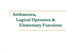
each ei can be considered as a conjecture of the learner regarding what the language L is, based on the data w0 , w1 , . . . , wi−1 . In general, the indices conjectured are from some index set J and interpreted in a hypothesis space {He : e ∈ J}, where {Le : e ∈ I} ⊆ {He : e ∈ J}. The learner maintains information about past data in form of some memory, which may change between cycles. Thus, the learner can be considered as an algorithmic mapping from (old memory, new datum) to (new memory, new conjecture) where the learner has some fixed initial memory. The learner learns or identifies the language L, if, for all possible texts for L, there is some k such that ek is an index for L and ek′ = ek for k′ ≥ k. The learner learns a class L of languages if it learns each language in L. The most basic set of hypothesis spaces are automatic families of languages. Here, a family of languages {Le : e ∈ I}, is automatic if the index set I and the set {conv(e, x) : e ∈ I, x ∈ Le } are both regular. Automatic families [18, 19] are the automata-theoretic counterpart of indexed families [1, 23] which were widely used in inductive inference to represent the class to be learnt. Note that when {Hd : d ∈ J} is a hypothesis space for {Le : e ∈ I}, which is an automatic family as well, then there is an automatic function f mapping the indices from J back to those in I, that is, Lf (d) = Hd for all those d ∈ J where Hd equals some Le . Hence one can without loss of generality (for learning criteria considered in this paper) directly use the hypothesis space {Le : e ∈ I} for the class {Le : e ∈ I} to be learnt. A learner M is called automatic if the mapping (old memory, new input word) to (new memory, new conjecture) for the learner is automatic, that is, the set {conv(om, dat, nm, nc) : M (om, dat) = (nm, nc)} is regular. In general, om and nm are the old and new versions of the long term memory of the learner. Automatic learners are, roughly speaking, the most restrictive form of learners which update a long term memory in each cycle where they process one new datum given to the learner. The next definition generalises the notion of automatic learning to a learner which has a linear or nearly linear time bound for each of its cycle. This generalisation is natural, due to the correspondence between automatic function and linear time computable functions given in the previous section of this paper. Definition 3.1. A learner M is a Turing machine which maintains some memory and in each cycle receives as input one word to be learnt, updates its memory and then outputs an hypothesis. The tapes of the Turing machine are all one-sided infinite and contain ⊞ at the left end. The machine operates in cycles, where in each cycle it reads one current datum (from a text of the language to be learnt) and formulates one hypothesis. Furthermore, it has some long term memory in its tape where the memory in Tape 0 is always there while the memories in the additional data structures (Tapes 1, 2, . . . , k) is only there when these additional data structures are explicitly permitted. • At the beginning of each cycle, Tape 0 (base tape) contains convolution of the input and some information (previous long term memory) which is not longer in length (up to an additive constant) than the length of the longest word seen so far. The head on Tape 0 of the Turing machine starts at ⊞ at the beginning of each cycle. • At the end of each cycle, Tape 0 (base tape) has to contain the convolution of the new long term memory and the hypothesis which the learner is conjecturing.


Base Tape

11

⊞ C C H C C ⊡

Work Tape 1 ⊞ C C C H C C C C C ⊡ ⊡ ⊡ . . . Work Tape 2 ⊞ C C C C C H C C C C ⊡ ⊡ . . . Figure 1: Learner with two working tapes; the head positions are H and other data positions are C; note that data characters can be convoluted characters from finitely many alphabets in order to store the convolution of several tracks on a tape. • During the execution of a cycle, the learner can run in time linear in the current length of Tape 0 and, like a position-faithful one-tape Turing machine, replace the convolution of the current datum and old long term memory by the convolution of the hypothesis and the new long term memory. Furthermore, the memory in Tape 0 has to meet the constraint that it is at most (up to an additive constant) the length of the longest datum seen so far (including the current datum), hence there is an explicit bound on the length of Tape 0 in each cycle. • Tapes 1, 2, . . . , k are normal tapes, whose contents and head positions are not modified during change of cycles. M can use these tapes for archiving information and doing calculations. There is no extra time allowance for the machine to use these tapes, hence the machine can only access a small amount (linear in the length of Tape 0) in each cycle of these tapes. • Without loss of generality, one can assume that the length of the longest datum seen so far is stored in the memory in Tape 0. The learner is said to have k additional work tapes iff it has in addition to Tape 0 also the Tapes 1, 2, . . . , k. Figure 1 illustrates a learner with two additional tapes. Note that in the definition of Tape 0, it is explicit that the length of the hypothesis produced is bounded by the length of the largest example seen so far plus a constant. This is compatible with learning, as for all automatic families, (i) for any finite set L in the family, the length of the smallest index e for L overshoots the length of the longest element of L by at most a constant and (ii) for any infinite set L in the family there are words in L which are longer than some index for L; thus a learner cannot fail just because the indices of a language Le are extremely long compared to the size of the members of Le – though, of course, there may be other reasons for a learner not to be successful. Note that if only Tape 0 is present, the model is equivalent to an automatic learner with the memory bounded by the size of the longest datum seen so far (plus a constant) [6, 18]. The next examples illustrate what type of learnable automatic classes exist. Example 3.2. The following automatic classes are learnable by an automatic learner with its memory bounded by the length of the longest example seen so far (plus a constant): First, the class of all extensions of an index, that is, I = Σ∗ and Le = e · Σ∗ for all e ∈ I. Here the learner maintains as a memory the longest common prefix e of all data seen so far and whenever the memory is e and a new datum x is processed, the learner updates e to the longest common prefix of both, e and x, which is also the next hypothesis. Second, the class of all closed intervals in the lexicographic ordering, that is, I = {conv(d, e) : d, e ∈ Σ∗ ∧ d ≤lex e} and Lconv(d,e) = {x ∈ Σ∗ : d ≤lex x ≤lex e}; here

12


x ≤lex y denotes that x is lexicographically before y. The learner maintains as memory the lexicographically least and greatest elements seen so far, the convolution of these elements also serves as hypothesis. Third, the class of all strings of length different from the index, that is, I = {0}∗ and Le = {x ∈ Σ∗ : |x| = 6 |e|}. Here the learner archives in Tape 0 binary string which is of length 1 plus the length of the longest example seen so far; the k-th bit of this string (starting with k = 0) is 1 iff an example of length k has been seen so far, and 0 iff no example of length k has been seen so far. The conjecture is 0h for the least h such that either the h-th bit of the memory is 0 or h is 1 plus the length of the memory string. For any automatic family, {He : e ∈ J}, the equivalence question for indices is automatic, that is, the set {conv(e, e′ ) : He = He′ } is regular. Thus for the purposes of this paper, one can take the hypothesis space to be one-one, that is, different indices represent different languages. In a one-one hypothesis space, the index e of a finite language Le has, up to an additive constant, the same length as the longest word in Le ; this follows easily from [19, Theorem 3.5]. This observation is crucial as otherwise the time-constraint on the learner would prevent the learner from eventually outputting the correct index; for infinite languages this is not a problem as the language must contain arbitrarily long words. Angluin [1] gave a characterisation when a class is learnable in general. This characterisation, adjusted to automatic families, says that a class is learnable iff, for every e ∈ I, there exists a finite set D ⊆ Le such that there is no d ∈ I with D ⊆ Ld ⊂ Le . All the automatic families from Example 3.2 satisfy this criterion; however, Gold [11] provided a simple example of a non-learnable class which of course then also fails at Angluin’s criterion: One infinite set plus all of its finite subsets. The main question of this section is which learnable classes can also be learnt by a linear-time learner with k additional work tapes. For k = 0, this is in general not possible, as automatic learners fail to learn various learnable classes [18], for example the class of all sets {0, 1}∗ − {x}, with the index x being from {0, 1}∗ , and the class of all sets Le = {x ∈ {0, 1}|e| : x 6= e}. Freivalds, Kinber and Smith [10] introduced limitations on the long term memory into inductive inference; Kinber and Stephan [22] transferred it to the field of language learning. Automatic learners have similar limitations and are therefore not able to learn all learnable automatic classes [6, 18]. The usage of additional work tapes for linear time learners permits to overcome these limitations, the next results specify how many additional work tapes are needed. Recall from above that work tapes are said to be additional iff they are in addition to the base tape. Theorem 3.3. Suppose Σ = {0, 1, 2} and consider the automatic family L over the alphabet Σ which is defined as follows: L consists of (i) Lε = {0, 1}∗ and (ii) Lx0 = {0, 1}∗ ∪ {x2} − {x} and (iii) Lx1 = {0, 1}∗ ∪{x2}, for each x ∈ {0, 1}∗ . Then, L does not have an automatic learner but has a linear-time learner using one additional work tape. Proof. An automatic learner cannot memorise all the data from {0, 1}∗ it sees. For any automatic learner, one can show, see [18], that there are two finite sequences of words from Lε , one containing x and one not containing x, such that the automatic learner has the same long term memory after having seen both sequences. If one presents to the automatic learner, after these sequences, all the elements of Lx0 , then the automatic learner’s limiting behaviour on the two texts so formed is the same, even though they are texts for two


13

different languages, Lx1 or Lx0 , in L. Therefore the learner cannot learn the class L. A linear time learner with one additional work tape (called Tape 1) initially conjectures Lε and uses Tape 1 to archive all the examples seen at the current end of the written part of the tape. When the learner sees a word of the form x2, it maintains a copy of it in the memory part of Tape 0 and conjectures x0 as its hypothesis. In each subsequent cycle, the learner scrolls back Tape 1 by one word and compares the word there as well as the current input with x2; if one of these two is x then the learner changes its conjecture to Lx1 , else it keeps its conjecture as Lx0 . In the case that the origin of Tape 1 (⊞) is reached, the learner from then onwards ignores Tape 1 and only compares the incoming input with x2. It is easy to verify that the learner as described above learns L. ✷ Theorem 3.4. Every learnable automatic family L has a linear-time learner using two additional work tapes. Proof. Jain, Luo and Stephan [18] showed that for every learnable automatic family L = {Le : e ∈ I} there is an automatic learner M using memory bounded in length by the length of the longest example seen so far (plus a constant) which learns the class from every fat text (a text in which every element of the language appears infinitely often). So the main idea is to use the two additional tapes in order to simulate and feed the learner M with a fat text. The two additional tapes are used to store all the incoming data and then to feed the learner M with each data item infinitely often. The words in the tapes are stored using some separator # to separate the words. Thus, 00#1##11⊡ indicates that the tape contains the words 00, 1, ε and 11. The learner N for L using two additional tapes works as follows. Suppose the previous memory stored in Tape 0 is memk (initially the memory stored on Tape 0 is the initial memory of M ) and the current datum is wk . Then, N does the following: • Compute M (memk , wk ) = (mem′ , e′ ). • Find the last word in Tape 1, say t. Erase this word from Tape 1. In the case that Tape 1 was already empty, let t = wk . • Compute M (mem′ , t) = (memk+1 , ek ). • Write wk and t at the end of Tape 2 (using the separator # to separate the words). • When the beginning of Tape 1 is reached (⊞), interchange the roles of Tape 1 and Tape 2 from the next cycle. • The new memory to be stored on Tape 0 is memk+1 and the conjecture is ek . It is easy to see that in each cycle, the time spent is proportional to |memk | + |wk | + |t| and thus linear in the length of the longest word seen so far (plus a constant); note that mem′ , e′ , ek are also bounded by that length (plus a constant). Furthermore, in the simulation of M , each input word to N is given to M infinitely often. Hence N learns each language from the class L. ✷ Open Problem 3.5. It is unknown whether one can learn every in principal learnable automatic class using an automatic learner augmented by only one work tape. Further investigations deal with the question what happens if one does not add further work tapes to the learner but uses other methods to store memory. Indeed, the organisation in a tape is a bit awkward and using a queue solves some problems. A queue is a tape where one reads at one end and writes at the opposite end, both the reading and writing heads are unidirectional and cannot overtake each other. Tape 0 satisfies the same constraints as

14


in the model of additional work tapes and one also has the constraint that in each cycle only linearly many symbols (measured in the length of the longest datum seen so far) are stored in the queue and retrieved from it. Theorem 3.6. Every learnable automatic family L has a linear-time learner using one additional queue as a data structure. Proof. The learner simulates an automatic learner M for L using fat text, in a way similar to that done in Theorem 3.4. Let M in the k-th step map (memk , wk ) to (memk+1 , ek ) for M ’s memory memk . For ease of presentation, the contents of Tape 0 is considered as consisting of a convolution of 4 items (rather than 2 items, as considered in other parts of the paper). At the beginning of a cycle the linear-time learner N has conv(vk , −, memk , −) on Tape 0 where vk is the current datum, memk the archived memory of M and “−” refers to irrelevant or empty content. In the k-th cycle, the linear-time learner N scans four times over Tape 0 from beginning to the end and each time afterwards returns to the beginning of the tape: (1) Copy vk from Tape 0 to the write-end of the queue; (2) Read a word from the read-end of the queue, call it wk , and update Tape 0 to conv(vk , wk , memk , −); (3) Copy wk from Tape 0 to the write-end of the queue; (4) Simulate M on Tape 0 in order to map (memk , wk ) to (memk+1 , ek ) and update Tape 0 to conv(vk , wk , memk+1 , ek ). It can easily be verified that this algorithm permits to simulate M using the data type of a queue and that each cycle takes only time linear in the length of the longest datum seen so far. Thus, N learns L. ✷ A further data structure investigated is the provision of additional stacks. Tape 0 remains a tape in this model and has still to obey to the resource-bound of not being longer than the longest word seen so far (plus a constant). Theorems 3.3 and 3.4 work also with one and two stacks, respectively, as the additional work tapes are actually used like stacks. Theorem 3.7. There is an automatic class which can be learnt with one additional stack but not by an automatic learner. Furthermore, every learnable automatic class can be learnt by a learner using two additional stacks. Furthermore, the next result shows that in general one stack is not enough; so one additional stack gives only intermediate learning power while two or more additional stacks give the full learning power. The class witnessing the separation contains only finite sets. For information on Kolmogorov complexity, the reader is referred to standard text books [5, 9, 24, 25]. The next paragraphs provide a brief description of the basic concepts. Consider a Turing machine U which computes a partial-recursive function from {0, 1}∗ × {0, 1}∗ to {0, 1}∗ . The first input to U is also referred to as a program. Machine U is universal iff for every further machine V , there is a constant c such that, for every (p, y) in the domain of V , there is a q, which is at most c symbols longer than p, satisfying U (q, y) = V (p, y). Fix a universal machine U . Now the conditional Kolmogorov complexity C(x|y) is the length of the shortest program p with U (p, y) = x; the plain Kolmogorov complexity C(x) is C(x|ε). Note that, due to the universality of U , the values of C(·) can only be improved by a constant (independent of x, y) when changing from one universal machine to another one. In some cases below, C(x|y1 , y2 , . . . , yr ) is the conditional Kolmogorov


15

complexity when given an r-tuple (y1 , y2 , . . . , yr ) where r might vary; such a tuple can be coded up in any way which permits to identify the parts uniquely, as automaticity is not required, the coding 0|y1 | 1y1 0|y2 | 1y2 . . . 0|yr | 1yr would do it. If f is a partial-recursive function then there is a constant c with C(f (x)|y) ≤ C(x|y)+c for all x in the domain of f . In particular, if one can find a way to describe the strings x in a set A by binary strings px such that some algorithm can compute each x ∈ A from the corresponding description px , then C(x) ≤ |px | + c for some constant c and all x ∈ A. For this reason, one often says that x can be described by n bits when the corresponding px can be chosen to have n bits. Theorem 3.8. The class of all Le = {x ∈ {0, 1}|e| : x 6= e} with e ∈ {0, 1}∗ ∪ {2}∗ cannot be learnt by a linear-time learner using one additional stack. Proof. Assume that the linear-time learner M using one stack, in addition to the base tape, is given. In order to find languages not learnt by M , one focuses on Le where the parameter n = |e| is large; in addition one considers only n of the form k + 2k for some k; this parameter k and m = 2k will play some role in the arguments below. Note that all data-items in Le have the length n. For i ∈ {1, 2, . . . , m}, let xi be a string of length n such that the Kolmogorov complexity C(x1 x2 . . . xm ) is at least (n − k)m and the first k bits of each xi is the binary bit representation of i − 1. Furthermore, assume that c is a constant so large that the Kolmogorov complexity of the content of Tape 0 (which can be assumed to be always n symbols long, since all data have length n, but which can use more than two alphabet symbols) is at most cn and that the stack can, in each round, pull or push up to cn symbols, where the stack alphabet has at most 2 symbols (one can code up a larger alphabet in binary and choose the constant c sufficiently large to absorb the extra amount of storage). Hence, in each cycle, what the machine does depends on the content of Tape 0 (worth cn bits) and on the top cn symbols of the stack (worth cn bits). Furthermore, assume that all words of length n different from x1 , x2 , . . . , xm have already been presented to the learner and let α denote the content of Tape 0 and uβ denote the content of the stack where β are the top cn symbols (or less if u is the empty word). Below one considers the behaviour/configuration of the learner when it is presented with further inputs and one considers (α, uβ) as the initial configuration of the learner for this purpose. Below, the configuration of the learner, at any stage before reading the next input, is denoted by (·, ·), where the first argument is the content of the tape and the second argument is the content of the stack. Intuitively, as the xj ’s are complex, the learner needs to store them on the stack when it receives them (otherwise, it would lose information about which xj ’s it has seen). This forces the stack to grow larger and larger and prevents the learner from accessing earlier stored data on the stack, thus making the earlier stored information useless. This allows to show that some language Le is not learnable by M . Claim 3.11 gives a permutation xi1 , xi2 , . . . , xim of x1 , x2 , . . . , xm such that M does not touch any, but the top 6(c + 1)2 n symbols of u, on input xi1 , xi2 , . . . , xim . Claim 3.12 uses this claim to show that on some sequence σ of xi ’s, M reaches a configuration (α′ , vw′ β ′ ), with |β ′ | = cn and v being same as u except for the top 6(c + 1)2 n symbols removed, where the learner never touches v on the input σ, and for any future input involving xi ’s never touches vw′ . This, then allows to claim in Claim 3.13 that the learner cannot learn some Le . Claims 3.9 and 3.10 are used in proving the above claims. Now the five claims about the configuration of M are proven formally.

16


Claim 3.9. There do not exist two distinct input sequences of words of length n, one containing an xi and one not containing xi , ending up in the same configuration (α′ , vβ ′ ) where β ′ has at most length cn and v has not been touched (that is, starting from configuration (α, uβ), the initial portion v of uβ above was never at the top of the stack during the processing of any of the two sequences). Assume by way of contradiction that this claim fails, that is, there are two such sequences σ and σ ′ . Then one can bring the learner into the configuration (α′ , vβ ′ ) by either of the sequences and thereafter feed the learner with the xj with j 6= i, and then with a string of length n, different from xi , forever. The convergence behaviour of the learner, in both cases, is the same as the configuration (α′ , vβ ′ ) is independent of the sequence σ or σ ′ by which the learner reached it; from then onwards the learner receives, in both cases, the same data and conjectures the same hypotheses, as in both cases they are based on the same data, Tape 0 and stack. In one case the learner has to learn Lxi = {0, 1}n − {xi } and in the other case the learner has to learn L2n = {0, 1}n ; thus the learner can learn at most one of these two sets. This completes the proof of the claim. Claim 3.10. There is no input sequence (xi1 , xi2 , . . . , xiℓ ) and no splitting of u into vw such that M , after reading these inputs, is in a configuration of the form (α′ , vβ ′ ) with |β ′ | ≤ cn and without having pulled and pushed back any symbols of v and with the conditional Kolmogorov complexity satisfying C(xi1 xi2 . . . xiℓ |α, wβ, i1 , i2 , . . . , iℓ ) ≥ (c + 1)2 n. For a proof of the claim, assume by way of contradiction that there is such an input sequence (xi1 , xi2 , . . . , xiℓ ). Then there is a partial-recursive function f such that f , given (α, wβ, i1 , i2 , . . . , iℓ , α′ , β ′ ), finds a sequence yi1 , yi2 , . . . , yiℓ such that yij = yij′ whenever ij = ij ′ , yij ∈ {0, 1}n for all j, yij having the first k bits being the binary representation of ij and M pulling on these inputs the symbols belonging to wβ without touching those of v and ending up in the configuration (α′ , vβ ′ ). Note that one does not need to know v for this search, hence the search depends only on the inputs given to f and returns an input sequence such that its Kolmogorov complexity given (α, wβ, i1 , i2 , . . . , iℓ ) is at most that of (α′ , β ′ ), that is, below (c + 1)2 n (assuming that n is sufficiently large). It follows that at least one yij differs from xij ; furthermore, no other yij′ can be equal to xij by the rules that each yij′ encodes ij ′ in the first k bits and equals to yij whenever ij ′ = ij . However, this would contradict Claim 3.9. This completes the proof of Claim 3.10. Claim 3.11. There is a permutation (xi1 , xi2 , . . . , xim ) of (x1 , x2 , . . . , xm ) such that the splitting vw = u with either |w| = 6(c + 1)3 n or |w| < 6(c + 1)3 n ∧ |v| = 0 satisfies that M on input (xi1 , xi2 , . . . , xim ) never touches the symbols in v. Let vw be the given splitting of u. If |w| < 6(c + 1)3 n then v is empty and nothing needs to be proven; thus assume that |w| = 6(c + 1)3 n. Now define yk = x1 x2 . . . xm and inductively for ℓ = k − 1, k − 2, . . . , 1, split yℓ+1 at the middle into two equal parts yℓ and zℓ (both of length 2ℓ n) such that C(yℓ |k, α, wβ) ≥ C(zℓ |k, α, wβ). Note that there is a unique permutation of the form (xi1 , xi2 , . . . , xim ) of (x1 , x2 , . . . , xm ) such that xi1 xi2 . . . xim = y1 z1 z2 . . . zk−1 . Note that i2 , i3 , . . . , im can be computed from i1 . Note that C(yk |k, α, wβ) ≥ (n − 2k)m (for k and n = k + 2k , m = 2k being sufficiently large) for the following reasons: C(yk ) ≥ (n − k)m; C(yk |k, α, wβ) ≥ C(yk ) − C((k, α, wβ)) − k; C(k, α, wβ) + k ≤ 8(c + 1)3 n ≤ km/2. By induction one can see that C(yℓ |k, α, wβ) ≥ (n − 2k)m · 2ℓ−k − k for all ℓ whenever


17

k, n are sufficiently large; note that yℓ is the more complex half of yℓ+1 and therefore has by induction hypothesis at least the complexity (n − 2k) · m · 2ℓ+1−k /2 − k/2 minus some constant which can be brought into the form (n − 2k)m · 2ℓ−k − k by assuming that k/2 is larger than the corresponding constant. Furthermore, the values i1 , i2 , . . . , im can be computed from k and i1 , hence one can represent i1 , i2 , . . . , ih by i1 and h and k. Hence C(yℓ |α, wβ, i1 , . . . , ih ) ≥ (n − 2k)m · 2ℓ−k − 5k for any h with 2ℓ ≤ h < 2ℓ+1 . There are two cases for each h with 2ℓ ≤ h < 2ℓ+1 : First, 3(c + 1)2 n > |yℓ |. Then h < 6(c + 1)2 and, on input (xi1 , xi2 , . . . , xih ), the learner can have pulled at most 6c(c + 1)2 n symbols from the stack; hence it has neither touched v nor the bottom cn symbols of w. Second, 3(c + 1)2 n ≤ |yℓ |. Then C(yℓ |α, wβ, k, i1 , i2 , . . . , ih ) ≥ (n − 2k)m · 2ℓ−k − 5k ≥ 3(c + 1)2 (n − 2k) − 5k > 2(c + 1)2 n. Assuming that k and n = 2k + k are sufficiently large, one obtains C(xi1 xi2 . . . xih |α, wβ, i1 , i2 , . . . , ih ) ≥ (c + 1)2 n. Thus, using Claim 3.10 it follows that for all h ∈ {6(c + 1)2 , 6(c + 1)2 + 1, . . . , m} there are at least cn symbols in the stack above v after reading xi1 , xi2 , . . . , xih . Hence, using above cases, one can conclude by induction on h that the symbols in v are not touched while processing the input (xi1 , xi2 , . . . , xim ). Claim 3.12. Split u into vw as in Claim 3.11. There is a sequence of all xi , perhaps with repetitions, such that after reading this sequence M is in a configuration (α′ , vw′ β ′ ), with |β ′ | = cn, such that for all further inputs from x1 , x2 , . . . , xm , M does not touch the symbols on the part of the stack denoted by vw′ . Assuming that this sequence does not exist, one could use the sequence given in Claim 3.11 to remain above v in the stack until all symbols are passed and then one could feed some sequence of xi until all but at most cn symbols above v are used up; that is, one would be in a configuration of the form (α′ , vβ ′ ) with |α′ | = n and |β ′ | ≤ cn. Hence one can, given (α, wβ) and (α′ , β ′ ) search a tuple (y1 , y2 , . . . , ym ) such that each yi starts with a binary number of length k representing i − 1 and each yi has n bits and there is a sequence of inputs drawn from this tuple on which the configuration of M with (α, vwβ) changes to (α′ , vβ ′ ) without touching v. The first tuple (y1 , y2 , . . . , ym ) of this type found by searching has Kolmogorov complexity at most 8(c + 1)3 n (obtained by coding the inputs k, α, wβ, α′ , β ′ and the routine for the search programme) which is less than (n − k)m, the lower bound on the Kolmogorov complexity of x1 x2 . . . xm , for sufficiently large k, m, n. Therefore some yi differs from xi and therefore one can reach the configuration (α′ , vβ ′ ) from (α, vwβ) by either having seen xi or not having seen xi . It follows from Claim 3.9 that this cannot occur, hence there is some minimal extension w′ β ′ of v such that |β ′ | = cn and when reading any sequence of the data x1 , x2 , . . . , xm after having reached the configuration (α′ , vw′ β ′ ), it will not touch vw′ in the stack, that is, all future activity depends only on α′ and β ′ . Claim 3.13. M fails to learn some language of the form {0, 1}n − {xi } or {0, 1}n . Let u, v, w, α, β, α′ , β ′ , w′ as in Claim 3.12. One can now show that there is a tuple (y1 , y2 , . . . , ym ) with |yi | = n and yi extending the k-bit representation of i − 1 such that

18


M when fed with some input-sequence taken from {y1 , y2 , . . . , ym } ends up in a configuration of the form (α′ , vw′′ β ′ ) without touching v and this configuration is computed from (α, wβ, α′ , β ′ ); as in Claim 3.12 one can argue that some yi 6= xi . Now one can feed all the xj 6= xi into M for the configurations (α′ , vw′ β ′ ) and (α′ , vw′′ β ′ ), respectively, for both in the same way and in a loop repeated forever. In both cases the learner M either converges to the same index or does not converge, but in one case the text which M has received is a text for {0, 1}n and in the other case it is a text for {0, 1}n − {xi }. Hence M fails to learn at least one of these two sets. ✷ 4. Relaxing the Timing Constraints In this section, it is investigated how the learning power improves if the severe restrictions on work Tape 0 or the computation time are a bit relaxed. The next result shows that, if one allows a bit more than just linear time, then one can learn, using one work tape, all learnable automatic classes of infinite languages. The result could even be transferred to families of arbitrary r.e. sets as the simulated learner is an arbitrary recursive learner. Intuitively, think of f in the following theorem as a slowly growing function. Theorem 4.1. Assume that {Le : e ∈ I} is an automatic family where every Le is infinite and M is a recursive learner which learns this family. Furthermore, assume that f, g are recursive functions with the property that f (n) ≥ m whenever n ≥ g(m) (so g is some type of inverse of f ). Then there is a learner N which learns the above family, using only one additional work tape, and satisfies the following constraint: if n is the length of the longest example seen so far, then only the cells number 1, 2, . . . , n of Tape 0 can be non-empty and the update time of N in the current cycle is O(n · f (n)). Proof. The main idea of the proof is that one constructs a learner which splits Tape 1 into four tracks for archivation; the learner usually uses Track 1; in irregular intervals, the learner returns from its current position to the origin of Tape 1 and uses Track 2 for archiving the examples which come up during this “return to the origin” until it reaches the old data on Tracks 2 and 3. When this happens, the old data found there consist only of words up to length m (where m is sufficiently small compared to the current word length n) and the learner can compress the data in Tracks 1, 2 and 3 into a list α (to be maintained on Tape 0); α will contain, for each word w up to length m occurring in the input, at most one copy (which gives a corresponding length bound on the length of α). Once the compression is completed, the learner returns to the forward mode using the one left over free track for this purpose. The key idea is to “space out” the visits to the origin such that, for m being the length of the longest datum seen up to the end of the last visit, m is so much smaller than the current n that 2m+1 · (m + 1) ≤ f (n); this allows all the data which was archived up to the end of the previous visit to be compressed into a string of length up to f (n) and the update of this compressed memory can, in each round, be done in time O(f (n) · n). The description below gives a more precise description of the update protocol. As the memory has only to be bounded by the length of the longest datum seen so far plus some constant, one can assume without loss of generality that n is at least 1. On Tape 0, as memory, the learner N archives the convolution of variables α, β, γ, e, 0m , 0n with the following meaning. • 0n represents in unary the length of the longest word seen so far and 0m is an old value of 0n ; initially m and n are 1 (not 0).


19

• The variable α is, during the runtime, only modified by appending symbols at the end and will in the limit consist of a one-one text of all the words occurring in the language to be learnt; the words on α are separated by a special character. For example, α = #00##0101#11111# would represent a beginning of a text consisting of 00, ε, 0101 and 11111. Furthermore, each of the words in α would be of length at most m. • The variable β is the current configuration of a computation to determine g(2m+1 ·(m+1)) (in unary); this configuration is updated whenever the length and time constraints permit and the next configuration is shorter than 0n , until the computation finishes. • The variable γ is a configuration of M , while processing the initial part α of a text for the input language; note that this configuration includes the memory of M and the portion of α it has read. In each cycle this configuration is updated by one more step of the computation, unless the input α is currently exhausted (that is, M would like to read a symbol which is not yet there) or the length of the configuration becomes longer than 0n . • The variable e is the last completed conjecture of M and updated whenever the configuration γ of M contains a new value to be output. In each cycle, the learner N would archive the current input x on the work tape at a position near to the current one (that is, the input position has to be reached in linear time) and N would furthermore update the values of β, γ, e, 0m , 0n on Tape 0 (α is updated only during some cycles, see below). In order to be able to save all required information on the work Tape 1, the tape content is modeled as having four tracks. Usually, only Track 1 is used for appending new information at the end of the tape and Track 4 is used for making sure that computations of the variables of Tape 0 meet the time-bound. Tracks 2 and 3 are used to store data during cycles when some special operations are needed to transfer data from Tape 1 to the memory α in Tape 0. Furthermore, initially m = 1. When β shows that the computation of g(2m+1 · (m + 1)) has terminated, and the observed examples are so long that n ≥ g(2m+1 · (m + 1)) then the learner enters the phase to do special operations (for next several cycles, as many as needed). Note that eventually this happens for every value of m, as the input language is infinite (assuming it is from L). In each cycle during this special phase, from its current position at the end of Tape 1 back to the origin ⊞, N will transfer/copy all stored words in Tape 1 of length at most m, which are not already in α, to α. During this process, the older words stored in Tracks 2 and 3 may be erased (but not lost, as they have already been copied to α, as each of them are of length at most m). The new input words received during this phase are copied in Tracks 2 and 3 (see below). Note that a concatenation of all words up to length m is at most 2m+1 · (m + 1) long (including separating symbols) and hence |α| ≤ 2m+1 · (m + 1) whenever α consists only of copies of words up to length m appearing in the language to be learnt and each such word appears at most once in α. Now, it is described how special operations are done in the special phases, see also Figure 2 for a rough summary of the handling of old and new data in each cycle. When going back on Tape 1, N will do the following for all words w archived in Tracks 1, 2, 3 starting from the current position up to |x| + 1 positions left of the current position (here one also considers w that might only partially overlap with the cells in positions between the current position and |x|+ 1 to the left of the current position; recall that x is the current input data to the learner): if |w| ≤ m then w is compared with all words in α and in the case that it does not coincide with any archived word in α, w# is appended at the end of α; note that all words archived in the Tracks 2 and 3 have at most the length m. For each word

20


Mode Usual Backward Special Forward Special Old Data Before — In Tracks 1, 2 and 3 In Tracks 1 and 2 Old Data After — Into Base Tape and Track 1 Remains unchanged New Data Into Track 1 Into Track 2 Into Track 3 Figure 2: Handling of data at head position of Tape 1. In backward special mode, old short data is recorded into the base tape and old long data remains in Track 1. w, this operation needs time O(|α| · |w|). Note that w has at most length m and α at most length 2m+1 · (m + 1), giving an overall bound of O(2m+1 · (m + 1) · |w|) for the processing of each word w. Furthermore, the concatenation of all these words archived one after another has length at most 3|x| + 3m; so one can conclude that the whole operation needs time O(2m+1 · (m + 1) · n) which is O(f (n) · n) as g(2m+1 · (m + 1)) ≤ n. Furthermore, all w in Tracks 2 and 3 overlapping with the space between the current position in Tape 1 and the cell at position |x| left of the current position before the start of the cycle are cleared away as these w all have at most the length m. After the clearance, x will be archived in Track 2 (where a special symbol outside the alphabet used for the archivation data is used to fill up blank spaces, if needed) and the current position moves by |x| + 1 to the left. This is done until the origin ⊞ is reached. At this point, Track 3 is empty and can be used to archive the incoming data in a similar way while the Turing machine moves back from ⊞ to end of used part of Tape 1. When returning to the usual archivation mode, m is updated to be the current value of n so that all words archived in Tracks 2 and 3 are again having at most length m. From then onwards, one waits until so much data has been observed such that the computation of g(2m+1 · (m + 1)) has terminated and gives a value below (the new value of) n. One can see from this description that, when learning an infinite language, eventually all words observed will be appended to α and M will be simulated on the resulting one-one text of the language to be learnt. Thus, M will eventually stabilise on some index e, which will be taken over as output when the corresponding computation has terminated and n is larger than |e|. This shows that N follows the simulated learner M and therefore N learns the class to be learnt. ✷ Pitt’s original result [28] on linear time learners did not measure the time in the size of the largest example seen so far, but in the size of the overall amount of examples seen so far. So the next two results deal with the question of the additional learning power provided by one work tape or one stack when the learner can use a Tape 0 of length n and run in time linear in n where n is logarithm of the number of data seen so far plus the length of the longest example seen so far; hence n increases, though slowly, when a datum is presented multiply. Note that in the proof of Theorem 4.1, the main reason to use infinite languages and strings of larger and larger length n, was to be able to transfer all stored data of length m onto α. This can also be done if instead of the length n, the unbounded growing number of examples seen so far is used as a parameter to allow the time needed to do the transfer (in which case additionally, one can make α a fat text). For this, one needs to keep track of some earlier maximal length m′ and number of items n′ (including counting the multiple copies, in case they are there) so that 2 · m′ · n′ bounds the overall length of all examples


21

stored in Tracks 2 and 3. When the number of examples seen so far, n, is larger than the current length of α plus 2 · m′ · n′ , one can then start going back, copying new data in Track 2 until one reaches the point where the earlier data in Tracks 2 and 3 are stored. At this point one moves all data in Tracks 2 and 3 to the end of α which is stored in Tape 0 and then starts moving forward on Tape 1 again, copying new data into Track 3 until one reaches the end of recorded part of all the tracks. At this point one can consider Track 1 and Track 2 as old recorded data (earlier roles played by Tracks 2 and 3) and continue recording data in Track 3 up to the point when the learner has seen enough examples so as to copy the data in Tracks 1 and 2 to Tape 0. Continuing in this way, one can copy all data to α in Tape 0 eventually and use the data in Tape 0 to simulate an automatic learner on fat text by cycling through the examples archived in α. This allows to show the following result; its proof is similar to Theorem 4.1 and the details are omitted. Theorem 4.2. Let n be the logarithm of the number of data seen so far plus the length of the longest example seen so far and consider a learner which can store in Tape 0 information of length n and can access one additional work tape, with update time in each cycle being linear in the corresponding n. Then such a learner can learn every learnable automatic family. The previous and the next result compute the parameter n of the update time and length of Tape 0 in the same way. While the previous result showed that one additional work tape is sufficient for full learning power under the corresponding linear time model, the next result shows that one additional stack is insufficient for full learning power. Theorem 4.3. Let n be the logarithm of the number of data seen so far plus the length of the longest example seen so far and consider a learner which can store in Tape 0 information of length n and can access one additional stack, with update time in each cycle being linear in the corresponding n. Then such a learner fails to learn the class L of all set Le = {0, 1}∗ − {e} where the indices e range over {0, 1}∗ . Proof. Assume by way of contradiction that such a learner M for L exists. Intuitively, the idea of the proof is that if the learner gets complex strings (relative to the position), then it has to store it in the stack. Thus, if it gets complex strings in odd positions of the text, and even positions of the text are filled with simple strings (to form a complete text for some target language), then the learner has to push (codings of) the complex strings on the stack and is not able to look at these pushed symbols in later computation. This allows to construct two such texts for different languages in the class on which eventually the learner behaves in the same way (see Claim 4.8, and then the arguments after this claim); thus the learner can learn at most one of these two sets. Claims 4.4 to 4.7 are combinatorial claims based on Kolmogorov complexity, needed for proving Claim 4.8. Now the formal proof is given. Let bin(m) denote the binary representation of m using log(m+2) bits where, for k ≥ 1, log(k) is the downrounded logarithm of base 2, that is, the maximal integer h with 2h ≤ k. Claim 4.4. Suppose σ and τ are two finite sequences over {0, 1}∗ such that range(σ) − range(τ ) 6= ∅, range(τ ) − range(σ) 6= ∅, and M has the same Tape 0 content and stack content after processing either σ or τ . Then, M does not learn L. To show the above claim, let w ∈ range(σ) − range(τ ) and w′ ∈ range(τ ) − range(σ). Let T ′ be a text for {0, 1}∗ − {w, w′ }. Then, M has the same convergence behaviour (that is it

22


either diverges or converges to the same conjecture) on texts σT ′ and τ T ′ , which are texts for Lw′ and Lw respectively. Thus, M fails to learn at least one of these languages and thus fails to learn L. This completes the proof of the claim. For any recursive text T of any language satisfying |T (m)| ≤ log(m + 2) for all m, define RT (using an oracle for the halting problem K) as follows: Let RT (2m) = T (m) and RT (2m + 1) be the string x of length 16(log(m + 2)) ending with bin(m)10log(m+2)−1 which maximises C(x|RT (0)#RT (1)# . . . #RT (2m)). Claim 4.5. Let T be a recursive text satisfying |T (m)| ≤ log(m + 2) for all m. Then the following statements hold: (a) RT (2j + 1) are pairwise distinct for different j; (b) For each m, RT (2m + 1) ∈ / {T (i) : i ≤ m2 }; (c) For each m, C(RT (2m + 1)|RT (0)#RT (1)# . . . #RT (2m)) ≥ 14 log(m + 2). Part (a) follows by definition. Part (b), follows by definition of RT (2m+1) and the fact that 16 log(m+2) > log(m2 +2). For part (c) note that there exists a string x of length 16 log(m+ 2), which ends in bin(m)10log(m+2)−1 , with Kolmogorov complexity (given RT (0)#RT (1)# . . . #RT (2m)) at least 14 log(m + 2). As RT (2m + 1) is most complex such string x, part (c) follows. Claim 4.6. There exists a constant c2 such that the following holds for m ≥ c2 . Suppose T is a recursive text satisfying |T (i)| ≤ log(i + 2) for all i. Then, C(RT (2m + 1)#RT (2m + 2) # . . . #RT (2m + 2k − 1)|RT (0)#RT (1)# . . . #RT (2m)) ≥ k · log(m + 2). To see that the claim holds, note that for some constant c1 , for all x, y ∈ {0, 1}∗ , σ ∈ {0, 1, #}∗ , C((x, y)|σ) ≥ C(x|σ) + C(y|σ#x) − c1 , see [24]. Thus, for all large enough m, C(RT (2m + 1)#RT (2m + 2)# . . . #RT (2m + 2k)|RT (0)#RT (1)# . . . #RT (2m)) ≥

i=m+k−1 X

[14 log(i + 2) − c1 ] ≥ k log(m + 2)

i=m

(where the second last inequality follows from Claim 4.5(c)). Let UiT and ViT denote the Tape 0 content and stack content of M after processing RT (0), RT (1), . . . , RT (2i). Claim 4.7. There exists a constant c3 such that, for m and k greater than c3 , with m + k ≤ m2 , the following holds. Suppose T is a recursive text satisfying |T (i)| ≤ log(i + 2) for all i. Furthermore suppose that T is computed by a program of Kolmogorov complexity less than 6 log(m + 2). Then, k log(m + 2) . 3 To show that the claim holds, suppose m is large enough as required for Claim 4.6. Suppose T |U T , V T , k) < k log(m+2) . Note that by Claim 4.5 (b), for i with m ≤ i < T , Vm+k C(Um+k m m 3 m + k, RT (2i + 1) does not belong to T (0), T (1), . . . , T (m + k). Now, given a program for T T , V T , k, U T T and Um m m+k , Vm+k , one can construct w2m+1 , w2m+3 , . . . , w2m+2k−1 such that, for i with m ≤ i < m + k, (i) w2i+1 ends in bin(i)10log(i+2) , (ii) w2i+1 ∈ / {T (0), T (1) . . . T (m + k)}, T T T )|(Um , VmT , k)) ≥ , Vm+k C((Um+k


23

T and stack content V T , on input sequence w (iii) M starting with Tape 0 content Um 2m+1 T (m+ m T and stack content 2)w2m+3 . . . w2m+2k−1 T (m + k), ends in Tape 0 content being Um+k T . Vm+k T and V T can be computed using R (0)#R (1)# . . . #R (2m). Thus, the Note that Um T T T m expression C(w2m+1 #RT (2m + 2)#w2m+3 #RT (2m + 4) . . . #w2m+2k−1 |RT (0)#RT (1) # . . . #RT (2m)) T T |U T , V T , k) + 2 log(k + 2) + 12 log(m + 2) + c′ ≤ k log(m+2) + is bounded by C(Um+k , Vm+k m m 3 2 log(k + 2) + 12 log(m + 2) + c′ for some constant c′ . However, by Claim 4.6, C((RT (2m + 1)#RT (2m + 2)# . . . #RT (2m + 2k − 1))|RT (0)#RT (1)# . . . #RT (2m)) ≥ k · log(m + 2). Thus, for large enough m, there are some h, w, w′ satisfying m ≤ h < m + k, w′ = w2h+1 6= w = RT (2h + 1) and w, w′ ∈ / {T (0), T (1), . . . , T (m + k)}. But, then by Claim 4.4 and T )|(U T , V T , k)) ≥ k·log(m+2) . This T , Vm+k Claim 4.5(a), M does not learn L. Hence, C((Um+k k k 3 proves Claim 4.7.

Claim 4.8. There exists a constant c5 such that for large enough m and m + k ≤ m2 the following holds. Suppose T is a recursive text satisfying |T (i)| ≤ log(i + 2) for all i, and T is computed by a program of Kolmogorov complexity less than 6 log(m + 2). Then, while processing RT (2m + 1)RT (2m + 2) . . . RT (2m + 2k), (a) the part of stack consisting of VmT , except for the top c5 log(m + 2) symbols, is never removed and T | ≥ (|V T | − c log(m + 2)) + k log(m+2) . (b) |Vm+k 5 m 4 T | = O(log(k + m + 2)), and thus To show the claim, consider k ≤ m2 − m. Now, |Uk+m T T T T C(Uk+m |Um , Vm , k) = O(log(k + m + 2)). Furthermore, if Vk+m = vw, for some longest T T prefix v of Vm , then the length of the deleted portion of Vm (that is |VkT |−|v|), can be at most k·log(k+m+2)·c′ , for a constant c′ ; this can be coded using log(k+2)+log log(k+m+2)+c′ bits. Hence, by Claim 4.7, for some constant c4 , |w| ≥ k·log(m+2) −c4 [log(m+2)+log(k+2)] ≥ 3 k·log(m+2) ′′ ′′ , for m, k ≥ c , for some constant c . Thus, for large enough k, the length of w 4 above is larger than what can be removed from the stack in one cycle. It follows that, for some constant c5 , the machine M , on input RT (2m + 1), RT (2m + 2), . . . , RT (2m + k), does not remove symbols from VmT , except maybe for up to c5 log(m + 2) symbols from the top. This proves part (a). Part (b) follows, by using the length of w above. This completes the proof of Claim 4.8. Using (a) and (b) of the above claim, it follows that for large enough m, for each recursive text T of some subset of {0, 1}∗ and T having a program shorter than 6 log(m + 2), M on RT (0), RT (1), . . . , RT (2m) will, when processing subsequent data from RT , never remove symbols from VmT except maybe for the top c5 · log(m + 2) symbols. T and the topmost Now, given a program for T , m, RT (0)#RT (1)# . . . #RT (2m), U2m T c5 · log(2m + 2) symbols of V2m , one can compute a sequence σ of length 4m + 1 such that, (i) σ(s) = RT (s), for s ≤ 2m, (ii) for all i ≤ 2m, σ(2i) = T (i) and (iii) for all i < 2m, σ(2i + 1) ends with bin(i)10log(i+2) and is of length 16 log(i + 2).

24


T and the top c log(2m + 2) symbols of (iv) M after processing σ has Tape 0 content U2m 5 T . the stack are same as the top c5 log(2m + 2) symbols of V2m Now, C(σ|RT (0)#RT (1)# . . . #RT (2m)), is at most c6 · log(m + 2), for some constant c6 , as it was constructed from a description of m and a description of the top c5 log(2m + 2) stack T . On the other hand, C(R (2m + 1)#R (2m + symbols and O(log(2m + 2)) symbols of U2m T T 2)# . . . #RT (2m + 2m)|RT (0)#RT (1)# . . . #RT (2m)) ≥ m · log(m + 2) by Claim 4.6. Hence, fix a text T = T0 of the nonempty strings which repeats each string infinitely often and let m be large enough and let σ be computed as above. It follows that σ and RT0 (0)RT0 (1) . . . RT0 (4m) differ for an i with m ≤ i < 2m, that is, satisfy σ(2i + 1) 6= RT0 (2i + 1). Let w = σ(2i + 1) and w′ = RT0 (2i + 1). The strings w, w′ do not occur in T0 (0)T0 (1) . . . T0 (m2 ). Let m′ and m′′ be least such that T0 (m′ ) = w and T0 (m′′ ) = w′ . Without loss of generality assume m′ < m′′ . Let T1 and T2 be obtained from T0 as follows: • If T0 (i) = T0 (m′ ) then T1 (i) = ε else T1 (i) = T0 (i); • If T1 (i) = T1 (m′′ ) then T2 (i) = ε else T2 (i) = T1 (i). Furthermore, the index of T1 has Kolmogorov complexity bounded by log(m′ + 2) and the index of T2 has Kolmogorov complexity bounded by 2 log(m′′ +2) up to an additive constant. When considering m (and thus m′ and m′′ ) large enough, one can absorb this constant into log(m′ + 2) and log(m′′ + 2) respectively, and thus Kolmogorov complexity of T1 and T2 are bounded by 3 log(m′′ + 2). Now RT1 coincides with RT0 below 2m′ , and RT2 coincides with RT1 below 2m′′ . In the various claims above (Claim 4.7, Claim 4.8), when using complexity of T being 6 log(m + 2), only the initial portion of text T of length at most m2 was used. Thus, it was enough to have the complexity of some text T ′ coinciding with T up to first m2 elements having a complexity below 6 log(m + 2). Hence, T1 and T2 satisfy the requirements needed in the claims. Thus, one can conclude that, when M processes text RT2 , for large enough s, the machine M (after having seen the first 2s + 1 elements of RT2 ) does not remove more than c5 · log(s + 2) symbols from the top of the stack VsT2 . Furthermore, if one now replaces the first 4m + 1 members of RT2 by the corresponding members of σ, then one gets that M on this new text RT′ 2 has the same convergence behaviour as on RT2 ; however, one text is for Lw while the other one is for Lw′ , thus these are texts for two different languages and so M does not learn at least one of these languages. ✷

5. Conclusion The starting point of this research is that automatic functions can be characterised using one-tape Turing machines. More precisely, a function is automatic iff it is computed by a position-faithful one-tape Turing machine in linear time. This is the smallest reasonable linear time complexity class and so the automatic functions turn out to sit at the bottom of the corresponding hierarchy. An open problem is whether the corresponding formalisation using alternating linear time position-faithful one-tape Turing machines also characterises the automatic functions. Automatic functions have been investigated in learning theory in order to model resourcebounded learners. Due to Pitt’s delaying trick [28], unrestricted recursive learners can be bounded heavily in the time that they use without losing learning power. However, automatic learners are not able to learn every learnable class, as their ability to memorise data


25

is insufficient. Therefore, one might ask whether one can replace an automatic learner by a linear-time learner working on a one-tape Turing machine with a tape of length bounded by the longest datum seen so far plus some additional memory. These additional memory devices are not restricted in length, though restricted in the amount of access the learner has per cycle: In each cycle the learner runs in time linear in the longest example seen so far, updates the base tape and accesses the additional storage devices only to retrieve or store a linear number of symbols. It is shown that two additional work tapes, two additional stacks or one additional queue give full learning power; furthermore, the learning power of one additional stack is properly intermediate and the learning power of one additional work tape is better than no additional work tape. It is an open problem whether there is a difference in the learning power of one and two additional work tapes. For some special cases and slightly superlinear computation time, it was possible to show that one additional work tape is enough. The methods of this proof do not generalise to the general case. References [1] Dana Angluin. Inductive inference of formal languages from positive data. Information and Control 45:117–135, 1980. [2] Lenore Blum and Manuel Blum. Toward a mathematical theory of inductive inference. Information and Control, 28:125–155, 1975. [3] Achim Blumensath. Automatic structures. Diploma thesis, Department of Computer Science, RWTH Aachen, 1999. [4] Achim Blumensath and Erich Gr¨ adel. Automatic structures. 15th Annual IEEE Symposium on Logic in Computer Science, LICS 2000, pages 51–62, 2000. [5] Cristian S. Calude. Information and Randomness: An Algorithmic Perspective. Second edition, Springer, Heidelberg, 2002. [6] John Case, Sanjay Jain, Trong Dao Le, Yuh Shin Ong, Pavel Semukhin and Frank Stephan. Automatic learning of subclasses of pattern languages. In Information and Comptation, Volume 218, pages 17–35, 2012. [7] John Case, Sanjay Jain and Frank Stephan. Automatic Functions, Linear Time and Learning. Computability in Europe: How the world computes – Turing Centenary Coference and Eighth Conference on Computability in Europe, (CiE) 2012. Springer LNCS: 7318: 96–106, 2012. [8] Ashok K. Chandra, Dexter C. Kozen and Larry J. Stockmeyer. Alternation. Journal of the ACM 28:114– 133, 1981. [9] Rodney G. Downey and Denis R. Hirschfeldt. Algorithmic Randomness and Complexity. Springer, Heidelberg, 2010. [10] R¯ usi¸ nˇs Freivalds, Efim Kinber and Carl H. Smith. On the impact of forgetting on learning machines. Journal of the ACM, 42:1146–1168, 1995. [11] E. Mark Gold. Language identification in the limit. Information and Control 10:447–474, 1967. [12] Juris Hartmanis. Computational complexity of one-tape Turing machine computations. Journal of the Association of Computing Machinery 15:411–418, 1968. [13] Fred C. Hennie. Crossing sequences and off-line Turing machine computations. Sixth Annual Symposium on Switching Circuit Theory and Logical Design, pages 168–172, 1965. [14] Fred C. Hennie. One-tape, off-line Turing machine computations. Information and Control 8:553–578, 1965. [15] Bernard R. Hodgson. Théories décidables par automate fini. Ph.D. thesis, Département de mathématiques et de statistique, Université de Montréal, 1976. [16] Bernard R. Hodgson. Décidabilité par automate fini. Annales des sciences mathématiques du Québec, 7(1):39–57, 1983.

26


[17] John E. Hopcroft, Rajeev Motwani and Jeffrey D. Ullman. Introduction to Automata Theory, Languages, and Computation. Second Edition, Addison-Wesley, 2001. [18] Sanjay Jain, Qinglong Luo and Frank Stephan. Learnability of automatic classes. Language and Automata Theory and Applications, 4th International Conference, LATA 2010. Proceedings. Springer LNCS 6031:321-332, 2010. [19] Sanjay Jain, Yuh Shin Ong, Shi Pu and Frank Stephan. On automatic families. Proceedings of the eleventh Asian Logic Conference in honour of Professor Chong Chitat on his sixtieth birthday, pages 94–113, World Scientific, 2012. [20] Sanjay Jain, Daniel N. Osherson, James S. Royer and Arun Sharma. Systems That Learn. MIT Press, Second Edition, 1999. [21] Bakhadyr Khoussainov and Anil Nerode. Automatic presentations of structures. Logical and Computational Complexity, (International Workshop LCC 1994). Springer LNCS 960:367–392, 1995. [22] Efim Kinber and Frank Stephan. Language learning from texts: mind changes, limited memory and monotonicity. Information and Computation, 123:224–241, 1995. [23] Steffen Lange, Thomas Zeugmann and Sandra Zilles. Learning indexed families of recursive languages from positive data: a survey. Theoretical Computer Science, 397:194–232, 2008. [24] Ming Li and Paul Vit´ anyi. An Introduction to Kolmogorov Complexity and its Applications. Third Edition. Springer, 2008. [25] André Nies. Computability and Randomness. Volume 51 of Oxford Logic Guides. Oxford University Press, Oxford, 2009. [26] Piergiorgio Odifreddi. Classical Recursion Theory, Volume II. Studies in Logic and the Foundations of Mathematics, 143. Elsevier, 1999. [27] Daniel Osherson, Michael Stob and Scott Weinstein. Systems That Learn, An Introduction to Learning Theory for Cognitive and Computer Scientists. Bradford — The MIT Press, Cambridge, Massachusetts, 1986. [28] Lenny Pitt. Inductive inference, DFAs, and computational complexity. Analogical and Inductive Inference, Proceedings of the Second International Workshop, AII 1989. Springer LNAI 397:18–44, 1989. [29] Sasha Rubin. Automata presenting structures: a survey of the finite string case. The Bulletin of Symbolic Logic, 14:169–209, 2008. [30] Boris A. Trakhtenbrot. Turing computations with logarithmic delay. Algebra i Logika, 3:33-48, 1964.

This work is licensed under the Creative Commons Attribution-NoDerivs License. To view a copy of this license, visit http://creativecommons.org/licenses/by-nd/2.0/ or send a letter to Creative Commons, 171 Second St, Suite 300, San Francisco, CA 94105, USA, or Eisenacher Strasse 2, 10777 Berlin, Germany

automatic functions, linear time and learning - Logical Methods in ...

automatic functions, linear time and learning - Logical Methods in ...

Suggest Documents

Linear and non-linear methods for automatic ... - Semantic Scholar

Linear Vs non-linear learning methods - arima

Automatic Control 1 - Continuous-time linear systems

Arithmetics, Logical Operators & Elementary Functions

Machine Learning Methods for Fully Automatic ... - CiteSeerX

Linear Combinations of Space-Time Covariance Functions and ...

The Automatic Synthesis of Linear Ranking Functions - BUGSENG

Grundy Functions and Linear Games

Linear time relational prototype based learning

DGTD methods using modal basis functions and symplectic local time

Linear Learning and Collaborative Learning

Mathematical Methods wk 4: Linear Operators on Functions

Logical Time in Model-Driven Engineering

Logical-And-Relational-Learning-Cognitive-Technologies.pdf ...

THE LOGICAL CATEGORIES OF LEARNING AND COMMUNICATION ...

Automatic Model Selection for Linear Time-Invariant Systems ...

Learning to Graph Linear Functions: A Case Study of Conceptual ...

for propositional and predicate logic - Logical Methods in Computer ...

Algorithms for Automatic Generation of Logical ... - ScienceDirect

Logical-And-Relational-Learning-Cognitive-Technologies.pdf ...

THE LOGICAL CATEGORIES OF LEARNING AND COMMUNICATION ...

Embedding time granularity in logical specifications of real-time systems

Learning Non-linear Ranking Functions for Web Search using ...

LOGICAL CHARACTERISATIONS OF INDUCTIVE LEARNING