Samizdat Press, Golden, Colorado (1997). 2. Gavalas, G.R., Shah, P.C., and Seinfeld, J.H.: âReservoir History Matching by. Bayesian Estimation,â paper SPE ...
AUTOMATIC HISTORY MATCHING IN BAYESIAN FRAMEWORK FOR FIELD-SCALE APPLICATIONS
A Dissertation by AHMED MOHAMED IBRAHIM DAOUD
Submitted to the Office of Graduate Studies of Texas A&M University in partial fulfillment of the requirements for the degree of DOCTOR OF PHILOSOPHY
December 2004
Major Subject: Petroleum Engineering
AUTOMATIC HISTORY MATCHING IN BAYESIAN FRAMEWORK FOR FIELD-SCALE APPLICATIONS
A Dissertation by AHMED MOHAMED IBRAHIM DAOUD
Submitted to Texas A&M University in partial fulfillment of the requirements for the degree of DOCTOR OF PHILOSOPHY
Approved as to style and content by: _______________________________ Akhil Datta-Gupta (Chair of Committee)
_______________________________ Daulat D. Mamora (Member)
_______________________________ Duane A. McVay (Member)
_______________________________ Yalchin R. Efendiev (Member)
_______________________________ Steve A. Holditch (Head of Department)
December 2004 Major Subject: Petroleum Engineering
iii
ABSTRACT
Automatic History Matching in Bayesian Framework for Field-Scale Applications. (December 2004) Ahmed Mohamed Ibrahim Daoud, B.S., Cairo University, Egypt; M.S., Cairo University, Egypt Chair of Advisory Committee: Dr. Akhil Datta-Gupta Conditioning geologic models to production data and assessment of uncertainty is generally done in a Bayesian framework. The current Bayesian approach suffers from three major limitations that make it impractical for field-scale applications. These are: first, the CPU time scaling behavior of the Bayesian inverse problem using the modified Gauss-Newton algorithm with full covariance as regularization behaves quadratically with increasing model size; second, the sensitivity calculation using finite difference as the forward model depends upon the number of model parameters or the number of data points; and third, the high CPU time and memory required for covariance matrix calculation. Different attempts were used to alleviate the third limitation by using analytically-derived stencil, but these are limited to the exponential models only. We propose a fast and robust adaptation of the Bayesian formulation for inverse modeling that overcomes many of the current limitations. First, we use a commercial finite difference simulator, ECLIPSE, as a forward model, which is general and can account for complex physical behavior that dominates most field applications. Second, the production data misfit is represented by a single generalized travel time misfit per well, thus effectively reducing the number of data points into one per well and ensuring the matching of the entire production history. Third, we use both the adjoint method and streamline-based sensitivity method for sensitivity calculations. The adjoint method depends on the number of wells integrated, and generally is of an order of magnitude less than the number of data points or the model parameters. The streamline method is more efficient and faster as it requires only one simulation run per iteration regardless of
iv
the number of model parameters or the data points. Fourth, for solving the inverse problem, we utilize an iterative sparse matrix solver, LSQR, along with an approximation of the square root of the inverse of the covariance calculated using a numerically-derived stencil, which is broadly applicable to a wide class of covariance models. Our proposed approach is computationally efficient and, more importantly, the CPU time scales linearly with respect to model size. This makes automatic history matching and uncertainty assessment using a Bayesian framework more feasible for large-scale applications. We demonstrate the power and utility of our approach using synthetic cases and a field example. The field example is from Goldsmith San Andres Unit in West Texas, where we matched 20 years of production history and generated multiple realizations using the Randomized Maximum Likelihood method for uncertainty assessment. Both the adjoint method and the streamline-based sensitivity method are used to illustrate the broad applicability of our approach.
v
DEDICATION
To my dear wife, to the soul of my mother, to my beloved father, to my brother, and to everyone who taught me a letter in my life.
vi
ACKNOWLEDGMENTS
First of all, I would like to express my endless thanks to God, ALLAH, for providing me with patience and help in performing this work. I would like to express my deep gratitude to my graduate advisor, Dr. Akhil DattaGupta, for his financial support, accessibility for discussion and academic guidance. I would like to thank Dr. Daulat D. Mamora, Dr. Duane A. McVay, and Dr. Yalchin R. Efendiev for serving as committee members. I acknowledge their helpful comments and suggestions. I wish to take this opportunity to extend my deep appreciation to Dr. Duane A. McVay and Chile Ogele for the work we have done together concerning integration and uncertainty quantification of volumetric and material balance analysis in Bayesian framework. Many thanks are due to Nayyar Sualehi and David Hammock for their help and guidance during my summer internship with Schlumberger Product Center, formation evaluation department. My cordial thanks are due to Dr. Younes Jalali for sharing his profound knowledge and experience with me and giving me the opportunity to work with his team last summer in Schlumberger well completion and productivity. I highly acknowledge the valuable guidance from Dr. Zhan Wu (now at UT-Austin) during my early work in adjoint method-based sensitivity. I want to thank my friends in the reservoir characterization group, Dr. Adel Malallah (now with Kuwait University), Dr. Sang Heon Lee (now with Chevron Texaco), Dr. Zhong He (now with Schlumberger), Dr. Arun Kharghoria (now with Petrotel), Dr. Leonardo Vega (now with Schlumberger), Harshal Parikh (now with Intera Inc.), Kamran Sabir (now with Aramco), Ahmed Al-Hutheli (now with Saudi Aramco), Danny Rojas, Hector Perez (now with Ecopetrol), Ill Nam, Mishal Al-Harbi, Ichiro Osako, Hao Cheng, Dayo Oyerinde, Eduardo Jimenez, Fady Chaban, Deepak Devegowda, Chengwu Yuan, and Xianlin Ma for helpful discussions, and for making my graduate years enjoyable and memorable.
vii
I would like to acknowledge financial support from the Joint Industry Project members. The facilities and resources provided by the Petroleum Engineering Department, Texas A&M University, are gratefully acknowledged. Last but not least, my sincere gratitude is to my beloved wife, Rania Rashad, for her continuous support and patience during my study at Texas A&M.
viii
TABLE OF CONTENTS Page ABSTRACT ....................................................................................................................iii DEDICATION ................................................................................................................. v ACKNOWLEDGMENTS............................................................................................... vi TABLE OF CONTENTS ..............................................................................................viii LIST OF TABLES .......................................................................................................... xi LIST OF FIGURES........................................................................................................ xii CHAPTER I
INTRODUCTION .......................................................................................... 1 1.1 Introduction ........................................................................................ 1 1.2 Literature Review............................................................................... 2 1.3 Objectives........................................................................................... 8 1.4 Dissertation Outline............................................................................ 9
II
BAYES THEORY AS A TOOL FOR DATA INTEGRATION AND UNCERTAINTY ASSESSMENT ............................................................... 11 2.1 Bayes Theory Background ............................................................... 11 2.2 Data Misfit........................................................................................ 13 2.2.1 Types of Data Misfit ............................................................... 13 2.2.2 Generalized Travel Time Formulation .................................... 17 2.3 Prior Model ...................................................................................... 20 2.4 Optimization Algorithms.................................................................. 21 2.4.1 Newton Algorithm................................................................... 21 2.4.2 Gauss-Newton Algorithm ....................................................... 23 2.4.3 Levenberg-Marquardt Algorithm............................................ 24 2.5 Bayesian Formulation for Field-Scale Applications ........................ 25 2.5.1 Bayesian Formulation ............................................................. 25 2.5.2 Square Root of the Inverse of the Covariance Using Numerically-Derived Stencil................................................... 28 2.5.3 Computation Scaling Properties: Conventional vs Field-Scale Bayesian Formulation..................................... 31 2.6 Bayesian Approach as a Tool for Uncertainty Assessment ............. 36
ix
CHAPTER
Page 2.6.1 Markov Chain Monte Carlo (MCMC) ................................... 37 2.6.2 Randomized Maximum Likelihood (RML) ............................ 38 2.7 Chapter Summary............................................................................. 39
III
SENSITIVITY COMPUTATION USING FINITE DIFFERENCE MODELS ..................................................................................................... 41 3.1 Adjoint Method-Based Sensitivity ................................................... 41 3.1.1 Forward Model Formulation ................................................... 42 3.1.2 Adjoint System Formulation ................................................... 44 3.1.2.1 Adjoint System Formulation in i,j,k Notation............. 53 3.1.3 Sensitivity Coefficients Formulation ...................................... 57 3.1.3.1 Sensitivity Coefficients Formulation in i,j,k Notation...................................................................... 59 3.2 Streamline-Based Sensitivity ........................................................... 61 3.2.1 Generalized Travel Time Sensitivity without Pressure Update ..................................................................................... 62 3.2.2 Generalized Travel Time Sensitivity with Pressure Update ... 66 3.3 Chapter Summary............................................................................. 66
IV
APPLICATIONS ......................................................................................... 68 4.1 Sensitivity Comparison .................................................................... 71 4.2 Synthetic Examples Using Adjoint Method-Based Sensitivity........ 75 4.2.1 Example 1: Reservoir of Three Permeability Regions............ 75 4.2.2 Example 2: Heterogeneous Reservoir ..................................... 83 4.3 Scaling Comparison ......................................................................... 90 4.4 Field Application: Goldsmith San Andreas Unit ............................. 94 4.4.1 Field Application: Adjoint Method-Based Sensitivity with Field-Scale Bayesian Approach ...................................... 98 4.4.2 Field Application: Streamline-Based Sensitivity with Field-Scale Bayesian Approach ................................... 101 4.5 Multiple Realizations from Posterior Distribution for Uncertainty Assessment: Goldsmith Field Application ................. 104 4.6 Chapter Summary........................................................................... 112
V
CONCLUSIONS AND RECOMMENDATIONS..................................... 114 5.1 Conclusions .................................................................................... 114 5.2 Recommendations .......................................................................... 117
NOMENCLATURE..................................................................................................... 121
x
Page REFERENCES............................................................................................................. 125 APPENDIX A .............................................................................................................. 131 APPENDIX B .............................................................................................................. 136 APPENDIX C .............................................................................................................. 152 VITA ............................................................................................................................ 163
xi
LIST OF TABLES
TABLE
Page
2.1 Location of the numerical stencil terms from column 63 of square root of inverse of covariance of 5 × 5 × 5 grid………………………………. 31 4.1 Data for example 1………………………………………………….....
76
4.2 Grid block size for the synthetic cases………………………………...
90
xii
LIST OF FIGURES
FIGURE
Page
2.1 Illustration of different types of data misfit, (a) Amplitude misfit, (b) Travel time misfit, (c) & (d) Generalized travel time misfit…………. 14 2.2 Illustration for the formulation of generalized travel time shift, (a) Shifting the calculated towards the observed: calculated to the right of the observed, (b) Shifting the calculated towards the observed: calculated to the left of the observed, (c) Shifting the observed towards the calculated: calculated to the right of the observed, (d) Shifting the observed towards the calculated: calculated to the left of the observed…………………………………………………………. 18 2.3 5x5x5 stencil used for the numerical approximation of the square root of the inverse of the covariance…………………………………. 30 2.4 Computational scaling for field-scale Bayesian vs conventional Bayesian……………………………………………………………… 35 4.1 Flowchart for automatic history matching process using adjoint method- based sensitivity…………………………………………….. 69 4.2 Flowchart for automatic history matching process using streamlinebased sensitivity……………………………………………………… 70 4.3 Comparison of travel time sensitivity with respect to horizontal permeability from the two layers, (a) perturbation, (b) Adjoint method. 74 4.4 Relative permeability data for example 1…………………………….. 76 4.5 (a) True permeability, (b) Initial and prior mean permeability for example 1…………………………………………………………….. 77 4.6 (a) Final permeability using conventional Bayesian approach, (b) True permeability for example 1………………………………..... 77 4.7 Water cut match for the four producers using conventional Bayesian approach for example 1………………………………………………. 78
xiii
FIGURE
Page
4.8 Misfit reduction for example 1 using conventional Bayesian approach……………………………………………………………... 78 4.9 Comparison between the exact covariance and covariance from 5x5x5 stencil at row 225 for example 1 ……………………………... 80 4.10 (a) Final permeability using field-scale Bayesian approach, (b) True permeability for example 1……………………………….... 81 4.11 Water cut match for the four producers using field-scale Bayesian approach for example 1……………………………………………... 81 4.12 Misfit reduction for example 1 using field-scale Bayesian approach……………………………………………………………... 82 4.13 (a) True permeability, (b) Initial and prior mean permeability for example 2…………………………………………………………….. 84 4.14 (a) Final permeability using conventional Bayesian approach, (b) True permeability for example 2……………………………….... 84 4.15 Water cut match for the four producers using conventional Bayesian approach for example 2………………………………………………. 85 4.16 Misfit reduction for example 2 using conventional Bayesian approach……………………………………………………………... 85 4.17 Comparison between the exact covariance and covariance from 5x5x5 stencil at row number 338 for example 2…………………….. 87 4.18 (a) Final permeability using field-scale Bayesian approach, (b) True permeability for example 2………………………………… 88 4.19 Water cut match for the four producers using field-scale Bayesian approach for example 2……………………………………………... 88 4.20 Misfit reduction for example 2 using field-scale Bayesian approach……………………………………………………………... 89 4.21 Well configuration for the synthetic examples, showing the location of the producers, the injectors and the producers whose water cut are 91 integrated during the history matching………………………………
xiv
FIGURE
Page
4.22 CPU time comparison during the minimization process between the conventional and field-scale Bayesian……………………………….. 92 4.23 CPU time comparison for sensitivity calculation between the adjoint method and streamline-based sensitivity…………………................... 93 4.24 CPU time per iteration for the whole inversion process for (a) adjoint method-based sensitivity; (b) streamline-based sensitivity................... 94 4.25 Goldsmith field – Co2 pilot project area………………………………
96
4.26 Well configuration of Goldsmith case study area……………………
96
4.27 Goldsmith field - porosity distribution……………………………….. 97 4.28 Initial and the prior mean permeability for Goldsmith case in log scale…………………………………………………………………... 97 4.29 Comparison between exact covariance and covariance from 5x5x5 stencil at row 15370 for Goldsmith case…………………………….. 97 4.30 Water cut match for Goldsmith case using adjoint method-based sensitivity, (a) Match from initial permeability model, (b) Match 99 from the final permeability model……………………………………. 4.31 (a) Final permeability, (b) permeability changes from initial (in Log scale) using adjoint method-based sensitivity……………………….. 100 4.32 Amplitude and generalized travel time misfit reduction using adjoint method-based sensitivity for Goldsmith case………………………… 100 4.33 Water cut match for Goldsmith case using streamline-based sensitivity, (a) Match from initial permeability model, (b) Match 102 from the final permeability model……………………………………. 4.34 Permeability changes from initial (in Log scale) using streamlinebased sensitivity……………………………………………………… 103 4.35 Amplitude and generalized travel time misfit reduction using streamline-based sensitivity for Goldsmith case……………………... 103
xv
FIGURE
Page
4.36 Permeability field, realization 1. (a) Unconditioned, (b)Conditioned, (c) Different. (Five out of ten layers, all in log scale)………………... 106 4.37 Permeability field, realization 2. (a) Unconditioned, (b)Conditioned, (c) Different. (Five out of ten layers, all in log scale)………………... 106 4.38 Permeability field, realization 3. (a) Unconditioned, (b)Conditioned, 107 (c) Different. (Five out of ten layers, all in log scale)……………… 4.39 Permeability field, realization 4. (a) Unconditioned, (b)Conditioned, (c) Different. (Five out of ten layers, all in log scale)………………... 107 4.40 Water cut, well 1. (a) Unconditioned, (b) Conditioned……………..
108
4.41 Water cut, well 2. (a) Unconditioned, (b) Conditioned……………..
108
4.42 Water Cut, Well 3. (a) Unconditioned, (b) Conditioned…………….. 109 4.43 Water cut, well 4. (a) Unconditioned, (b) Conditioned……………..
109
4.44 Water cut, well 5. (a) Unconditioned, (b) Conditioned……………..
110
4.45 Water cut, well 6. (a) Unconditioned, (b) Conditioned……………..
110
4.46 Water cut, well 7. (a) Unconditioned, (b) Conditioned……………..
111
4.47 Water cut, well 8. (a) Unconditioned, (b) Conditioned……………..
111
4.48 Water cut, well 9. (a) Unconditioned, (b) Conditioned……………..
112
1
CHAPTER I INTRODUCTION 1.1
Introduction
Automatic history matching is to find the best model parameters that minimize the error between the observed data and that calculated from the model without significant manual intervention. However, to do that there will be three major questions that we should answer.1 The first question is how accurate is the observed data that we need to match, the second one is how accurate is the forward model response, in other words, does the forward model include all the physics of the problem or not. The last one is that we can find an infinite number of model parameters that can fit the observed data, so which one to select, in other words, what is the prior information about the model parameters that are independent of the data observed. Here comes the important of the statistics to quantify the uncertainties in both the model and the data and the importance of Bayes’ theory (1763) to get the model that honor both the prior information about the model parameter and at the same time honor the data. In petroleum reservoir engineering the main objective is to build a reservoir model that honors both the geological information and the production history of the reservoir. The conventional method to do so is the manual history matching process which involves changing some parameters manually to get a good match with the production history. The selection of this parameter is subjective and always depends upon the engineering sense. This process is very tedious and time consuming; the alternative is using the automatic history-matching concept. The concept of the automatic history matching under Bayes theory is based on selecting a Gaussian probability distribution for the prior model parameter and a Gaussian distribution of the error in the data required to being matched. The dissertation follows the style and format of SPE Journal.
2
Then using Bayes theory, we get the posterior distribution that honors both the uncertainty of the prior and the data error. The model parameter can be permeability or porosity or skin factor or relative permeability or all of them and the data to be matched might be gas oil ratio, water cut, bottom-hole pressure or rate or all of them. The model parameter that maximizes the posterior distribution is the model parameter that honors both the data and the prior information. The framework of this study is to get the best permeability realization that honors both the prior information about the permeability distribution in the reservoir and the production history using Bayesian formulation. 1.2
Literature Review
Conditioning geological models to production data typically requires the solution of an inverse problem. Such inverse problems are usually ill-posed and their solutions suffer from difficulties in existence, uniqueness, and stability. To remedy these problems, a regularization term, in the form of data-independent prior information is generally added to the objective function in the inverse problem. Two different approaches to incorporate the regularization term have been used extensively in reservoir characterization literatures. One of these approaches is the Bayesian2-8, and the other is the deterministic.9-12 Both approaches have been successfully applied for conditioning geological models to production history and comparison between the two approaches can be found in the literature.13,14 Unlike the deterministic approach, the Bayesian approach associates probability distribution to the prior models and is thus considered well-suited for post-data inference and uncertainty assessment by defining a posterior distribution of models and sampling multiple realizations from this distribution. That is why Bayesian approach is commonly used for uncertainty assessment during production forecasting. Typically any inverse problem requires an optimization algorithm. These optimization algorithms can be classified into gradient-based and gradient-free algorithm. The gradient-free algorithms like simulated annealing or genetic algorithms
3
are not competitive with the gradient-based algorithm and computationally prohibitive for large-scale field applications. For the gradient-based algorithms, it is classified according to its search direction15 into steepest descent, Newton, quasi-Newton, and conjugate gradient. The fastest among those are the Newton-type search as it has a quadratic rate of convergence in the vicinity of the solution compared to the quasiNewton method which has a super linear rate of convergence, conjugate gradient and steepest descent which have linear rate of convergence and can be very slow in difficult problems. As Gauss-Newton and Levenberg-Marquard15 are considered one of the Newton-type of search algorithms, they are commonly used to get the maximum a posteriori estimate (MAP) from the posterior distribution by knowing the sensitivity coefficients which measure the change in the production response due to the change in the model parameters. As calculation of sensitivity is considered the key step in conditioning geologic model to production data, most of the literature survey work is focusing on the different approaches used for sensitivity computation. Jacquard and Jain16 presented an analytical formula for the sensitivity of pressure to a small perturbation in a uniform permeability field which depends on the number of wells and required about 1+Nw (Nw is the number of wells) simulation runs. Their method based on the assumptions of reciprocity theory and the linear relationship between the model parameters and the production response. Jacquard and Jain16 constructed estimates of two-dimensional permeability fields by history–matching single-phase flow pressure data by minimizing an objective function equal to the sum of squared pressure data mismatch terms. They used less than twenty parameters and they used an optimization procedure similar in spirit to the Levenberg-Marquardt algorithm to avoid the numerical instabilities that can arise when solving an ill-conditioned inverse problem. Jahns17 adapted the basic ideas of Jacquard and Jain16 to estimate both transmissibility and storage fields by matching single-phase flow pressure data. Jahns17 used the perturbation method which requires M+1 (M is the number of the model parameters) simulation runs to construct the sensitivities required by Gauss-Newton optimization algorithm and he shows that his method is computationally efficient
4
compared to Jacquard and Jain’s when the number of parameters is less than twice the number of wells. Jahns17 during inversion applies a sequence of minimization starting from small number of parameters to a bigger one (coarse to fine scale inversion). After about ten years of the fundamental work discussed in the previous paragraph, Carter et al.18 published a mathematical derivation of an efficient method to calculate sensitivity coefficients based on Jacquard and Jain’s16 method 18
simulation runs for sensitivity computation. Carter et al.
that require 1+Nw
considered 2D single-phase
flow problems with the same assumptions of Jacquard and Jain16. Their procedure gives the sensitivity of reservoir simulator grid block pressures to grid block transmissibility and storage. He et al.19 extended Carter et al.18 method for 3D single phase flow by estimating the sensitivity of the wellbore pressure with respect to the model parameter by using Peacman20 equation and a straightforward extension of Carter et al. sensitivities of grid block pressure with respect to the model parameters. The extension of Carter el al.18 method for 3D single phase reservoir models require a number of simulation runs equivalent to the number of the grid blocks penetrated by the well. However He et al.19 developed an approximate procedure to estimate the sensitivity of the wellbore pressure with respect to the model parameters that still depends only on the number of wells regardless the number of the penetrated grid blocks by the wells. He at al. method assumed small vertical pressure gradient and is limited to single phase flow problems. The methods for the computation of sensitivity discussed to this point are applicable only for single phase flow problems. For multi-phase flow, the easiest and the least efficient is the perturbation and sometimes called finite difference method, where the sensitivities are computed by perturbing the value of the model parameter and estimating the change in the production response due to this perturbation. This method has been used by Jans17 and its difficulties rest on the fact that its accuracy is sensitive towards the selection of the amount of perturbation and it requires M+1 simulation runs, where M is the number of model parameters, which makes it impractical for field-scale applications with thousands of model parameters. A more efficient method for computation of sensitivity coefficients
5
is the method discussed in Yeh’s21 review of parameter identification methods in the hydrology literature under the name of “sensitivity equation method” and then later introduced to the petroleum literature by Anterion et al.22 under the name of “gradient simulator method” or “direct method”. In this method the sensitivity equation is derived by differentiating the flow equations with respect to a single model parameter to obtain a linear system of equation per each parameter. The solution of this system of equation will give the gradient of the primary variables (pressure and saturation) with respect to the specified model parameter. The right hand side of this system of equation can be extracted directly from the Jacobian matrix at the last Newton iteration during solving for the primary variables using fully implicit method. The left hand side of these linear equations consists of two parts; the first part can also be extracted directly from the first Newton iteration while the second part can be obtained numerically or analytically. In this method the left hand side of the equations is constant, only the right hand side of the equations should be changed with the change of the model parameter. After solving this system of equations M times (M is the number of model parameters) with multiple right hand sides, the sensitivity of the primary variables with respect to the model parameters at each grid block is obtained. This is considered as redundant information especially as one requires only the sensitivity of the primary variables at the grid block penetrated by the wells; hence this method is considered unattractive for large number of model parameters. Tang23 and Tang et al.24 introduced the GPST (Generalized Pulse Spectrum Technique) for computing the sensitivity of the primary variables (pressure and saturation) with respect to the model parameters. This method requires only two simulation runs and uses only the information of sensitivities at the well locations; hence it is computationally efficient. Tang23 and Tang et al.24 used Tikhonov regularization during parameters updating to alleviate the ill-posed problem and they tested their method for 2D single and two phase flow using permeability and porosity as the model parameters and the results reflect its good accuracy and high rate of convergence for inverting for permeability; however, it does not show good accuracy for porosity inversion. Also, the computation time for the GPST gives quadratic scaling with the
6
model size; hence it is impractical for field-scale applications. Chu et al.25 used the basic idea of Tang et al.24 and they develop the MGPST (Modified Generalized Pulse Spectrum Technique) to get the sensitivity of wellbore pressure to reservoir simulator grid block permeability and porosity. Chen et al.26 and Chavent et al.27 introduced the optimal control theory to estimate the gradient of the objective function with respect to the control variables (rock properties like porosity and permeability). This method is called optimal control or adjoint method and it only requires one simulation run in addition to the solution of linear system of adjoint equations, hence the sensitivity computation require time equivalent to two simulation runs. Chen et al.26 used both steepest descent and conjugate gradient while Chavent et al.27 used steepest descent as optimization algorithm for updating the control variables. However, those optimization methods suffer from slow convergence compared to the sensitivity-based optimization algorithm like GaussNewton or Levenberg-Marquardt which have a quadratic convergence behavior.15 Both Chen et al.26 and Chavent et al.27 show the derivation of the adjoint system of equations and the gradient of the objective function using the flow equation in continuous form. Wasserman et al.28 apply the optimal control theory using the flow equation in semicontinuous form by discretizing the right hand side of the flow equation leaving the left hand side in a continuous form. This is equivalent to converting the partial differential equation of flow in space and time into a set of ordinary differential equations in time which is more practical for field applications and they applied their method for three phase 2D field cases. Watson et al.29 show the application of optimal control theory using the flow equation in a complete discretized form and apply this method for 2D multi phase flow problems. All the applications of the optimal control theory up to this point suffer from one drawback which is the slow convergence as the method gives only the gradient of the objective function which force to the application of slow convergence optimization algorithms like steepest descent or conjugate gradient. However, the method is computationally efficient for the calculation of the gradient of the objective function as it require only two simulation runs and it is independent of the number of the
7
model parameters or the number of data or the number of wells. Wu et al.5 used the optimal control theory (adjoint method) to calculate the sensitivity of wellbore pressure and the water–oil ratio with respect to the grid block permeabilities and porosities for 2D two phase flow. This method requires one simulation run and a solution of a linear system of adjoint equations of Nd times (Nd is the number of data points). Li et al.6 used the optimal control theory to estimate the sensitivity coefficient of wellbore pressure, water-oil ratio, and gas-oil ratio to grid block permeability, porosity, well skin factor, and the parameters used to define the power law relative permeability curves for three dimension, three phase reservoir models. Zhang et al.7 used the same adjoint method to estimate the gradient of the objective function instead of the sensitivities especially for large scale problems where both the number of model parameters and the number of data are large. The difference between Zhang et al.7 work and the other works26-29 is that they used quasi-Newton optimization algorithm called LBFGS (Limited Memory BroydenFletcher-Goldfarb-Shano) to minimize the objective function instead of the conjugate gradient or steepest descent that were used before. However, their method still lacks the quadratic convergence of Gauss-Newton and Marquardt-Levenberg optimization algorithms.15 Wu and Datta-Gupta8 used the approach of generalized travel time introduced by Luo and Schuster30 in the context of waveform inversion in seismology which reduces the data misfit into one point per well. This offer a significant advantage in reducing the computation burden of sensitivity using the adjoint method where it requires only one simulation run and solving the adjoint system of equations Nw times (Nw is the number of wells), hence, make the approach well-suited for large-scale field applications. However their method has been applied only for 2D two phase flow. Up to this point, all the previous discussions for sensitivity calculations are for finite difference models. Recently, streamline models show significant advantage in automatic history matching due to two main reasons; its high speed performance compared to finite difference models31,32 and the most important is its analytically-derived sensitivities using one single simulation run.9,10 Vasco et al.10 presented semi-analytical approach for sensitivity calculation of water cut and tracer response with respect to permeability and
8
porosity with a total number of 100,000 parameters. They used a two-step inversion approach by matching first the breakthrough time and then the amplitude (water cut or tracer response). Their method based on the assumption that the streamline does not shift; however, for drastic change of flow geometry such as changing well conditions, infill drilling, pattern conversion the stationary streamline assumption is not valid. He et al.11 modified the sensitivity calculation for changing field conditions and used the approach of generalized travel time inversion introduced by Luo and Schuster.30 Due to the limitation of streamline models to account for compressible flow and complex physical mechanism, an approach that combine the advantage of streamline models in sensitivity calculations and at the same time using finite difference models has been introduced33,12 where the velocity field is obtained from the finite difference models which used to trace the streamline and calculate the time of flight required for sensitivity calculation. 1.3
Objectives
The main objective of this study is to use Bayes theory as a tool for integrating static and dynamic data and make it well-suited for field-scale applications and at the same time use the advantage of Bayes theory as a tool for uncertainty assessment. Accordingly, the specific objectives are as follows:
Generalize the application of the “generalized travel time” inversion to 3D two phase finite difference models by developing the sensitivity of the generalized travel time with respect to the model parameters using the adjoint method.
Introduce a new Bayesian formulation that is well-suited for field-scale applications with a numerically-derived stencil to compute the square root of the inverse of the covariance matrix required by the new formulation.
Apply the new and the conventional Bayesian formulation for integrating static and dynamic data from finite difference models using adjoint method-based sensitivity and streamline-based sensitivity.
9
Study the computational efficiency with increasing the number of parameters for both the conventional and the new Bayesian formulation using finite difference models with sensitivity calculated from adjoint method and streamline.
Quantify the uncertainty of the estimate by sampling the posterior distribution resulted from the integration of static and dynamic data using Bayes theory.
Applications: different synthetic examples used to study the quality of the inversion and the scaling behavior for the new Bayesian compared to the conventional approach using sensitivity from both adjoint method and streamline method. Field example from Goldsmith San Andreas Unit is used to demonstrate the utility of the new Bayesian formulation using finite difference models with sensitivity calculated from streamline and adjoint method and also to assess the uncertainty during the production history matching.
1.4
Dissertation Outline
Chapter II gives a brief introduction about Bayes theory and its application as a tool for integrating static and dynamic data. It is well known that history matching of production (dynamic data) always yield non unique solution especially if the model parameters like permeability and porosity are greater than the data points. Moreover, the history matching problem of this kind is an ill-posed problem and some form of regularization is necessary to avoid instability. Thus incorporating the prior data in the history matching problem using Bayes theory stabilizes the solution and reduce the variability in the reservoir model parameters that provide an acceptable match to the production data. So, the first part of this chapter discusses the three important components of automatic history matching, which are the data misfit, the prior or the regularization, and the optimization algorithms. Those three components are very important and any improvement in one of those components leads to a significant contribution in the automatic history matching process. The second part of this chapter introduces one of the major parts of this dissertation, which is the reformulation of the Bayesian approach for field-scale applications with a special reference to a novel approach used to
10
approximate the square root of the inverse of the prior covariance matrix required by the new formulation. In addition we examine the scaling of the computational cost required by the conventional and new formulation with increasing the number of parameters. The third part of this chapter is devoted to the uncertainty assessment by briefly discussing the different methods to sample realizations from the posterior distribution for using in the uncertainty analysis. Chapter III represents the central part of this dissertation which is the sensitivity computation. The first part of this chapter gives a detailed formulation of the sensitivity of the generalized travel time with respect to the model parameter using adjoint method for 3D, two phase reservoir models. The second part shows briefly the sensitivity computation based on streamline for comparison purpose. The forward model used for the both parts is the finite difference models. Chapter IV presents applications of the procedures discussed in the previous three chapters using 2D and 3D synthetic examples to show the quality of the inversion and the computational time behavior versus the number of parameters for the new Bayesian approach compared to the conventional method using sensitivity from both adjoint method and streamline method. Also, a field example from the Goldsmith San Andreas Unit is used to demonstrate the utility of the new Bayesian formulation using finite difference models with sensitivity calculated from both streamline and adjoint method. We also generate different realizations from the posterior distribution for the uncertainty assessment in production history before and after incorporating production data. Chapter V summarizes the conclusions and recommendations from this study. There are three appendices in this dissertation. Appendix A shows the derivation of the Modified Gauss-Newton used in this work and the mathematical equivalence between the new Bayesian formulation and the conventional Gauss-Newton formulation. Appendix B describes the computation of the derivatives in the adjoint system of equations for the adjoint method-based sensitivity. Appendix C represents the computation of the derivatives in the sensitivity coefficient calculation using the adjoint method-based sensitivity.
11
CHAPTER II BAYES THEORY AS A TOOL FOR DATA INTEGRATION AND UNCERTAINTY ASSESSMENT 1
This chapter gives brief introduction about Bayes theory as a tool for integrating static and dynamic data. Due to the ill-posedness of the history matching problems, a regularization term is required to remedy this problem and Bayes theory is considered an appropriate statistical tool that can incorporate the static and dynamic data where the static data serves as a regularization term during the history matching. This chapter consists of three parts; the first part of this chapter discusses the three important components of automatic history matching in Bayesian framework, which are the data misfit, the prior or the regularization, and the optimization. The second part of this chapter introduces the reformulation of the Bayesian approach which is well-suited for field-scale application. A novel approach is used to approximate the square root of the inverse of the prior covariance matrix required by the new formulation. Finally, we examine the computational work required in terms of number of multiplications by the conventional and the new formulation with increasing the number of parameters. The third part of this chapter is devoted to briefly discussing the methods used to sample different realizations from the posterior distribution for using them in the uncertainty analysis. 2.1 Bayes Theory Background Bayes’ rule is given as follows:
f (m / d obs ) = f (m) ⋅
f (d obs / m ) f (d obs )
…………(2.1)
Where, m is a vector of the model parameters, dobs is a vector of the observed data,
12
f(m) is the prior probability distribution function of the model parameters, f(dobs/m) is the probability distribution of the observed data given the true model parameters is m, f(dobs)
is
the
marginal
probability
distribution,
which
is
given
as
f (d obs ) = ∫ dm f (d obs / m ) ⋅ f (m) , f(m/dobs) is the posterior probability distribution of
the model parameters given the observed data. Assuming that the error in the data and the forward model and the uncertainty in the model parameters follow a multi-Gaussian distribution, the posterior probability distribution can be written as34:
-1 ( g (m) − d obs )T C D−1 ( g (m) − d obs ) f (m / d obs ) = const exp T −1 2 + (m − m prior ) C M (m − m prior )
....……...(2.2)
Where, g(m) is the forward model that defines the non-linear relationship between the model parameters and the data, CD is the covariance operator combines both the error in the data and the forward model. If the errors in the data and the forward model are uncorrelated, CD will be a diagonal matrix. Also, CM is the covariance operator describing the estimated uncertainties in the prior model, mprior is a vector of the prior mean of the model parameter m. Bayes’ rule provide a natural framework for automatic history matching of reservoir models by combining the prior geologic model with the production data, where g(m) is the reservoir simulation model, which can be finite difference or streamline models, the dobs are the production data, and m and mprior can be the permeability or porosity or the skin factor or the relative permeability control parameters or any other reservoir control parameters assigned by a reservoir engineer. Eq. 2.2 gives the posterior distribution of the model parameter, where any sample from this distribution can be a plausible model consistent with the production history and the prior geological model. The best estimate of the parameter is the one that maximize the posterior distribution given by Eq. 2.2, or minimizing the following objective function:
13
o(m ) =
[
]
1 (g (m) − dobs )T CD−1 (g (m) − dobs ) + (m − m prior )T CM−1 (m − m prior ) 2
...………(2.3)
According to Eq. 2.3, the three important components for the automatic history matching process are the first term of Eq. 2.3, which is called “data misfit”, the second component is the second term of Eq. 2.3, which is called “regularization” or the “prior model” and the third component is the optimization algorithm used to minimize the objective function given by Eq. 2.3. The next section is devoted to discussing those three components. 2.2 Data Misfit This section discusses three different types of data misfit and the formulation of one of those types that is used during this work which is the “generalized travel time misfit”. 2.2.1 Types of Data Misfit Three different ways used to represent the production data misfit, namely, the “amplitude misfit”, “travel time misfit”, and “generalized travel time misfit”. The most common one is the “amplitude misfit” (Fig. 2.1a), where the production data misfit is represented as follows J
p
=
nw
n dj
j =1
i =1
∑∑
(
w ij y cal ( t i ) − y obs (ti ) j j
)
2
………..(2.4)
For i = 1,..., ndj , j = 1,..., n w
In Eq. 2.4, y j (t i ) denotes the production data for well j at time ti, nw and ndj stand for the number of production wells and the number of observed data at each well, respectively and wij represents the data weights, which are the reciprocal of the variance at each data point under the assumption that the C D is diagonal matrix, where the errors between the data points are uncorrelated.
14
The “travel time misfit” is represented as shown in Fig. 2.1b, where the misfit is obtained by lining up the observed and the predicted data at a reference time such as the breakthrough or the first arrival time. The disadvantage of travel time misfit is that it is only one time point match and it does not take into consideration all the points as in the amplitude misfit. However, the travel time misfit has major advantages compared to the amplitude during inversion, first it has a quasi-linear properties compared to the high non linearity of the amplitude35 as a result the travel time inversion is robust and converge rapidly even if the initial model is far away from the solution. Second, it is computationally efficient because the number of travel-time is equal to the number of wells, regardless of the number of data points. This leads to considerable savings in computational time during the minimization.
0.8
0.6
fwcal
0.5
calculated
0.7
observed water cut, fw, fraction
water cut, fw, fraction
0.8
calculated
0.7
0.4 0.3
fwob
0.2 0.1 0
observed
0.6 0.5 0.4 0.3
tcal
0.2
tobs
0.1 0
0
200
400
600 time, days
(a)
800
1000
1200
0
200
400
600
800
1000
1200
time, days
(b)
Fig. 2.1−Illustration of different types of data misfit, (a) Amplitude misfit, (b) Travel time misfit, (c) & (d) Generalized travel time misfit
15
9
~ ∆t L
shifted
0.5
~ ∆t r
0.4 0.3
~ ∆t 2
0.2 0.1 0
200
400
7
0.8
6
~ ∆ t = 100 days
5 4
0.6 0.4
3 2
~ ∆t 1
0
1
8
Amplitude Misfit,
water cut, fw
observed
0.6
1.2
10
~ ∆t
calculated
0.7
0.2
1
600
800
1000
0 -200
1200
time, days
-100
0
100
coeffecient of determination
0.8
0 200
Time Shift, days
(c)
(d)
Fig. 2.1−Continued
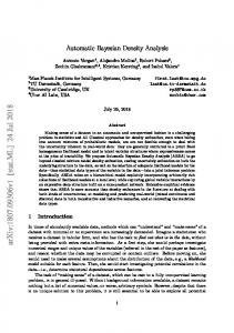
The “generalized travel-time misfit” ensures matching of the entire production history rather than single time point match and at the same time retaining most of the desirable properties of travel-time inversion. In “generalized travel time match” we seek an optimal time-shift at each well to minimize the production data misfit at the well. This is illustrated in Fig. 2.1c where the calculated water-cut response is systematically shifted in small time increments towards the observed response, and the data misfit is computed for each time increment. Taking well j as an example, the optimal shift will be given by the ∆t j that minimizes the misfit function, J pj =
n dj
∑ w [y (t i =1
ij
obs j
i
+ ∆t j ) − y
2
cal j
(t i )]
= f (∆t j )
…..…….(2.5)
Or, alternatively maximizes the coefficient of determination given by: ndj
R 2 (∆t j ) = 1 −
∑ [y i =1
obs j
(t i + ∆t j ) − y cal j (t i )
∑ [y ndj
i =1
obs j
(t i ) − y
obs j
]
2
]
2
…..…….(2.6)
16
~
Thus, the generalized travel-time at well j is the ‘optimal’ time-shift ∆ t j that 2 maximizes the R (∆tj ) or minimizes J pj as shown in Fig. 2.1d. It is important to point
out that the computation of the optimal time-shift does not require any additional flow simulations. It is carried out as a post-processing at each well after the calculated production response is derived using a flow simulation. The overall production data misfit can now be expressed in terms of a generalized travel-time misfit at all wells as follows J ∆ ~t =
nw
∑
j =1
(∆ ~t )
2
σ
…..…….(2.7)
j 2 j
Where, σ 2j is the error variance of the generalized travel time at well j by assuming C D a diagonal matrix. It is worth to mention here that using the data misfit in the objective function given by Eq. 2.3 as the generalized travel time reduces the computational burden during the minimization by reducing the data covariance matrix to be of order N w × N w and the data misfit vector to be of N w × 1 which are always of order of magnitude lower than the number of data points, N d . Thus, the concept of generalized travel time shift as the data misfit is well-suited for field-scale application and is used during this study. Accordingly, the objective function given by Eq. 2.3 using the generalized travel time as the data misfit, will be as follows: O(m ) =
[
]
1 ~ T −1 ~ T ∆ t C D ∆ t + (m − m prior ) C M−1 (m − m prior ) 2
……...……(2.8)
Where ∆~ t is the generalized travel time that minimizes the difference between the calculated and the observed data as given by Eq. 2.3. A detailed formulation of the generalized travel time shift under different scenarios will be studied in the next section. It is important to mention that the selection of the standard deviation of the data error is subjective and it depends upon the data itself. However a good guideline for selecting this parameter is given by Wu et al.5 and Wu36.
17
2.2.2 Generalized Travel Time Formulation In this section, a formulation of a general formula for the generalized travel time with respect to the travel time for two cases is given. The first case is when shifting the calculated response towards the observed and the second is when shifting the observed towards the calculated response.
Case1: Shifting calculated towards the observed Figs 2.2a, 2.2b show situations when the calculated is to the left of the observed and the calculated to the right of the observed, respectively. The general formula for the generalized travel time as function of the travel time at each point that satisfies the two situations in the next figures is as follows: ∆~ ti = t shift ,i − t cal ,i
i = 1,..nd
…..…….(2.9)
Where, for the first situation as shown in Fig. 2.2a, the sign of the generalized travel time is positive while for the other situation as shown in Fig. 2.2b, the sign is negative So, irrespective of the relative location of the calculated and the observed, Eq.2.9 satisfies the both situation for the case of shifting the calculated towards the observed. As we are shifting all the points with the same amount of shift, so the generalized travel time shift can be written as the average of all the shift for all the points as follows:
∆~ t =
1 nd
nd
∑ (t i =1
shift ,i
− t cal ,i )
……….(2.10)
In the vicinity of the solution or when the shape of the calculated response is close to that of the observed, t shift can be approximately equal to t obs as shown in Figs. 2.2a,b. Thus Eq.2.10 will be as follows:
∆~ t ≅
1 nd
nd
∑ (t i =1
obs ,i
− t cal ,i )
…...…..(2.11)
18
0.8
calculated
observed
0.6
~ ∆t L
shifted
~ ∆t r
0.4 0.3
~ ∆t 2
0.2 0.1 0
200
400
~ ∆t L
shifted
0.5
~ ∆t r
0.4 0.3
~ ∆t 2
0.2 0.1
~ ∆t 1
0
observed
0.6
0.5
~ ∆t 1
0
600
800
1000
0
1200
200
400
(a)
calculated
~ ∆t L
shifted
0.5
~ ∆t r
0.4
~ ∆t 2
0.2
calculated
0.6
1200
~ ∆t L
shifted
0.5
~ ∆t r
0.4 0.3
~ ∆t 2
0.2
~ ∆t 1
0.1
1000
~ ∆t
observed
0.7
water cut, fw
water cut, fw
0.8
~ ∆t
observed
0.3
800
(b)
0.8
0.6
600 time, days
time, days
0.7
~ ∆t
calculated
0.7
water cut, fw
water cut, fw
0.7
0.8
~ ∆t
~ ∆t 1
0.1
0
0 0
200
400
600 time, days
(c)
800
1000
1200
0
200
400
600
800
1000
1200
time, days
(d)
Fig. 2.2−Illustration for the formulation of generalized travel time shift, (a) Shifting the calculated towards the observed: calculated to the right of the observed, (b) Shifting the calculated towards the observed: calculated to the left of the observed, (c) Shifting the observed towards the calculated: calculated to the right of the observed, (d) Shifting the observed towards the calculated: calculated to the left of the observed
19
Case2: Shifting observed towards the calculated Figs 2.2c, 2.2d show situations when the calculated is to the left of the observed and the calculated to the right of the observed, respectively. The general formula for the generalized travel time as function of the travel time at each point that satisfies the two situations in the above figures is as follows: ∆~ ti = t shift ,i − t obs ,i
i = 1,..nd
…..…….(2.12)
Where, for the first situation as shown in Fig. 2.2c, the sign of the generalized travel time is positive while for the other situation as shown in Fig. 2.2d, the sign is negative. As we are shifting all the points with the same amount of shift, so the generalized travel time shift can be written as the average of all the shift for all the points as follows:
∆~ t =
1 nd
nd
∑ (t i =1
shift ,i
− t obs ,i )
……….(2.13)
In the vicinity of the solution or when the shape of the calculated response is close to that of the observed, t shift can be approximately equal to t cal as shown in Figs. 2.2c, d. Thus Eq.2.13 will be as follows:
1 ∆~ t ≅ nd
nd
∑t i =1
cal ,i
− t obs ,i
…...…..(2.14)
Notice here the difference in the formulation of the generalized time shift, Eqs. 2.11 and
2.14 for shifting the calculated towards the observed and the opposite. It should be mentioned that while using poor initial model, Eqs. 2.11 and 2.14 might not be good approximation. For example, situations might arise when there is observed water cut response and no calculated response and vise versa. Under such conditions, the generalized travel time shift is given by the difference between the breakthrough time
20
and the end of the observed response and vise versa. From our experience we have seen that during successive iterations the shape of the production response gets close to the observed and Eqs. 2.11 and 2.14 can be considered good approximate formulation for the generalized travel time misfit.
2.3 Prior Model The prior model parameter ( m ) used in this work is the permeability at each grid block which are modeled as correlated stationary Gaussian random fields with specified means ( m prior ) and covariance, C M . The prior covariance is an auto covariance between the permeability at each grid block and it is calculated by knowing the variogram model which consists of three main components; the variogram model, the sill and the range. For more than one type of model parameter, for example permeability and porosity at each grid block, the covariance matrix will be as follows: CK CM = C φ , K
C K ,φ C φ
…...……(2.15)
Where, C K is the covariance matrix of permeability derived from the permeability variogram modeling, Cφ is the covariance matrix of porosity obtained from the porosity variogram modeling, C K ,φ and Cφ , K are the cross covariance matrix between porosity and permeability and is obtained by modeling the cross variogram or by using the screening hypothesis of Xu et al.37 During this study, the model parameter is the permeability at each grid block which is assumed to have a log normal distribution. It should be mentioned here that the covariance matrix is a full matrix of order M x M (M is the number of model parameters, i.e. M is equivalent to the number of grid blocks). So for field-scale applications with large number of grid blocks, a certain form of parameterization38 or approximations using the “stencil” concept34,39 is required during inversion. The approximation using stencil will be discussed later in this chapter.
21
2.4 Optimization Algorithms The minimization of Eq. 2.8 or Eq. 2.3 requires an efficient minimization algorithm especially for large field-scale applications where, the number of model parameters is usually high of the order of thousands to million grid block permeabilities or porosities. There are two different methods of minimization algorithms for unconstrained objective function like that given in Eq. 2.8 or Eq. 2.3; the gradient-based algorithms15 such as the steepest descent, Newton, Gauss-Newton, Levenberg-Marquardt, conjugate gradient and Variable metric (sometimes called quasi-Newton) and the non-gradient based algorithm like simulated annealing, genetic algorithm, Monte Carlo methods, and neural networks. The non gradient-based algorithms are not practical compared to the gradient algorithms for large number of parameters and thus, the gradient-based algorithms are the one that are commonly used in reservoir inverse problems. The rates of convergence of each type of the gradient-based algorithms are different. The Newton type of search algorithms like Newton, Gauss-Newton, and LevenbergMarquardt have quadratic rate of convergence in the vicinity of the solution compared to the super-linear rate of convergence of the variable-metric algorithm and the linear rate of convergence of steepest descent and conjugate gradient.15 However, the advantage of steepest descent, conjugate gradient, and variable metric is that the computation of sensitivity matrix is not required. Instead, the only requirement is the gradient of the objective function which can be obtained using adjoint method and need only one forward run and a solution of the adjoint system of linear equation only once independent of the number of data or the number of wells.7,
26-29
Due to the rapid
convergence of the Newton type of search algorithms, the next sections will cover briefly the equations used during the minimization for Newton, Gauss-Newton, and Levenberg-Marquardt algorithms. 2.4.1 Newton Algorithm The Taylor series of the objective function O(m), given by Eq. 2.8, is as follows: 1 T O(m) = O(m 0 ) + [∇ m O(m 0 )] (m − m 0 ) + (m − m 0 ) T H 0 (m − m 0 ) + ..... 2
….(2.16)
22
Where, ∇ m O(m 0 ) is the gradient of the objective function with respect to the model parameter, m at m = m0 and H0 is the Hessian of the objective function at m = m0. Taking the gradient of Eq. 2.16, ∇ m O(m) = ∇ m O(m 0 ) + H 0 (m − m 0 ) + .....
……….(2.17)
Locating the point m at the optimum value of the O(m) is equivalent to locating the point where the gradient of O(m) vanishes. By setting ∇ m O(m) = 0 in Eq. 2.17, Eq. 2.16 becomes:
m = m 0 − H o−1∇ m O(m 0 )
…...…..(2.18)
Eq. 2.18 is the Newton algorithm and is written in general form as: m l +1 = m l − H l−1∇ m O(m l )
…………(2.19)
Where, (l) denotes the iteration level. Newton algorithm, Eq. 2.19, requires getting the Hessian and its inverse. For large scale problems, where number of model parameters is extremely high, the inverse of the Hessian matrix which is of order M x M is computationally difficult. In Variable metric method, the inverse of the Hessian in Eq. 2.19 is updated at each iteration. Zhang et al.7 used the variable metric method with the gradient of the objective function calculated using adjoint method and they used LBFGS15 to update the inverse of the Hessian starting with the covariance matrix as the initial guess. However, their method can be computationally efficient if the updated Hessian remains positive definite at each iteration which is not the case in general.
23
2.4.2 Gauss-Newton Algorithm By taking the gradient of the objective function given by Eq. 2.8, ~ ∇ m O(m l ) = GlT C D−1∆ tl + C M−1 (m l − m p )
……….(2.20)
Where, Gl is the sensitivity matrix of the generalized travel time with respect to the model parameter and it is given as: ~ ∂∆~ t1,l ∂∆ t1,l l ∂m2l ∂m~1 ∂∆~ t2 , l ∂∆ t2,l ~ T T l Gl = (∇ m (∆ tl ) ) = ∂m1 ∂m2l ~ ∂∆ tnw ,l ∂∆~ tnw , l l ∂m2l ∂m1
∂∆~ t1,l ∂m Ml ∂∆~ t 2 ,l ∂m Ml ∂∆~ tn w , l ∂m Ml n xM w
....…….(2.21)
By taking the gradient of Eq. 2.20,
(
)
~ ∇ m2 O(m l ) = H = (∇ m GlT ) ⋅ C D−1∆ tl + GlT C D−1Gl + C M−1
…...…..(2.22)
~ For small residual, ∆ tl , or for quasi-linear problems, the first term in Eq. 2.22 can be neglected, thus Eq. 2.22 becomes: H ≅ GlT C D−1Gl + C M−1
……….(2.23)
Substituting Eq. 2.20, and Eq. 2.23 in the Newton algorithm, Eq. 2.19,
[
m l +1 = m l − GlT C D−1Gl + C M−1
] [G −1
T l
~ C D−1∆ tl + C M−1 (m l − m p )
]
……….(2.24)
24
Eq. 2.24 is the Gauss-Newton formula used during the minimization. The difficulties of Eq. 2.24, is that updating the model parameter at each iteration requires obtaining the
[
inverse of the covariance matrix plus the inverse of the matrix GlT C D−1Gl + C M−1
]
both of
which are of order M x M. Tarantola34 and Chu et al.25 used a matrix inverse lemma to convert Eq. 2.24 in a form computationally efficient when the number of model parameters are greater than the number of data. This form is:
[
m l +1 = m p - C M G Tl C D + Gl C M GlT
] [∆~t − G (m −1
l
l
l
− mp )
]
….……(2.25)
The form given in Eq. 2.25 is called Modified Gauss-Newton, Appendix A shows the derivation of the Modified Gauss-Newton formula. Eq. 2.25 and Eq. 2.24 are mathematically equivalent, but the computation time for both is completely different.
[
]
Eq. 2.25 requires only the inverse of matrix C D + Gl CM GlT which is of order N w × N w ( N w is the number of wells) in using the generalized travel time as the data misfit. It is worth to mention here that starting an initial guess with poor model makes the residual too large and the approximation of the Hessian given by Eq. 2.23 will not be a valid assumption and this lead to a poor convergence of Gauss-Newton. Li40 shows that using Levenberg-Marquardt algorithm with high value of the damping factor at the initial iteration to damp the model changes can overcome the convergence problem of the high data misfit at the early iterations. Levenberg-Marquardt algorithm is discussed in the next section.
2.4.3 Levenberg-Marquardt Algorithm Bi41 modified Levenberg-Marquardt formula for application to the inverse problems to be in the following form: m
l +1
=m + l
mp − ml 1+α
[
- C M G Tl (1 + α ) ⋅ C D + Gl C M GlT
]
−1
1 ~ l ∆ tl − 1 + α Gl (m − m p )
.……(2.26)
25
α is the damping factor and for large α, the change in the model parameters per iteration is small. Li40 use high value of α equal to 104 or 105 at the initial iteration for large residual to ensure reduction in the objective function and whenever there is a reduction in the objective function from one iteration to the other, the value of α decreased by a factor of 10 until it becomes close to zero, where Eq. 2.26 tends to the original Modified Gauss-Newton, Eq. 2.25 which is a good assumption at small residual. The minimization algorithm given by Eq. 2.25 requires knowledge about the sensitivity matrix, G which is a very critical step during minimization. Chapter III will be devoted to show the calculation of the sensitivity matrix using the finite difference simulator as forward model. 2.5 Bayesian Formulation for Field-Scale Applications The central point for the second part of this chapter deals with reformulating the objective function, Eq. 2.8 resulting from the Bayesian approach and use the same approach of Gauss-Newton algorithm to reach to a system of equations for model updating in order to reduce the burden of matrix multiplications during the minimization process using the Modified Gauss-Newton, Eq. 2.25. Thus, reducing the computation time and making it well-suited for large-scale field applications. 2.5.1 Bayesian Formulation The objective function in the Bayesian formulation given by Eq. 2.8 is re-written in the following from:
1 O(m ) = e T e 2
……….(2.27)
Where, C − 12 ∆~t D l e= 1 − C 2 m l − m p M
(
)
...……..(2.28)
26
The minimization of the objective function given in Eq. 2.27 can be obtained by using Newton’s optimization algorithm given by Eq. 2.19 as follows: H δ m = −∇ m O(m)
……….(2.29)
Where, ∇ m O(m ) is obtained from Eq. 2.27 as follows:
[
∇ m O(m) = (∇ m e T ) e = GlT C D−1 / 2
]
C M−1 / 2 e
….……(2.30)
Letting the Jacobian, J, be as follows:
(
J = ∇ m eT
)
T
C −1 / 2 G = D −1 / 2 l CM
….……(2.31)
Substitute Eq. 2.31 in Eq. 2.30, ∇ m O(m) = J T e
...……..(2.32)
The Hessian is obtained by taking the gradient of Eq. 2.32 with respect to the model parameter (m):
(
H = ∇ m (∇ m O(m) ) = ∇ m (e T ∇ m e T T
= J T J + eT ∇ m J
) )=∇ T
m
e T (∇ m e T ) T + e T ∇ m (∇ m e T ) T
..….(2.33)
Similarly, as Gauss-Newton, by neglecting the second term of Eq. 2.33, Eq. 2.33 becomes:
H ≅ JTJ
……..(2.34)
27
The approximation for the Hessian, Eq. 2.34, is the same as that of the Gauss-Newton algorithm and is strictly valid near the solution (small misfit) or for quasilinear problems. Substituting Eqs. 2.32 and 2.34 in Eq. 2.29;
J T J δ m = −J T e
……….(2.35)
Eq. 2.35 is simply a least-squares solution to the following system of equations
J δ m = −e
….……(2.36)
Substitute Eqs. 2.28 and 2.31 in Eq. 2.36, − C − 12 ∆~t C − 12 G l D l δm = D 1 1 − C 2 m − m l C − 2 p M M
(
………(2.37)
)
Eq. 2.37 is mathematically equivalent to the Gauss-Newton formulation, Eq. 2.24 and in turn equivalent to the Modified Gauss-Newton formulation, Eq. 2.25. Appendix
A shows the mathematical equivalent between the two formulations, Eq. 2.37 and Eq. 2.24. Eq. 2.37 represents a system of linear equations and we use an iterative sparse matrix solver, LSQR42 for solving this system. LSQR is well suited for highly illconditioned systems and is widely used for large-scale tomographic problem in seismology.43 However, difficulties arise in the computation of the square root of the matrix inverse in Eq. 2.37. In practice, the data covariance matrix is assumed to be diagonal and is thus easy to manipulate. However, the covariance matrix for the model −1
parameters can be full and in general, the calculation of C M
2
will be computationally −1
prohibitive for large-scale inverse problems. Previous efforts to compute C M 2 analytically have been limited to exponential covariance model14. Vega44 proposes an
28
approach to approximate the square root of the inverse of the covariance using a numerical stencil which is general for any covariance models. The next section will give brief overview for approximating the square root of the inverse of the prior covariance matrix using the numerically derived “stencil”. The scaling of the computation time with respect to the model parameters for the conventional Bayesian formulation, Eq. 2.25, and Eq. 2.37 will be studied in terms of the number of multiplications required by each formulation after discussing the concept of the numerical stencil.
2.5.2 Square Root of the Inverse of the Covariance Using Numerically-Derived Stencil The exact analytical calculation of the square root of the inverse of the covariance can be done using the concept of matrix diagonalization.45 Since the covariance matrix is a symmetrical matrix so, its square root of the inverse can be calculated exactly using the following equation:
C M−1 / 2 = U T Λ−1 / 2 U
…….(2.38)
Where U is the matrix, whose columns are the eigenvectors of C M , Λ is the diagonal matrix whose diagonal elements are the eigenvalues of the covariance matrix C M . This computation is very difficult to handle especially for large field-scale cases where the covariance matrix is full and large. Another alternative is to use iterative algorithms like Newton method46 to get the square root of the inverse of the covariance matrix. However, this method requires the calculation of the inverse of the covariance per iteration, which makes it impractical for large-scale problems. Recent attempt used to approximate the square root of the inverse of the covariance matrix by obtaining analytically its stencil from the covariance kernel14 based on the previous works for calculating the inverse of the prior covariance matrix.34,39 However, the analytical approximation suffers from two major limitations; it is applicable only for the
29
exponential covariance and the ratio of the grid size to the range in the three directions need to be equal. Due to these limitations, Vega44 proposed a method that overcomes these limitations which based on two basic principles; First, the covariance matrix and the square root of its inverse can be constructed using their respective kernels, Second, the two kernels remain unchanged regardless of the size of the matrix. The following are the procedures used to approximate the square root of the inverse of the covariance matrix using a numerically-derived stencil. First, and the most important step, is choosing the size of the stencil, which depends mainly upon the ranges, the grid sizes and the number of gridblocks in the three directions. Selections of the stencil is a tradeoff between speed and accuracy and sensitivity study should be done to best select the stencil required depending upon the behavior of each problem. To make the method understandable, we assume that 5x5x5 stencil provide a good compromise between efficiency and accuracy, so a 5x5x5 stencil can be used to approximate the square root of the inverse of the covariance matrix. Second, the concept of matrix diagonalization, Eq.
2.38, is used to get the square root of the inverse of the covariance for 5x5x5 grid block (125x125 covariance matrix) by knowing the kernel of the covariance. This is equivalent to getting the kernel of the square root of the inverse of any covariance function in a discretized or numerical form other than obtaining the kernel analytically as before.14 Third, the set up of the 5x5x5 stencil is shown in Fig. 2.3. This stencil has only 27 distinct elements due to symmetry. Any column or any row of the covariance matrix calculated from the second step can be used to get the magnitude of each stencil presented in Fig. 2.3. Column 63 is selected for convenience, as it is the middle column to construct the magnitude of each stencil. Table 2.1 shows the location of the stencil in the 125 x 125 matrix constructed in the second step, which in turn gives the magnitude of each stencil. Finally, the approximation of the square root of the inverse of the covariance for the model under study is obtained by using the stencil constructed in Fig.
2.3 and its magnitude obtained from Table 2.1.
30
G(25) i-2, j-2, k-1
G(18) i-1, j-2, k-1
G(14) i, j-2, k-1
G(18) i+1, j-2, k-1
G(25) i+2, j-2, k-1
G(17) i-2, j-1, k-1
G(7) i-1, j-1, k-1
G(4) i, j-1, k-1
G(7) i+1, j-1, k-1
G(17) i+2, j-1, k-1
G(15) i-2, j, k-1
G(6) i-1, j, k-1
G(3) i, j, k-1
G(6) i+1, j, k-1
G(15) i+2, j, k-1
G(24) i+2, j+1, k -2
G(17) i-2, j+1, k-1
G(7) i-1, j+1, k-1
G(4) i, j+1, k-1
G(7) i+1, j+1, k-1
G(17) i+2, j+1, k-1
G(26) i+2, j+2, k -2
G(25) i-2, j+2, k-1
G(18) i-1, j+2, k-1
G(14) i, j+2, k-1
G(18) i+1, j+2, k-1
G(25) i+2, j+2, k-1
G(26) i-2, j-2, k-2
G(23) i-1, j-2, k-2
G(22) i, j-2, k-2
G(23) i+1, -j2, k-2
G(26) i+2, j-2, k-2
G(24) i-2, j-1, k-2
G(19) i-1, j-1, k-2
G(13) i, j-1, k-2
G(19) i+1, -j1, k-2
G(24) i+2, j-1, k-2
G(21) i-2, j, k-2
G(16) i-1, j, k-2
G(10) i, j, k-2
G(16) i+1, j, k-2
G(21) i+2, j, k-2
G(24) i-2, j+1, k-2
G(19) i-1, j+1, k-2
G(13) i, j+1, k-2
G(19) i+1, j+1, k -2
G(26) i-2, j+2, k-2
G(23) i-1, j+2, k-2
G(22) i, j+2, k-2
G(23) i+1, j+2, k -2
Layer K-2
Layer K-1
G(20) i-2, j-2, k
G(11) i-1, j-2, k
G(9) i, j-2, k
G(11) i+1, j-2, k
G(20) i+2, j-2, k
G(12) i-2, j-1, k
G(5) i-1, j-1, k
G(2) i, j-1, k
G(5) i+1, j-1, k
G(12) i+2, j-1, k
G(8) i-2, j, k
G(1) i-1, j, k
G(0) i, j, k
G(1) i+1, j, k
G(8) i+2, j, k
G(12) i, j+1, k
G(5) i-1, j+1, k
G(2) i, j+1, k
G(5) i+1, j+1, k
G(12) i+2, j+1, k
G(20) i-2, j+2, k
G(11) i-1, j+2, k
G(9) i, j+2, k
G(11) i+1, j+2, k
G(20) i+2, j+2, k
Layer K G(25) i-2, j-2, k+1
G(18) i-1, j-2, k+1
G(14) i, j-2, k+1
G(18) i+1, j-2, k+1
G(25) i+2, j-2, k+1
G(17) i-2, j-1, k11
G(7) i-1, j-1, k+1
G(4) i, j-1, k+1
G(7) i+1, j-1, k+1
G(17) i+2, j-1, k+1
G(15) i-2, j, k11
G(6) i-1, j, k+1
G(3) i, j, k+1
G(6) i+1, j, k+1
G(17) i-2, j+1, k+1
G(7) i-1, j+1, k+1
G(4) i, j+1, k+1
G(25) i-2, j+2, k11
G(18) i-1, j+2, k+1
G(14) i, j+2, k+1
Layer K+1
G(26) i-2, j-2, k+2
G(23) i-1, j-2, k+2
G(22) i, j-2, k+2
G(23) i+1, j-2, k+2
G(26) i+2, j-2, k+2
G(24) i-2, j-1, k+2
G(19) i-1, j-1, k+2
G(13) i, j-1, k+2
G(19) i+1, j-1, k+2
G(24) i+2, j-1, k+2
G(15) i+2, j, k+1
G(21) i-2, j, k+2
G(16) i-1, j, k+2
G(10) i, j, k+2
G(16) i+1, j, k+2
G(21) i+2, j, k+2
G(7) i+1, j+1, k+1
G(17) i+2, j+1, k+1
G(24) i-2, j+1, k+2
G(19) i-1, j+1, k+2
G(13) i, j+1, k+2
G(19) i+1, j+1, k+2
G(24) i+2, j+1, k+2
G(18) i+1, j+2, k+1
G(25) i+2, j+2, k+1
G(26) i-2, j+2, k+2
G(23) i-1, j+2, k+2
G(22) i, j+2, k+2
G(23) i+1, j+2, k+2
G(26) i+2, j+2, k+2
Layer K+2
Fig. 2.3−5x5x5 stencil used for the numerical approximation of the square root of the inverse of the covariance
31
Table 2.1–Location of the numerical stencil terms from column 63 of the square root of inverse of covariance of 5 × 5 × 5 grid Numerical Stencil Term
Row Number in Column 63
G(0) G(1) G(2) G(3) G(4) G(5) G(6) G(7) G(8) G(9) G(10) G(11) G(12) G(13) G14) G(15) G(16) G(17) G(18) G(19) G(20) G(21) G(22) G(23) G(24) G(25) G(26)
63 62 58 38 33 57 37 32 61 53 13 52 56 8 28 36 12 31 27 7 51 11 3 2 6 26 1
2.5.3 Computational Scaling Properties: Conventional vs Field-Scale Bayesian Formulation In comparing the computation effort required by each formulation, we assume that the computational effort is directly proportional to the number of multiplications required by each formulation and our objective is to show how the number of multiplications for each formulation behaves with increasing the number of model parameters. For this
32
purpose we will assume that the sensitivity matrix required by the both formulation is full and covariance matrix is full in case of the conventional Bayesian, while in case of the new Bayesian formulation, we will use the concept of the stencil discussed before to approximate the square root of the inverse of the covariance. Thus the matrix will be sparse and we will use the maximum number of the non zero values for each row to be equal to the Ns (i.e. Ns is the maximum number of stencil, which is equal to 125 in case of using 5x5x5 stencil).
Conventional Bayesian formulation The conventional Bayesian formulation is given by Eq. 2.25. The number of multiplication per iteration required is calculated as follows: -
multiplications -
Forming C M GlT :
-
Forming
C D + Gl C M GlT :
w
w
[
requires ( N w ⋅ M )
w
[C M ]M ×M ⋅ [G Tl ]M × N
[Gl ]N ×M ⋅ [C M G Tl ]M × N -
[Gl ]N ×M ⋅ [m l − m p ]M ×1
Gl (m l − m p ) :
Forming
It
(
)
requires N w ⋅ M 2 multiplications
w
requires
the
(
following
multiplication
)
, which require N w2 ⋅ M multiplications
] [∆~t − G (m − m )]: It require solving a system ~ ⋅ [g ] = [∆ t − G (m − m )] equations in the form of [C + G C G ] Forming C D + Gl C M GlT
−1
l
l
l
D
l
p
T l Nw×Nw
M
of
l
f
N w ×1
l
l
p
N w ×1
to get (gf). The LU Decomposition and LU back substitution is used to get (gf)
( )
and this operation requires45 N w3 multiplications. -
[
Forming C M GlT C D + Gl C M GlT
[C
M
G Tl
]
M ×Nw
[ ]
⋅ gf
N w ×1
] [∆~t − G (m −1
l
l
l
)]
−mp :
requires ( N w ⋅ M ) multiplications.
Adding up all the above operations, results in the total number of multiplications per iteration required by the conventional Bayesian approach. Z GN = N w M 2 + 2 N w M + N w2 M + N w3
…..…..(2.39)
33
Field-scale Bayesian formulation The field-scale Bayesian formulation is given by Eq. 2.37, by assuming that C D is diagonal matrix, thus Eq. 2.37 can be written as: ~ − ∆ tl Gl −1 δm = −1 C M 2 m p − m l C M 2
(
………(2.40)
)
We used LSQR42 as an iterative sparse matrix solver to solve the above augmented system of equations. I followed the exact algorithm given by Paige and Saunders42 in counting the number of multiplication required by solving Eq. 2.40, which can be written in the following form:
[A](N
w +M
)× M
[x]M ×1 = [b](N
w +M
……….(2.41)
)×1
The following is the number of multiplications required at each step in the algorithm: 1) Initializing: -
Forming [u1 ](N w + M )×1 = [b](N w + M )×1 :
[C ]
−1 / 2 M M ×M
[
⋅ mp − ml
]
M ×1
required
the
product
of
, which requires (M ⋅ N s ) multiplications, where Ns is
the maximum number of the stencil used to approximate the square root of the inverse of the covariance (i.e. maximum number of non zero values per each row of C M−1 / 2 ). -
Normalize [u1 ]( N w +M )×1 and get β1 : require (N w + M ) multiplications
-
Form
[v1 ]M ×1 = [AT ]M ×( N
the following form,
w +M )
[u1 ]( N
w +M
)×1
: It is equivalent to find the product in
[v1 ]M ×1 = [G T ]M ×N [u`1 ]N ×1 + [(C M−1 / 2 ) T ]M ×M [u1 ``]M ×1 , w
w
require (N w ⋅ M + M ⋅ N s ) multiplications -
Normalize [v1 ]M ×1 and get α1 : require (M ) multiplications
this
34
2) Start Iteration inside the LSQR loop for i=1,2,…..Niter, where Niter is the number of iteration 3) Bidiagonalization -
[u i +1 ]( N
Form
w +M
)×1
= [ A]( N w + M )×M [vi ]M ×1 − α i [u i ]( N w + M )×1 : require the following
two products; a- α i [u i ]( N w + M )×1 : require (N w + M ) multiplications b- [A]( N w + M )×M [vi ]M ×1 : is equivalent to forming the two products;
[G ]N ×M [vi ]M ×1 : require (N w ⋅ M ) multiplications w
[C ] [v ] −1 / 2 M M ×M
i M ×1
: require (N s ⋅ M ) multiplications
-
Normalize [u i +1 ]( N w + M )×1 and get βi+1 : require (N w + M ) multiplications
-
Form
[vi +1 ]M ×1 = [AT ]M ×( N
w +M
)
[ui +1 ]( N
w +M
)×1
− β i +1 [vi ]M ×1 : require the following
two products; a- β i +1 [vi ]M ×1 : require (M ) multiplications
[ ]
b- AT
M ×( N w + M )
[ ]
form, G T
[ui +1 ]( N
M ×Nw
w +M
)×1
: It is equivalent to find the product in the following
[u`i +1 ]N ×1 + [(C M−1 / 2 ) T ]M ×M [ui +1 ``]M ×1 , w
this require (N w ⋅ M + M ⋅ N s ) multiplications -
Normalize [vi +1 ]M ×1 and get αi+1 : require (M ) multiplications
4) Construct and apply next orthogonal transformation: in this step the number of multiplications is independent upon the number of gridblocks (M) or the number of wells (Nw), so its multiplications count is not considered as they are very trivial. 5) Update [x ]M ×1 , [w]M ×1 : -
Update [x ]M ×1 : require (M ) multiplications
-
Update [w]M ×1 : require (M ) multiplications
6) End of the iteration
35
Adding the number of multiplications mentioned at each step and inside the LSQR iteration loop, the total number of multiplications will be: Z Field scale Bayesian = 2( M ⋅ N s ) + ( N w ⋅ M ) + N w + 2 M +
N iter [2( N w ⋅ M ) + 2( M ⋅ N s ) + 2 N w + 6M ]
....…….(2.42)
Fig. 2.4 shows the behavior of each formulation with respect to the model size using Nw of 15 for the both formulation and using Ns and Niter for the field-scale Bayesian formulation to be 125, and 15 respectively. I assumed that the stencil used is 5x5x5, so the maximum value for Ns is 125.
1E+12
Conventional Bayesian 1E+11
Field Scale Bayesianl y = 15.34x1.998 R2 = 1
No. of Multiplications
1E+10
1E+09
1E+08
y = 4557.6x R2 = 1
10000000
1000000 100
1000
10000
100000
1000000
Grid Size
Fig. 2.4−Computational scaling for field-scale Bayesian vs conventional Bayesian
Clearly as shown from Eqs. 2.39 and 2.42 and from the figure above, the field-scale Bayesian formulation behaves linearly compared to the conventional Bayesian
36
formulation which behaves quadratically with respect to the model size. This shows that the new Bayesian formulation with the numerically calculated stencil is well suited for field-scale applications where the number of model parameters exceeds hundred thousands to millions. However, it is important to mention that the number of multiplications in the field-scale Bayesian formulation depend upon two additional parameters other than the conventional Bayesian. Those parameters are the inner iteration inside the LSQR loop, Niter and the number of stencil used, Ns. Selecting the stencil is the most important factor in choosing between the two formulations as for high Ns, the Field-scale Bayesian behaves close to the conventional Bayesian and due to the inner iterations inside the LSQR loop it might even behave worse than the conventional Bayesian formulation. That is why selecting the stencil used is the key in choosing which formula to use during the minimization. 2.6 Bayesian Approach as a Tool for Uncertainty Assessment The Bayesian approach gives very distinct advantage in associating probability distribution known as the posterior distribution with its estimate. Sampling the posterior distribution to generate a suite of realizations provides a good tool to assess the uncertainty in reservoir variables. Moreover, one can predict the uncertainty in the future performance of the reservoir by constructing statistics for the set of outcomes obtained from the realizations generated from the posterior distribution. Accordingly, the correct sampling of the posterior is a vital issue in accurately quantifying the uncertainties and many research works are devoted to find an efficient way for accurately sampling the posterior distribution. In general, there are two different types of sampling. The first type belongs to the methods that is known to sample rigorously, such as inversion, rejection, sequential realization, Gibbs sampler, Markov Chain Mont Carlo (MCMC), and Genetic algorithms.34
The second type belongs to those that are known to sample
approximately47,48
such as linearization about the maximum a posteriori estimate
(LMAP), randomized maximum likelihood (RML)49, and pilot point (PP) method.
37
The most common method used to sample the posterior distribution rigorously is the MCMC method and many of the approximate methods are just an approximation from the MCMC under some specific conditions. In this section, a brief introduction about the MCMC as a rigorous way of sampling and Randomized Maximum Likelihood (RML) as an approximate way of sampling is given for completeness. 2.6.1 Markov Chain Monte Carlo (MCMC) According to Cunha et al.50, a Markov chain is a sequence of random variables X(0), X(1),…X(n) where the probability distribution for X(n) is determined by the probability distribution of X(n-1). The set of all possible values for X(i) (i = 0,1,2,…n) is called the state space. The transition probability, Pijn gives the probability of obtaining state j at the nth location in the sequence if the random variable is in state i at the n-1 location in the sequence. Let us denote a particular realization of a certain reservoir properties by mi, with the probability associated with it to be πi, where π is the posterior probability distribution that we want to sample from and πi is the probability of sampling mi from the posterior (i.e. π(mi)). The objective is to generate a new realization or new state mj with the probability associated with it to be πj such that the transition probability, Pij of obtaining the state mj from state mi satisfies the following conditions51, 1- It is possible to get from any one state to another in a finite number of transitions, 2- π j = ∑ π i Pij
………(2.43)
i
Thus, the Markov chain will be stationary and ergodic (independent on initial conditions) and π will be the stationary distribution, which is the posterior distribution that we want to sample from. In Metropolis-Hasting algorithm, the transition probability, Pij is partitioned into two parts: Pij = α ij qij , where qij is the probability of proposing transition from state mi to state mj and αij is the probability of accepting the proposed transition mj as the next state in the Markov chain and it is given by:
38
π j q ji π i qij
α ij = min 1,
……….(2.44)
Two important points should be taken into consideration in sampling the posterior distribution using MCMC. The first is selection of qij (i.e. the PDF used to sample for the new state, mj). If qij is close to the posterior distribution that we want to sample from, most of the transitions will be accepted and the chain converges quickly to the posterior distribution. The second point is the way of sampling, for example, whether the twopoint swapping, where two model parameter in two different grid blocks are swapped per each transition to the new state or the local perturbation, where one model parameter is perturbed per transition, or the global perturbation, where all the model parameters are perturbed once per transition. Oliver et al.51 shows that local perturbation is more efficient in generating independent realizations in the Markov chain for highly nonlinear problem, while global perturbation is efficient in linear to slightly non linear problems. 2.6.2 Randomized Maximum Likelihood (RML) Oliver et al.49 propose a two step transition to a new state in MCMC that has a high probability of acceptance in the Metropolis-Hasting algorithm. The first step is to propose an unconditional realization from the prior probability distribution using any unconditional simulation technique, like sequential Gaussian simulation.52 The second step involves the history matching of the unconditional model to the production data that has noise added. The conditional model resulting from the history matching process will be a new state in the Markov chain. Because the acceptance rate was found very high (approximately 95% for a small highly non-linear problem), they suggested to accept all the new state proposed in the chain. In this study, we applied this method to generate realizations and assessing the uncertainty. The following is the algorithm for generating realizations from RML method:
39
1. Generate an unconditional realization of the reservoir model parameters,
[
]
mu ← N m p , C M , by assuming that the variogram of the prior model is known, this can be done by using sequential Gaussian simulation or any unconditional simulation technique 2. Generate a realization of the data, d u ← N [d obs , C D ] , by adding a random noise to the observed data 3. Compute the set of model variables, m , that minimizes the function: O(m ) =
1 (m − mu )T C M−1 (m − mu ) + 1 [g (m ) − d u ]T C D−1 [g (m ) − d u ] 2 2
………(2.45)
2.7 Chapter Summary Bayes theory provides a good statistical tool to integrate static with dynamic data and assess the uncertainty associated with the estimate. This chapter consists of three major parts. The first part gives a brief introduction about Bayes theory and shows the three important components for automatic history matching in Bayesian framework. Those components are the data misfit, the prior term, and the optimization algorithm. For the data misfit, the general three types of the data misfit are explained, with special reference to the one that is used during this study which is the “Generalized Travel Time Misfit”. For the prior term, a brief introduction is given about the covariance matrix calculation in case of single type of model parameter, like permeability and different type of model parameters, for example permeability and porosity. For the optimization algorithm, a brief introduction about gradient-based and gradient-free algorithms with detailed overview about the gradient based algorithms especially; the Newton type algorithms are given. The second part of this chapter concerns with the new Bayesian formulation that is well-suited for field-scale applications. A numerical approximation of the square root of the inverse of the covariance using the stencil is required by the new formulation and is discussed. Finally the computational scaling in the form of the number of multiplication required by both the conventional and the field-scale Bayesian is investigated. From the
40
computational scaling it was found that the field-scale Bayesian scales linearly with the increase in the number of model parameters compared to the conventional Bayesian which scales quadratically. This makes the field-scale Bayesian well suited for fieldscale applications from the computational point of view. The last part of this chapter gives one of the most important applications of the Bayes theory which is the uncertainty assessment. In this part a brief introduction about different types of sampling from the posterior distribution for uncertainty assessment are given with a special reference to the rigorous one, which is the MCMC and the approximate one which is used during this study, the Randomized Maximum Likelihood (RML) method.
41
CHAPTER III SENSITIVITY COMPUTATION USING FINITE DIFFERENCE MODELS Sensitivity computation is a very critical step in automatic history matching process when using gradient-based optimization algorithm like Gauss-Newton or LevenbergMarquardt to minimize the objective function given in the previous chapter. The sensitivity is defined as the change in the production response due to a small change in the model parameter. Chapter I discusses in details the different methods for sensitivity computation using finite difference as the forward model. In this chapter, we present the computation of the generalized travel time sensitivity with respect to the model parameter using the adjoint method (optimal control theory) and the streamline-based sensitivity for finite difference models. A complete detail for developing the generalized travel time sensitivity using adjoint method for 3D, two phase flow is given with a brief introduction for the generalized travel time sensitivity computation from streamlinebased sensitivity. 3.1 Adjoint Method-Based Sensitivity There are three different approaches presented in the literature for sensitivity formulation using the adjoint method. The first approach shows the sensitivity formulation starting from a complete continuous form of the flow equation26,27, the second approach shows the formulation starting from a semi-continuous form of the flow equation28,8, where only the left hand side of the flow equation is discretized leaving the right hand side in a continuous form. The third approach shows the formulation in a complete discretized form,5-7,29 where the flow equation is completely discretized. In this work, we will apply the third approach to develop the formulation of the generalized travel time sensitivity for 3D two phase flow problems. The sensitivity computation using the adjoint method requires the following three steps; the forward model formulation, adjoint system formulation, and finally the
42
sensitivity coefficient formulation. The next sections will describe these steps in more details. 3.1.1 Forward Model Formulation In our work the forward model is IMPES finite difference simulator that is developed to handle 3D, two-phase, oil-water problems. Then later, we used a commercial simulator (viz. ECLIPSE53) for modeling fluid flow in porous media and the adjoint method-based sensitivity calculation for practical applications. The equations governing the two-phase flow equation in the reservoir after neglecting capillary pressure are as follows: Oil: K ∂ φ So C1 ∇ • ro [K ] (∇p ( x, y, z , t ) − γ o ∇D( x, y, z ) ) − qˆ o ( x, y , z , t ) = ∂t C 2 Bo µ o Bo
…..(3.1)
Water: K rw [K ] (∇p( x, y, z, t ) − γ w ∇D( x, y, z ) ) − qˆ w ( x, y, z, t ) = ∂ φ S w ..…(3.2) C1 ∇ • ∂t C 2 Bw µ w Bw
S o + S w = 1.0
……..…(3.3)
Where, C1 equal 1.127x10⁻³, C 2 equal 5.615, Bm is the formation volume factor in bbl/STB for m stands for o (oil), w (water), K rm is the relative permeability for phase m , µ m is the viscosity for phase m in cp, [ K ] is the permeability tensor, K x 0 0
0 Ky 0
0 0 K x , K y , K z are the permeability in md, p is the pressure at x,y,z K z
43
location and at time t, φ is porosity, qˆ ( x, y, z , t ) is the source or the sink term per unit
bulk volume, STB/ft3-day it is zero at all the locations except at the location of the wells. It is positive for production wells and negative for injection wells, S m is the phase m saturation, γ m is the specific weight of oil and water, and its unit is in psi/ft, and D is the depth at x,y,z location. By multiplying Eqs. 3.1 and 3.2 by bulk volume, Vb , of each grid block and using finite difference to discretize Eqs. 3.1 and 3.2, and neglecting the formation compressibility, the following discretized equations are formed: Oil:
Tox ,i +1 / 2, j ,k ( pi +1, j ,k − pi , j ,k − γ oi +1 2, j , k ( Di +1, j , k − Di , j ,k )) − Tox ,i −1 / 2, j ,k ( pi , j ,k − pi −1, j , k − γ oi −1 2, j , k ( Di , j ,k − Di −1, j , k )) + Toy ,i , j +1 / 2, k ( pi , j +1,k − pi , j ,k − γ oi , j +1 2,k ( Di , j +1,k − Di , j ,k )) − Toy ,i , j −1 / 2,k ( pi , j ,k − pi , j −1,k − γ oi , j −1 2,k ( Di , j ,k − Di , j −1,k ))
…….…..(3.4)
+ Toz ,i , j ,k +1 / 2 ( pi , j ,k +1 − pi , j ,k − γ oi , j ,k +1 2 ( Di , j ,k +1 − Di , j ,k )) − Toz ,i , j ,k −1 / 2 ( pi , j ,k − pi , j ,k −1 − γ oi , j ,k −1 2 ( Di , j ,k − Di , j ,k −1 )) − q o ,i , j ,k =
Vb φi , j ,k C 2 ∆t
l
[(S
bo )i , j ,k − (S o bo )i , j ,k l +1
o
l
]
Water:
Twx ,i +1 / 2, j , k ( p i +1, j , k − pi , j , k − γ wi +1 2, j ,k ( Di +1, j ,k − Di , j ,k )) − Twxl ,i −1 / 2, j ,k ( p i , j ,k − pi −1, j ,k − γ wi −1 2, j ,k ( Di , j ,k − Di −1, j ,k )) + Twy ,i , j +1 / 2,k ( pi , j +1,k − pi , j ,k − γ wi , j +1 2,k ( Di , j +1,k − Di , j ,k )) − Twy ,i , j −1 / 2,k ( pi , j ,k − pi , j −1,k − γ wi , j −1 2,k ( Di , j ,k − Di , j −1,k )) + Twz ,i , j ,k +1 / 2 ( pi , j ,k +1 − pi , j ,k − γ wi , j ,k +1 2 ( Di , j ,k +1 − Di , j ,k )) − Twz ,i , j ,k −1 / 2 ( pi , j ,k − pi , j ,k −1 − γ wi , j ,k −1 2 ( Di , j ,k − Di , j ,k −1 )) − q w,i , j ,k =
Vb φi , j ,k C 2 ∆t
l
[(S
bw )i , j ,k − (S w bw )i , j ,k l +1
w
l
]
……..…(3.5)
44
Where, q m is the phase m rate in STB/day, Tm is the phase m transmissibility in x, y, and z directions, bm is the reciprocal of the formation volume factor of phase m , ∆t is the time step, and i = 1,2,……nx, j = 1,2,….ny, k = 1,2,….,nz. Eqs. 3.4, 3.5 with Eq. 3.3 are solved to calculate the pressure and water saturation at
each grid block per each time step, in addition to the production history at each well. Since we are interested in matching only the water cut from the wells, so the production history reported is only the water cut at each well. Also, the pressure and water saturation at each grid block per each time step should be stored, as it will be used during sensitivity computation. 3.1.2 Adjoint System Formulation
In formulating the adjoint system of equations, the discretized flow equations, Eqs. 3.4 and 3.5 are given in the following form:
[
Fml +1 ( p l +1 , S wl +1 , K x , K y , K z ) = Vφl,+i ,1j , k (bm S m )i , j , k − (bm S m )i , j , k l +1
l
]
………….(3.6)
It is important to note that Eq. 3.6 gives the difference equations in fully implicit form, thus it is important that the simulator used to be in fully implicit form for consistency and for the pressure and water saturation calculated from the simulator to satisfy Eq. 3.6, which is used during our formulation of the adjoint system of equations as our forward model. Throughout, l refers to time step index; 0, 1, 2,…… L − 1 , where L is the total time step index used in the forward model.
Vφl,+i ,1j ,k =
Vb φi , j ,k C 2 ∆t l
=
∆xi ∆y j ∆z k φi , j ,k C 2 ∆t l
…………..(3.7)
From this point on, we will assume that there are M simulator grid blocks that is ordered from 1,2,3,…,M and then
45
Vφl,+i ,1j ,k will be written as, Vφl +1
Vφl,+11 0 0 l +1 0 Vφ , 2 = 0 0 Vφl,+31 0 0 0
0 l +1 Vφ , M M ×M
[
Pressure will be written in the vector form as: p l = p1l
[
Saturation will be also written as: S ml = S ml 1
S ml 2
p 2l
l S mM
…….…..(3.8)
p Ml
]
T
.………(3.9)
]
T
.…...…(3.10)
The reciprocal of the formation factor is also written in the vector form as:
[
bml = bml 1 bml 2
l bmM
]
T
...……..(3.11)
[
The rate also can be written as: q ml = q ml 1
q ml 2
l q mM
]
T
..……...(3.12)
However, q m vector is sparse as small numbers of grids, which are the well grid blocks are only have non zero q m Similarly porosity, φ , permeability, K x , K y , K z will be written in the vector as shown in Eqs. 3.9 – 3.12. Accordingly, Eq. 3.6 can be written in the following form:
Fml +1 ( P l +1 , S wl +1 , K x , K y , K z ) = Aml +1 − Aml
...…….(3.13)
Where,
Aml +1 ( P l +1 , S wl +1 , φ ) = Vφl +1 (bm S m ) Aml ( P l , S wl , φ ) = Vφl +1 (bm S m )
l
l +1
…...…..(3.14)
....…..…(3.15)
46
Fm is independent of porosity and depends on permeability, while Aml +1 and Aml are porosity-dependent and permeability-independent. Accordingly the following equations hold:
[
]
[
]
∇ φ ( Fml +1 ) T = Ο
……….(3.16)
[
]
[
]
……….(3.17)
∇ K x ( Aml ) T = ∇ K y ( Aml ) T = ∇ K z ( Aml ) T = Ο
...……..(3.18)
∇ K x ( Aml +1 ) T = ∇ K y ( Aml +1 ) T = ∇ K z ( Aml +1 ) T = Ο
[
]
[
]
[
]
Ο in Eqs. 3.16 -3.18 is a null M x M matrix.
Our objective is to get the sensitivity of the generalized travel time shift, ∆~ t , at each well, let us denoted now by g ( p 1 ,....., p l , S w1 ,......., S wl , K x , K y , K z , φ ) subject to the set of constraint equations in the form of finite difference equations given by Eq. 3.13 at each grid block for each time step. In other words, we want to see how the perturbation in Kx, Ky, Kz, and φ at each grid block will affect the generalized travel time at each well. So, a two M–dimensional vectors of Lagrange multipliers are used to adjoin g with the finite difference equations to form the augmented objective function J , where M is the number of grid blocks, as follows:
λlo = [λlo1 λlo 2
λloM ]
λlw = [λlw1 λlw 2
λlwM ]
T
...…….(3.19)
T
….....….(3.20)
Thus the equation after adjoining the g function with the constraint equations will be:
47
J =g+
L −1
∑ ∑ (λ
m =o , w l =0
l +1 T m
[
) Fml +1 − Aml +1 + Aml
]
..……..(3.21)
From Eq. 3.21 and Eq. 3.13, it is clear that J and g are equivalent. Thus, the partial derivative of J with respect to the model parameter is equivalent to the partial derivative of g . The g function in our case is the generalized travel time shift for each well at the well location, but to keep the formulation general the adjoint equation will be formulated for any arbitrary function g, which is at certain location in reservoir. By taking the total differentiation of Eq. 3.21 with respect to the state variables, pressure and water saturation and with respect to the control variables, K x , K y , K z , and φ .
L −1
dJ = dg +
∑ ∑ (λ
m = o , w l =1
( [
) ∇ p l Fml − Aml
l T m
] ) dp T T
( [ ]) ( [ ])
l
( [
+ ∇ S l Fml − Aml w
] ) dS T T
l w
( [ ]) ( [ ]) ( [ ]) ( [ ]) ( [ ])
T T T T T l +1 T dK x + ∇ k y Fml +1 dK y + ∇ k z Fml +1 dK z − l +1 T ∇ k x Fm L −1 (λ m ) T T T T + ∑ ∑ l +1 T l T l T l l T l dφ + ∇ φ Am dφ + ∇ p l Am dp + ∇ S l Am dS w ∇ φ Am m =o , w l =0 w L + BT ………..(3.22)
Where, BTL is calculated from the following equation:
BT L =
( [
(λ mL ) T ∇ p L FmL − AmL m =o, w
∑
]
) dp + (∇ [F
T T
L
S wL
L m
− AmL
]
) dS
T T
L w
……….(3.23)
Since initially P, Sw are always known and the variation in the control variables m ( K x , K y , K z , and φ ) will not have any effect on the initial pressure and water
saturation at each grid block, thus,
48
dp 0 = dS w0 = 0
……..…(3.24)
Thus, any term multiplied by dp 0 and dS w0 had to be neglected from Eq. 3.22. Similarly, by taking the total differentiation of g as it is also depend on state and control variables, thus the total differentiation of g will be:
([
[
]
]
) [
[
]
]
[
]
[
]
L −1 T T T T T T dg = ∑ ∇ p l g dp l + ∇ S l g dS wl + ∇ K x g dK x + ∇ K y g dK y + ∇ K z g dK z + ∇ φ g dφ w l =1
...……..(3.25) Substituting Eq. 3.25 in Eq. 3.22,
( )
(∇ [F
( )
(∇ [F
l ∑ λ m L −1 m = o , w dJ = ∑ l =1 l ∑ λ m m =o , w L −1 l +1 ∑ ∑ λ m m = o , w l =0
( )
L −1 l +1 ∑ ∑ λ m m = o , w l =0
T
( )
T
T
T
p
S wl
l m
l m
− Aml
] ) + (∇ g )
− Aml
] ) + (∇ g )
T T
Kx
T l +1 T m
(∇ [F ] ) + (∇ Kz
T l +1 T m
T
(∇ [F ] ) + (∇
p
l
T T
+ ∑ λlm+1 m =o,w
T
+ ∑ λlm+1 m =o,w
p
S wl
T
L −1 T g dK + ∑ ∑ λlm+1 Kx x m =o , w l =0
)
Kz
T T
φ
l
+ + T l dS w
T l T m
l
(∇ [A ] )
( )
T
(∇ [A ] ) dp
( )
S wl
( )
T
l T m
(∇ [F ] ) + (∇ g ) dK Ky
T l +1 T m
T
Ky
T g dK z +
)
( [ ] ) − (∇ [A ] ) + (∇ g ) dφ + BT
L −1 l l +1 T ∑ ∑ λ m ∇ φ Am m = o , w l =0
( )
l
T l +1 T m
T
φ
L
….……(3.26) Eq. 3.26 is very important to understand it physically. It shows how the change in
the control variables m ( K x , K y , K z , and φ ) at each grid block affect the pressure and water saturation at each time step in each grid block. This in turn affect the augmented objective function (J) which is equivalent to the change in g (generalized travel time at each well) as seen from Eq. 3.21.
y
+
49
Since, the objective is to get the sensitivity of (g) with respect to the control variables, which are the permeability and porosity, thus to remove the dependency of J from pressure and water saturation, we choose the adjoint variables to insure that the coefficients of dp l and dS wl in Eq. 3.26 vanish. This will get the following adjoint system of equations.
∑
[(∇
∑
[(∇
m =o,w
m =o,w
pl
[F
S wl
l m
[F
l m
− Aml
] )λ
− Aml
T
l m
] )λ T
l m
]
[ ]
T
+ ∇ p l Aml λlm+1 = −∇ p l g
[ ]
T
]
+ ∇ S l Aml λlm+1 = −∇ S l g w
……….(3.27)
....…….(3.28)
w
Also, to remove the dependency of the change of pressure and water saturation at the end of simulation, dp L and dS wL due to the change of the control variables, we set
λ Lw = λoL = 0
…….…(3.29)
This will be the initial condition to solve the adjoint system of equation, Eqs. 3.27 and 3.28 backward in time, to get the Lagrange multipliers, λ m at each grid block per each
time step. The right hand side of Eq. 3.29 is M-dimensional column vector of zero values. Thus, from Eq. 3.23 and Eq. 3.29,
BT L = 0
……….(3.30)
From Eqs. 3.27, 3.28, and 3.30, the change in the augmented function J in Eq. 3.26, will be:
50
L −1 dJ = ∑ ∑ λlm+1 m =o , w l =0
( )
T
L −1 l +1 ∑ ∑ λ m m = o , w l =0
( )
L −1 l +1 ∑ ∑ λ m m =o , w l =0
Kx
T
( )
T
(∇ [F ] ) + (∇ T l +1 T m
Kx
T g dK x +
)
(∇ [F ] ) + (∇ g ) dK Ky
T l +1 T m
T
Ky
(∇ [F ] ) + (∇ Kz
T l +1 T m
y
+
……….(3.31)
T g dK z +
)
( [ ] ) − (∇ [A ] ) + (∇ g ) dφ
L −1 l l +1 T ∑ ∑ λ m ∇ φ Am m =o , w l =0
( )
Kz
T T
φ
T l +1 T m
T
φ
In our work, the (g) function is the generalized travel time shift at the well j , and according to the formulation given in the previous chapter assuming we are shifting the calculated towards the observed; the generalized travel time shift at well j is given by:
1 ~ g = ∆t j ≅ n dj
ndj
∑ (t i =1
i obs , j
i − t cal ,j
)
..……..(3.32)
Where, ndj are the number of data points for well j , (i) is the index for the data point at time t i . The gradient of the scalar function g in the adjoint system of equations, Eqs. 3.27 and 3.28 are given by taking the gradient of Eq. 3.32 as follows:
~ ∂∆ t j ~ ∇ pl g = ∇ Pl ∆ t j = l ∂P1
∂∆~ tj
~ ∂∆ t j ~ ∇ Sl g = ∇ Sl ∆t j = l w w ∂S w1
∂∆~ tj
∂P2l
∂S wl 2
T ∂∆~ tj ∂PMl
T ∂∆~ tj l ∂S wM
……….(3.33)
….……(3.34)
It should be noted that Eqs. 3.33 and 3.34 are vectors of non zero elements at grid blocks containing producing wells only. At grid blocks of producing wells, the partial
51
derivatives of the generalized travel time with respect to pressure and water saturation are given as follows: tj ∂∆~
i n 1 1 ∂t cal , j ∂ dj i i ) t ≅ − − ⋅ l ∑ (t obs ,j cal , j ndj ∂P i =1 ndj ∂p l
...…….(3.35)
i n ∂ dj i 1 1 ∂t cal , j i ≅ ⋅ ∑ t obs , j − t cal , j ≅ − ndj ∂S wl i =1 ndj ∂S wl
.………..(3.36)
≅
∂P l ∂∆~ tj ∂S wl
(
)
Where at time step index, l , that is corresponding to the same observed time, t i , the derivatives of Eqs. 3.35 and 3.36 exist, otherwise, the derivative will vanish. So, strictly speaking in solving the adjoint system of equations backward in time the vectors of the source term or the right hand side of the adjoint system of equations will be null vectors except at the time corresponding to observed data point time, where the non zero elements in those vectors will be corresponding to the grid blocks containing producing wells only. The derivatives in the right hand side of Eqs. 3.35 and 3.36 are given as follows: i i i 1 ∂t cal , j 1 ∂t cal , j ∂K ∂f wcal , j − =− ⋅ ⋅ i ⋅ ndj ∂K ∂f wcal ndj ∂p l ∂p l ,j
……….(3.37)
The change in permeability has opposite effect with respect to travel time and water cut; the increase in permeability leads to a decrease in travel time and increase in water cut, thus: i ∂t cal ,j
∂K
⋅
∂K 1 1 =− i =− l i i l −1 l l −1 ∂f wcal , j ∂f wcal , j ∂t cal , j ( f wcal , j − f wcal , j ) (t cal , j − t cal , j )
…..….(3.37a)
52
Substituting Eq. 3.37a in Eq. 3.37 i i ∂f wcal 1 ∂t cal , j 1 1 ,j − = ⋅ l ⋅ l l −1 l l −1 l ndj ( f wcal , j − f wcal , j ) (t cal , j − t cal , j ) ∂p ndj ∂p
.....…..(3.37b)
Similarly, the derivative with respect to water saturation is as follows:
−
i i ∂f wcal 1 ∂t cal , j 1 1 ,j = ⋅ ⋅ l l l l −1 l l −1 ndj ∂S w ndj ( f wcal , j − f wcal , j ) (t cal , j − t cal , j ) ∂S w
……….(3.38)
Where, l in Eqs. 3.37b and 3.38 is corresponding to time, t i at the observed point (i) as mentioned before, while l − 1 is corresponding to time t l −1 which is ( t i − ∆t ), where ∆t is the time step used in the simulation. This is a backward finite difference approximation to get numerically the derivative of water cut with respect to time at time t i assuming small ∆t used during simulation. It is important to mention that in general t i − ∆t is not equal to t i −1 , which is the time for the next observed data point. The partial derivative of water cut with respect to pressure and water saturation is obtained as follows:
i ∂f wcal ,j
∂p l
i K K rw ⋅ WI k , j ⋅ Pji,k − Pwfi , j ∑ l B µ k =1 w w k , j ∂ = l i K ∂p K K rw K roi i i i i ∑ ⋅ ⋅ − + WI P P ∑ i i ⋅ WI k , j ⋅ Pj ,k − Pwf , j k, j j ,k wf , j k =1 µ wi Bwi k , j B µ k =1 o o k , j
(
(
)
)
(
)
………..(3.39)
53
i ∂f wcal ,j
∂S wl
i K K rw ⋅ WI k , j ⋅ Pjl,k − Pwfl , j ∑ l k =1 µ w B w k , j ∂ = l i K ∂S w K K rw K roi i i ∑ ⋅ WI k , j ⋅ Pj ,k − Pwf , j + ∑ i i ⋅ WI k , j ⋅ Pji,k − Pwfi , j i i k =1 µ w Bw k , j k =1 µ o Bo k , j
(
(
)
)
(
)
……….(3.40) Where, K is the total number of layers opened for production for well (j), WIk,j is the well index for layer k at well j, which is independent of pressure and water saturation, i , K roi are the relative permeability to water and oil at the grid block of well (j) and at K rw
the observed point (i) corresponding to time t i . Bwi , Boi are the water and oil formation volume factors at well j grid block and at the observed point (i) corresponding to time t i . µ wi , µ oi are the water and oil viscosity at well j grid block and at the observed time t i . Pji,k is the pressure at the well j grid block and at time t i . Pwfi , j is the bottom hole
pressure at well j grid block and at time t i and it is assumed constant through the whole perforation intervals by neglecting the friction loss of the tubing across the perforation intervals. Appendix B shows a detailed derivative of Eqs. 3.39 and 3.40 with respect to pressure and water saturation at each individual grid block opened for production. It is important to mention that at each time step the adjoint system of equations, Eqs. 3.27 and 3.28 are solved only nw times with the same matrix but with different right
hand side. While in case of the conventional amplitude inversion the adjoint systems have to be solved nd (number of data points) times. This reduces the computational difficulties especially in large field-scale problems. 3.1.2.1 Adjoint System Formulation in i,j,k Notation
Till this point the adjoint system of equations are obtained in the form of M simulator grid blocks arranged from 1,2,3,.. M. The objective of this section to obtain the adjoint system of equations given by Eqs. 3.27 and 3.28 in a conventional form of i,j,k notation.
54
We will show the procedures for changing Eq. 3.27 into the i,j,k notation and similarly the same procedures will be for Eq. 3.28. Eq. 3.27 can be written in the following form:
[ ] λ − ∇ [q ] λ − ∇ [A ] λ + ∇ [ f ] λ − ∇ [q ] λ − ∇ [A ] λ + ∇ [A ] λ + ∇ [A ] λ = −∇ g
∇ p l f ol p
l
T
l o
l T w
l T o
pl
l w
p
l
l o
l T o
pl
l +1 o
l T o
p
l
l o
l T w
pl
l +1 w
l T w
l w
p
pl
l T w
l w
....……(3.41)
l
Where, from Eqs. 3.4, 3.5, 3.6, and 3.7, f ol , f wl are given as follows: f ol,i , j ,k = Toxl ,i +1 / 2, j ,k ( pil+1, j ,k − pil, j ,k − γ oil +1 2, j ,k ( Di +1, j ,k − Di , j ,k )) − Toxl ,i −1 / 2, j ,k ( pil, j ,k − pil−1, j ,k − γ oil −1 2, j ,k ( Di , j ,k − Di −1, j ,k )) + Toyl ,i , j +1 / 2,k ( pil, j +1,k − pil, j ,k − γ oil , j +1 2,k ( Di , j +1,k − Di , j ,k )) − Toyl ,i , j −1 / 2,k ( pil, j ,k − pil, j −1,k − γ oil , j −1 2,k ( Di , j ,k − Di , j −1,k ))
.......…..(3.42)
+ Tozl ,i , j ,k +1 / 2 ( pil, j ,k +1 − pil, j ,k − γ oil , j ,k +1 2 ( Di , j ,k +1 − Di , j ,k )) − Tozl ,i , j ,k −1 / 2 ( pil, j ,k − pil, j ,k −1 − γ oil , j ,k −1 2 ( Di , j ,k − Di , j ,k −1 )) l f wl ,i , j ,k = Twxl ,i +1 / 2, j ,k ( p il+1, j ,k − pil, j ,k − γ wi +1 2 , j , k ( Di +1, j , k − Di , j , k )) l − Twxl ,i −1 / 2, j ,k ( pil, j ,k − pil−1, j ,k − γ wi −1 2 , j , k ( Di , j , k − Di −1, j , k ))
+ Twyl ,i , j +1 / 2,k ( pil, j +1,k − pil, j ,k − γ wil , j +1 2,k ( Di , j +1,k − Di , j ,k )) l − Twyl ,i , j −1 / 2,k ( p il, j ,k − pil, j −1,k − γ wi , j −1 2 , k ( Di , j , k − Di , j −1, k ))
+ Twzl ,i , j ,k +1 / 2 ( pil, j ,k +1 − pil, j ,k − γ wil , j ,k +1 2 ( Di , j ,k +1 − Di , j ,k )) − Twzl ,i , j ,k −1 / 2 ( pil, j ,k − pil, j ,k −1 − γ wil , j ,k −1 2 ( Di , j ,k − Di , j ,k −1 )) The first term in Eq. 3.41 is given in matrix form as follows:
….……(3.43)
55
[ ]
∇ p l f ol
T
∂f ol,1 l ∂p1 ∂f ol,1 l = ∂p 2 l ∂f o ,1 ∂p l M
∂f ol, M ∂p1l ∂f ol, M ∂p 2l l ∂f o , M ∂p Ml M ×M
∂f ol, 2 ∂p1l ∂f ol, 2 ∂p 2l
∂f ol, 2 ∂p Ml
[ ]
……..(3.44)
[ ]
T
[ ]
T
T
Similarly, we can write ∇ p l f wl ,and ∇ p l q ml , ∇ p l Aml for m = o, w in the same form as given by Eq. 3.44. The source term of Eq. 3.41, ∇ p l g , which is a vector is given before in Eq. 3.33. By substituting Eq. 3.44 and the gradients of the other terms of Eq. 3. 41 and writing the rth row equation, the resultant equation will be: ∂f ol, s
M
∑ ∂p s =1
M
−∑ s =1
⋅λ
l r
∂A
l w, s l r
∂p
l o,s
⋅λ
M
∂q ol , s
s =1
∂p rl
−∑ l w, s
M
+∑ s =1
⋅λ
∂A
l o,s l r
∂p
l o ,s
M
∂Aol , s
s =1
∂p rl
−∑
⋅λ
l +1 o,s
M
+∑ s =1
⋅λ
∂A
l w, s l r
∂p
l o,s
M
∂f wl , s
s =1
∂p rl
+∑
⋅λ
l +1 w, s
⋅λ
l w, s
M
∂q wl , s
s =1
∂p rl
−∑
∂g =− ∂p
i m l r
⋅ λlw, s …….(3.45)
For (r) corresponds to grid block i,j,k , so from Eq. 3.42 and 3.43 , the only terms of f ml , s in the sums of Eq. 3.45 that depend on pil, j ,k are f ml ,i −1, j ,k , f ml ,i , j −1,k , f ml ,i , j ,k −1 , f ml ,i , j ,k , f ml ,i +1, j ,k , f ml ,i , j +1,k , f ml ,i , j ,k +1 . Also for q ml , s the terms in the sums that depend on pil, j ,k is
only q ml ,i , j ,k and for Aml , s the only term that depends on pil, j ,k is Aml ,i , j ,k as seen from Eqs. 3.14, 3.15, and 3.7. For the source term of the adjoint equation, as mentioned before the only term that is non zero is the term that at the same time corresponding to the time step index l and at m = i, j , k . Thus Eq. 3.45 can be written in the i,j,k notation as follows:
56
∂f wl ,i , j ,k −1 ∂p +
l i , j ,k
⋅λ
∂f wl ,i −1, j , k ∂pil, j ,k
l w,i , j , k −1
⋅λ
+
l w,i −1, j , k
∂f ol,i , j ,k −1 ∂p +
⋅λ
l i , j ,k
∂f ol,i −1, j , k ∂pil, j ,k
l o ,i , j , k −1
⋅λ
+
l o ,i −1, j , k
∂f wl ,i , j −1, k ∂p
l i , j ,k
⋅λ
l w,i , j −1, k
+
∂f ol,i , j −1,k ∂p
l i , j ,k
⋅ λlo ,i , j −1,k
∂f wl ,i , j , k ∂q wl ,i , j ,k ∂Awl ,i , j , k l − − + l ⋅ λ w ,i , j , k ∂pil, j , k ∂pil, j , k ∂pi , j , k
∂f ol,i , j , k ∂q ol ,i , j ,k ∂Aol ,i , j ,k l ∂f ol,i +1, j ,k l ∂f wl ,i +1, j ,k l λ λ ⋅ λo ,i +1, j ,k ⋅ + ⋅ + − − + l o ,i , j , k w,i +1, j , k l l l l p p p p p ∂ ∂ ∂ ∂ ∂ i , j ,k i , j ,k i , j ,k i , j ,k i , j , k +
∂f wl ,i , j +1,k ∂p
l i , j ,k
⋅λ
l w,i , j +1, k
+
∂f ol,i , j +1,k ∂p
=−
⋅λ
l i , j ,k
∂Awl ,i , j ,k ∂pil, j ,k
l o ,i , j +1, k
⋅λ
l +1 w ,i , j , k
+ −
∂f wl ,i , j ,k +1 ∂p
l i , j ,k
∂Aol ,i , j ,k ∂pil, j ,k
⋅λ ⋅λ
l w,i , j , k +1
l +1 o ,i , j , k
−
+
∂f ol,i , j ,k +1 ∂p
l i , j ,k
….(3.46)
⋅ λlo ,i , j ,k +1
∂g il, j ,k ∂pil, j ,k
Similarly, Eq. 3.28 can be written in the i,j,k notation as follows: ∂f wl ,i , j ,k −1 ∂S +
l w i , j ,k
⋅λ
∂f wl ,i −1, j ,k l
∂S w i , j ,k
l w,i , j , k −1
⋅λ
+
l w,i −1, j , k
∂f ol,i , j ,k −1 ∂S +
l w i , j ,k
⋅λ
∂f ol,i −1, j ,k l
∂S w i , j ,k
l o ,i , j , k −1
⋅λ
+
l o ,i −1, j , k
∂f wl ,i , j −1,k ∂S
l w i , j ,k
⋅λ
l w,i , j −1, k
+
∂f ol,i , j −1,k ∂S
l w i , j ,k
⋅ λlo ,i , j −1,k
∂f wl ,i , j ,k ∂q wl ,i , j ,k ∂Awl ,i , j ,k ⋅ λlw,i , j ,k − − + l l l ∂S w i , j ,k ∂S w i , j ,k ∂S w i , j ,k
∂f ol,i , j ,k ∂q ol ,i , j ,k ∂Aol ,i , j ,k ∂f wl ,i +1, j ,k l ∂f ol,i +1, j ,k l l + − − λ λ ⋅ + ⋅ + ⋅ λo ,i +1, j ,k …(3.47) w ,i +1, j , k o ,i , j , k l l l l l ∂S w i , j ,k ∂S w i , j ,k ∂S w i , j ,k ∂S w i , j ,k ∂S w i , j ,k ∂f ol,i , j ,k +1 l ∂f wl ,i , j ,k +1 l ∂f ol,i , j +1,k l ∂f wl ,i , j +1,k l ⋅ λo ,i , j ,k +1 ⋅ λ w,i , j ,k +1 + ⋅ λo ,i , j +1,k + ⋅ λ w,i , j +1,k + + l l l l ∂S w i , j ,k ∂S w i , j ,k ∂S w i , j ,k ∂S w i , j ,k =−
∂Awl ,i , j ,k l
∂S w i , j ,k
⋅ λlw+,1i , j ,k −
∂Aol ,i , j ,k l
∂S w i , j ,k
⋅ λlo+,i1, j ,k −
∂g il, j ,k ∂S wl ,i , j ,k
The derivative of the flow terms, f ml ,i −1, j ,k , f ml ,i , j −1,k , f ml ,i , j ,k −1 , f ml ,i , j ,k , f ml ,i +1, j ,k , f ml ,i , j +1,k , f ml ,i , j ,k +1 , the accumulation terms, Aml ,i , j ,k , the source/sink terms, q ml ,i , j ,k , and the source
term of the adjoint system of equations, g il, j ,k , with respect to pressure and water saturation as required by Eq. 3.46 and 3.47 is shown in Appendix B.
57
3.1.3
Sensitivity Coefficients Formulation
From the previous section, the adjoint variables λm, m = o, w has been calculated for each grid block at each time step. This section gives the sensitivity coefficient calculation by knowing the adjoint variables calculated from the previous section. By considering J in Eq. 3.21, as a function of K x , K y , K z , and φ, the total differentiation of J will be:
[
]
[
]
[
]
[
]
dJ = ∇ K x J dK x + ∇ K y J dK y + ∇ K z J dK z + ∇ φ J dφ T
T
T
T
………(3.48)
Comparing Eq. 3.31 and Eq. 3.48, leads to the sensitivity coefficients calculation equations, which are:
(∇
Kx J
)
T
L −1 = ∑ ∑ λ lm+1 m =o, w l =0
( )
(∇ J )
L −1 = ∑ ∑ λlm+1 m =o,w l =0
(∇ J )
L −1 = ∑ ∑ λlm+1 m=o,w l =0
T
Ky
T
Kz
(∇ J )
T
φ
( )
T
( )
T
T
(∇ [F ] ) + (∇ T l +1 T m
Kx
g
)
T
…….…(3.49)
(∇ [F ] ) + (∇ g )
.....…….(3.50)
(∇ [F ] ) + (∇
………..(3.51)
Ky
Kz
T l +1 T m
T l +1 T m
T
Ky
Kz
g
)
T
( [ ] ) − (∇ [A ] ) + (∇ g )
L −1 T = ∑ ∑ λlm+1 ∇ φ Aml m =o, w l =0
( )
Kx
T T
φ
T l +1 T m
T
φ
…….…(3.52)
In our work, the ( g ) function is the generalized travel time shift, which is given by Eq. 3.32. Since, ∆~ t is not an explicit function of permeability and porosity so the last term in Eqs. 3.49 – 3.52 will vanish. As stated before from Eq. 3.21 and Eq. 3.13 that ~ the ( J ) and ( g ) are equivalent, so J = ∆ t j ( j = 1,..nw ). By taking the transpose of Eqs. 3.49 – 3.52, the sensitivity of ∆ ~ t j with respect to the model parameter will be:
58
L −1 T ~ ∇ K x ∆ t j = ∑ ∑ ∇ K x Fml +1 λlm+1 m =o, w l =0
[
]
…….…(3.53)
L −1 T ~ ∇ K y ∆ t j = ∑ ∑ ∇ K y Fml +1 λlm+1 m =o, w l =0
[
]
….……(3.54)
L −1 T ~ ∇ K z ∆ t j = ∑ ∑ ∇ K z Fml +1 λlm+1 m =o,w l =0
[
[
L −1 ∇ φ ∆~ t j = ∑ ∑ ∇ φ Aml m =o, w l =0
]
[ ]
T
……….(3.55)
[ ] ]λ
− ∇ φ Aml +1
T
l +1 m
…....…(3.56)
It is important to mention that the adjoint system of equations given by Eqs. 3.46 and 3.47 and the calculation of the sensitivity coefficients, given by Eqs. 3.53 – 3.56 has to be performed nw times to calculate the sensitivity matrix, G. This is a considerable savings in computation time compared to the conventional method using amplitude misfit, where the adjoint system of equations have to be solved nd times which can be order of magnitude larger than the number of wells. The sensitivity matrix for the generalized travel time with respect to K x as an example is given as follows: ~ ∂∆ t1 ∂k x~1 ∂∆ t2 ∂k G = x1 ∂∆~ tn w ∂k x1
∂∆~ t1 ∂k x 2 ∂∆~ t2 ∂k x 2 ∂∆~ tn w ∂k x 2
∂∆~ t1 ∂k xM ∂∆~ t2 ∂k xM
~ ∂∆ tnw ∂k xM n ×M w
………..(3.57)
∆~ t1 , ∆ ~ t2 , … ∆ ~ tnw are the generalized travel time shift at well 1 ,2, …nw respectively.
59
3.1.3.1 Sensitivity Coefficients Formulation in i,j,k Notation The sensitivity coefficients formulation given by Eqs. 3.53 – 3.56 are obtained in the form of M simulator grid blocks arranged from 1,2,3,.. M. The objective of this section is to obtain the sensitivity coefficients in a conventional form of i,j,k notation. We will show the procedures for changing Eq. 3.53 into the i,j,k notation and similarly the same procedures will be applied for the rest of equations, Eqs. 3.54 – 3.56. Eq. 3.53 is given as follows: L −1
[
[ ]
[ ]
[ ]
[ ]
]
T T T T ∇ K x ∆~ t j = ∑ ∇ K x f wl +1 λlw+1 − ∇ K x q wl +1 λlw+1 + ∇ K x f ol +1 λlo+1 − ∇ K x q ol +1 λlo+1 ……...(3.58) l =0
Where, f ol +1 , f wl +1 are similar to that given before in Eqs. 3.42, and 3.43. The terms in Eq. 3.58 are given as follows: ∂∆~ tj ~ ∇ Kx ∆t j = ∂K x ,1
[ ]
∇ K x f ml +1
T
~ ∂∆ t j ∂K x , 2
∂f ml +,11 ∂K x ,1 ∂f ml +,11 ∂K x , 2 = l +1 ∂f m,1 ∂K x , M
∂f m+,12l ∂K x ,1 ∂f ml +, 21 ∂K x , 2
∂f ml +, 21 ∂K x , M
~ T ∂∆ t j ∂K x , M ∂f ml +, M1 ∂K x ,1 ∂f ml +, M1 ∂K x , 2 , m = o, w ∂f ml +, M1 ∂K x , M M ×M
…...…..(3.59)
……….(3.60)
60
[ ]
∇ K x q ml +1
T
∂q ml +,11 ∂K x ,1 ∂q ml +,11 ∂K x , 2 = l +1 ∂q m ,1 ∂K x ,M
∂q m+1, 2l ∂K x ,1 ∂q ml +,12 ∂K x , 2
∂q ml +,12 ∂K x , M
∂q ml +,1M ∂K x ,1 ∂q ml +,1M ∂K x , 2 ∂q ml +,1M ∂K x , M M ×M
, m = o, w
……….(3.61)
Substituting Eqs. 3.59 – 3.61 in Eq. 3.58 and writing the rth row equation, the resulting equation will be: ~ ∂∆ t j ∂K x ,r
M ∂f wl ,+s1 l +1 M ∂q wl +,1s l +1 M ∂f ol,+s1 l +1 M ∂qol , s l ⋅ λo , s ...…..(3.62) ⋅ λo , s − ∑ ⋅ λ w, s + ∑ ⋅ λ w, s − ∑ = ∑ ∑ l =0 s =1 ∂K x , r s =1 ∂K x , r s =1 ∂K x , r s =1 ∂K x ,r L −1
For ( r ) corresponds to grid block i,j,k , so from Eq. 3.42 and 3.43 , the only terms of f ml +, s1 , m = o, w , in the sums of Eq. 3.62 that depend on K x ,i , j ,k are
f ml +,i1−1, j ,k , f ml +,i1, j ,k ,
f ml +,i1+1, j ,k , which are in the transmissibility terms Tmxl +,1i +1 / 2, j ,k and Tmxl +1,i −1 / 2, j ,k . Similarly, the
terms that depend on K y ,i , j ,k are
f ml +,i1, j −1,k , f ml +,i1, j ,k , f ml +,i1, j +1,k , and those that depend on
K z ,i , j ,k are f ml +,i1, j ,k −1 , f ml +,i1, j ,k , f ml +,i1, j ,k +1 . Also for q ml +,1s the terms in the sums that depend on K x ,i , j ,k is only q ml +,1i , j ,k and similarly for the sensitivity with respect to K y ,i , j ,k and K z ,i , j ,k . Thus, Eq. 3.62 will be as follows:
~ ∂∆ t j ∂K x ,i , j ,k
∂f wl ,+i1, j ,k ∂q wl +,1i , j ,k l +1 ∂f l +1 ⋅ λ w,i , j ,k + w,i −1, j ,k ⋅ λlw+,1i −1, j ,k − ∂K x ,i , j ,k ∂K x ,i , j ,k ∂K x ,i , j ,k l +1 L −1 ∂f ol,+i ,1j ,k ∂q ol +,i1, j ,k l +1 ∂f w,i +1, j ,k l +1 ⋅ λ o ,i , j , k − ⋅ λ w,i +1, j ,k + = ∑ + K K K ∂ ∂ ∂ l =0 x ,i , j , k x ,i , j , k x ,i , j , k l +1 ∂f l +1 ∂f + o ,i −1, j ,k ⋅ λlo+,i1−1, j ,k + o ,i +1, j ,k ⋅ λlo+,i1+1, j ,k ∂K x ,i , j ,k ∂K x ,i , j ,k
………(3.63)
61
As we are interested to get the sensitivity with respect to permeability only, the following two equations give the sensitivity formulation with respect to K y ,i , j ,k and K z ,i , j ,k as follows:
~ ∂∆ t j ∂K y ,i , j ,k
~ ∂∆ t j ∂K z ,i , j ,k
∂f wl ,+i1, j ,k ∂q wl +,1i , j ,k l +1 ∂f wl ,+i1, j −1,k l +1 − λ ⋅ + ⋅ λ w,i , j −1,k w ,i , j , k ∂K y ,i , j ,k ∂K y ,i , j ,k ∂K y ,i , j ,k l +1 L −1 ∂f ol,+i ,1j ,k ∂q ol +,i1, j ,k l +1 ∂f w,i , j +1,k l +1 ⋅ λ o ,i , j , k = ∑ + − ⋅ λ w,i , j +1,k + K K K ∂ ∂ ∂ l =0 y ,i , j , k y ,i , j , k y ,i , j , k l +1 ∂f l +1 ∂f + o ,i , j −1,k ⋅ λlo+,i1, j −1,k + o ,i , j +1,k ⋅ λlo+,i1, j +1,k ∂K y ,i , j ,k ∂K y ,i , j ,k
……….(3.64)
∂f wl ,+i1, j ,k ∂q wl +,1i , j ,k l +1 ∂f wl ,+i1, j ,k −1 l +1 λ − ⋅ λ w,i , j ,k −1 ⋅ + w ,i , j , k ∂K z ,i , j ,k ∂K z ,i , j ,k ∂K z ,i , j ,k l +1 L −1 ∂f ol,+i ,1j ,k ∂q ol +,i1, j ,k l +1 ∂f w,i , j ,k +1 l +1 ⋅ λ o ,i , j , k − ⋅ λ w,i , j ,k +1 + = ∑ + K K K ∂ ∂ ∂ l =0 z ,i , j , k z ,i , j , k z ,i , j , k l +1 ∂f l +1 ∂f + o ,i , j ,k −1 ⋅ λlo+,i1, j ,k −1 + o ,i , j ,k +1 ⋅ λlo+,i1, j ,k +1 ∂K z ,i , j ,k ∂K z ,i , j ,k
………..(3.65)
The derivative of the flow terms, f ml +,i1−1, j ,k , f ml +,i1, j ,k , f ml +,i1+1, j ,k , with respect to K x ,i , j ,k , the derivative of f ml +,i1, j −1,k , f ml +,i1, j ,k , and f ml +,i1, j +1,k with respect to K y ,i , j ,k , the derivative of f ml +,i1, j ,k −1 , f ml +,i1, j ,k , f ml +,i1, j ,k +1 with respect to K z ,i , j ,k , and the derivative of the source/sink
terms, q ml +,1i , j ,k with respect to K x ,i , j ,k , K y ,i , j ,k , K z ,i , j ,k are given in Appendix C. 3.2 Streamline-Based Sensitivity The streamline-based sensitivity calculation using finite difference as forward model follows the following steps:
62
i- Obtaining pressure, water saturation, and flux distribution from finite difference models: The pressure, water saturation and flux distribution are obtained at time steps corresponding only to the pressure update times due to changing filed conditions, like infill drillings, changing well conditions, etc. We use a commercial finite-difference simulator (viz. ECLIPSE53) for modeling flow in the reservoir to calculate the pressure, water saturation, and the flux distribution. The two-phase black oil model used here is completely general and includes comprehensive physical mechanisms such as compressibility, gravity effects and other cross-streamline fluxes such as mobility effects, rate changes, infill drilling etc. ii- Calculating the total velocity field The total velocity field is calculated from the fluxes distribution obtained from the previous step. iii- Tracing the streamline The streamline tracing takes place by knowing the velocity and calculating the time of flight according to the algorithm given by Datta-Gupta and King54. iv- Sensitivity calculation The generalized travel time sensitivity is calculated by knowing the velocity field and the streamlines traced along the grid blocks. A detailed discussion about the sensitivity computation is given in the next sections. 3.2.1
Generalized Travel Time Sensitivity without Pressure Update
The formulation for the generalized travel time shift is given in the previous chapter for two different cases; shifting the calculated towards the observed and the opposite. In this section, we will assume that we are shifting the calculated towards the observed, so the sensitivity of the generalized travel time shift for well j with respect to the model parameter, m , is given as follows11:
63
ndj
∂∆~ tj ∂m
=−
∑ ∂t i =1
i, j
∂m
ndj
………(3.66)
The sensitivity of travel time at producing well j can be obtained in terms of the streamline time of flight as discussed by He et al.11, Considering two-phase incompressible flow of oil and water in a non-deformable permeable medium. The transport equation can be written in the streamline time of flight coordinates as follows
∂S w ∂Fw + =0 ∂t ∂τ
……… (3.67)
Rearranging Eq. 3.67, ∂S w ∂F ∂S =− w w ∂t ∂S w ∂τ
……… (3.68)
In the above expression, τ represents the streamline time of flight which is the travel time of a neutral tracer along a streamline10,
τ = ∫ s (x) dx
………(3.69)
∑
where, the integral is along the streamline trajectory, Σ , and s (x) is the ‘slowness’ defined as the reciprocal of the total interstitial velocity10 s ( x) =
φ ( x) λ t K ( x ) ∇P ( x )
………(3.70)
64
Where λt represents the total phase mobility, if we assume that the streamlines do not shift because of small perturbations in reservoir properties, then the changes in the water saturation at the outlet node of a streamline is given by
T
∂S ∂S ∂τ δS w = w δt + w δm ∂τ ∂m ∂t
………(3.71)
The propagation of a fixed saturation can be expressed by simply setting δS w = 0 as follows
T
0=
∂S w ∂S ∂τ δt + w δm ∂t ∂τ ∂m
………(3.72)
We can now combine Eq. 3.72 with Eq. 3.68 in order to obtain the following expression for travel time sensitivity with respect to a model parameter m in terms of the i
streamline time of flight,
∂τ ∂t ∂m
= i
∂m
i ∂Fw
………(3.73)
∂S w
In the above expression, the fractional flow derivatives are computed at the saturation of the outlet node of the streamline. The time of flight sensitivities can be obtained analytically in terms of simple integrals along streamline from Eq. 3.69 by assuming no shift of streamline due to change in reservoir parameters as mentioned before, so the change in time of flight can be expressed in terms of slowness as follows:
65
δτ = ∫ δs(x)dr
……….(3.74)
ψ
As the slowness is a composite function involving reservoir properties, its first order variation is as follows:
δs(x) =
∂s (x) ∂s (x) δK (x) + δφ (x) ∂K ∂φ
………(3.75)
where, the partial derivatives are − φ (x) s(x) ∂s(x) =− = 2 K (x) ∂K λt K (x) ∇P
…...…..(3.76)
∂s(x) s(x) 1 = = ∂φ λt K (x) ∇P φ (x)
……….(3.77)
Accordingly, from Eq. 3.74 – 3.77, the time of flight sensitivities can be obtained analytically in terms of simple integrals along streamline. For example, the time of flight sensitivity with respect to permeability will be given by
∂τ ∂s(x) s ( x) =∫ dx = − ∫ dx ∂K (x) Σ ∂K (x) K ( x) Σ
…...…..(3.78)
where the integrals are evaluated along the streamline trajectory. It is to be noted that the quantities in the sensitivity expressions are either contained in the initial reservoir model or are produced by a single simulation run regardless of the number of parameters or the number of data points.
66
3.2.2 Generalized Travel Time Sensitivity with Pressure Update The travel time sensitivities derived before assume a stationary streamline, for the cases of changing field conditions or infill drillings this assumption is no longer valid and a new sensitivity equation should be derived to account for pressure updating and remapping of water saturation. According to He et al.11, the sensitivity of the travel time will be as follows:
∂τ ∂mi ∂t n ∂t = + ∂mi ∂Fw ∂mi ∂S w
……....(3.79)
In the above equation, ∂t n / ∂mi is the travel time sensitivity at the beginning of the pressure update. For multiple pressure updates, ∂t n / ∂m will correspond to that of the last update. Again, all the quantities in Eq. 3.79 can be obtained analytically from a single forward simulation. Thus the sensitivity computations are extremely efficient and do not require any additional simulations regardless of the number of data points or the number of parameters. 3.3 Chapter Summary In this chapter, we give a detailed discussion about calculating generalized travel time sensitivity using the adjoint method with a brief overview of the streamline-based sensitivity using finite difference models. For the adjoint method, the sensitivity calculation per minimization iteration require one forward simulation run and solving 2M adjoint system of equations each time step for Nw times to get the Lagrange multipliers. For the streamline-based sensitivity, the sensitivity calculation requires one simulation run and retracing the streamline and updating the sensitivity calculation each pressure update. So, the major computational advantages of streamline-based sensitivity computation compared to the adjoint method are in two points. First, the streamline
67
requires retracing the streamline and updating the sensitivity calculation each pressure update, which is far less than the time steps used to solve the 2M adjoint system of equations. The second point, which is most important, is that all the information required to calculate the sensitivity can be obtained from only one simulation run. So it is independent of the number of wells, compared to the adjoint method where for sensitivity calculation, the adjoint system of equations are required to be solved Nw times to get all the information for sensitivity calculation. To improve the adjoint method to be comparable to the streamline-based sensitivity is to solve the adjoint system of equation using larger time step55, for example equivalent to the number of pressure update used in streamline; however, still the second advantage of streamline-based sensitivity makes it superior compared to the adjoint method or any other rigorous sensitivity calculation method.
68
CHAPTER IV APPLICATIONS In this chapter we shows applications for automatic history matching on Bayesian framework using two different approaches of sensitivity calculation required by any gradient based optimization algorithms, those are adjoint method-based sensitivity and streamline-based sensitivity which discussed before in Chapter III. Also, we used two different approaches to include the regularization term in the objective function, one based on the conventional approach of using the full covariance and the other based on the approximation of the square root of the inverse of the covariance using numerical stencil which is well suited for field-scale applications. In addition, we use two different techniques during the minimization process for updating the mode parameter, one is the exact calculation of the model parameter update during the minimization using the conventional Gauss-Newton with full covariance, and the other is using LSQR as a sparse matrix solver for calculating the model parameter update with an approximation of the square root of the inverse of the covariance using numerical stencil which discussed before in Chapter II. Fig. 4.1 and Fig. 4.2 show a flow chart for the automatic history matching process in Bayesian framework used during this work for adjoint method-based sensitivity and streamline-based sensitivity, respectively. The first part of this chapter gives the comparison between the travel time sensitivity obtained from the perturbation with that obtained from adjoint method after we formulate it to 3D, two phase flow problems and using commercial simulator (viz. Eclipse53) as a forward model. The second part shows two different synthetic examples to test the accuracy of the history matching using adjoint method-based sensitivity with two different approaches used during the minimization process, one with Gauss-Newton with full covariance, which we call it “conventional Bayesian Approach” and the other with LSQR as sparse matrix solver with an approximation of the square root of the inverse of the covariance
69
Prior Geologic Model
Square root of the inverse of the covariance
Method = 1
Regularization Method?
Method = 0
Full covariance
Fluid Flow Simulation of Production Responses (Viz Eclipse) Data Misfit Calculation via Generalized Travel-Time
Desired History Match ?
Yes
No Output Reservoir Model
Obtain Pressure, Water Saturation, and Bottom Hole Pressure at each time step from the simulation output
Stop
Compute Adjoint Method Based Sensitivity LSQR with Square root of the inverse of the covariance
Method = 1
Minimization Method ?
Method = 0
GaussNewton with Full covariance
Update Reservoir Model
Fig. 4.1−Flowchart for automatic history matching process using adjoint method-
based sensitivity
70
Prior Geologic Model
Square root of the inverse of the covariance
Method = 1
Regularization Method?
Method = 0
Full covariance
Fluid Flow Simulation of Production Responses (Viz Eclipse) Data Misfit Calculation via Generalized Travel-Time
Yes
Desired History Match ? No
Output Reservoir Model
Obtain Pressure, Flux, Saturation Distribution from Simulation Output at Specified Time Intervals
Stop
Generate Streamline and Calculate Time of Flight
Compute Streamline-based sensitivity LSQR with Square root of the inverse of the covariance
Method = 1
Minimization Method ?
Method = 0
GaussNewton with Full covariance
Update Reservoir Model
Fig. 4.2−Flowchart for automatic history matching process using streamline-based sensitivity
71
using numerical stencil, which we call it “Field-scale Bayesian Approach” as it is well suited for field-scale applications. The third part of this chapter shows the CPU time scaling with increasing the model parameters for both the conventional and field-scale Bayesian approach using four synthetic cases of model size ranges from 8000 to 80,000 grid blocks and also shows a comparison between the CPU time required for the sensitivity calculation using both adjoint and streamline-based sensitivity. The fourth part of this chapter shows a field case application taken from Goldsmith San Andreas unit in West Texas using both adjoint method-based sensitivity and streamline- based sensitivity with the field-scale Bayesian approach during the minimization process. Finally, the last part of this chapter uses the Randomized Maximum Likelihood to generate multiple realizations from the posterior distribution which can be further used to assess the uncertainty in the production forecast for Goldsmith field case. 4.1 Sensitivity Comparison In this section we show the comparison between the travel time sensitivity obtained from perturbation and that obtained using adjoint method for 3D two phase flow as formulated before in Chapter III. The only different between the generalized travel time sensitivity given before in chapter III and the travel time sensitivity is in the way of formulating the source term (g) in the adjoint system of equations given by Eqs. 3.27 and 3.28, where the source term is given as: i g = t cal ,j
………..(4.1)
i i Where, tcal , j is the travel time at well j and at observed point t , which is one single i point on the production response. The gradient of tcal , j with respect to pressure and
water saturation is obtained in the same manner as given by Eqs. 3.33 and 3.34 by
72
replacing generalized travel time with travel time. At grid blocks of producing wells and at the observed time t i corresponds to the simulation time index t l , the partial derivatives of the travel time with respect to pressure and water saturation are given as follows: i ∂t cal ,j
∂p l
i ∂t cal ,j
i ∂K ∂f wcal , j ⋅ i = ⋅ ∂K ∂f wcal ∂p l ,j
..……….(4.2)
Similarly as mentioned before, the change in permeability has opposite effect with respect to travel time and water cut, thus: i ∂t cal ,j
∂K
⋅
∂K −1 −1 = i = l i i l −1 l l −1 ∂f wcal , j ∂f wcal , j ∂t cal , j ( f wcal , j − f wcal , j ) (t cal , j − t cal , j )
……..….(4.3)
Substituting Eq. 4.3 in Eq. 4.2 i ∂t cal ,j
∂p l
∂f wcal , j −1 ⋅ l −1 l l −1 − f wcal ∂p l , j ) (t cal , j − t cal , j ) i
=
l ( f wcal ,j
….....…..(4.4)
Similarly, the derivative with respect to water saturation is as follows: i ∂t cal ,j
∂S wl
∂f wcal , j −1 ⋅ l −1 l l −1 − f wcal , j ) (t cal , j − t cal , j ) ∂S wl i
=
l ( f wcal ,j
..……….(4.5)
Where, l in Eqs. 4.4 and 4.5 is corresponding to time, t i at the single observed point (i) selected to get the travel time sensitivity, while l − 1 is corresponding to time t l −1 which is ( t i − ∆t ), where ∆t is the time step used in the simulation.
73
The derivative of water cut with respect to pressure and water saturation is given before in Eqs. 3.39 and 3.40. The sensitivity of travel time with respect to horizontal permeability from perturbation is obtained by perturbing the permeability in x and y direction at each grid and getting the change in the travel time with respect to the change in permeability at certain specified water cut value. So for M grid blocks we need to run the forward model M+1 times to obtain the sensitivity matrix. The amount of perturbation used is 5% of the amount of the permeability at each grid block. The example shown here to show the comparison between the sensitivity from perturbation and that obtained from adjoint method is quarter five spot of 15x15x2 where we used a homogenous permeability of (Kx = Ky = 244.7 md) and Kz = 15 md, The porosity is homogenous of 0.22. The producer is at grid block (3,3) and produced from the two layers with constant production rate of 500 STB/D while the injector is at grid block 13,13 and injected water in two layers with constant bottom hole pressure of 6100 psi. The initial reservoir pressure used is 5500 psi and the initial water saturation is 0.2. The simulation time used is 950 days and the water breakthrough at the producer occurs after 300 days of production. Figs. 4.3 a and b show the travel time sensitivity from perturbation and from adjoint method, respectively. It can be easily shown that the travel time sensitivity from adjoint method has the same trend and the locations of the high and low values matches well with the travel time sensitivity from perturbation. It is important to mention that including the injectors and using the formula given by Eq. B.51 to model it and getting its derivative with respect to pressure and water saturation required by the adjoint system of equations and getting its derivative with respect to permeability required by the sensitivity equations always overestimate the sensitivity values at the injectors compared to the perturbation and by not including the injectors the results getting better as shown in Fig. 4.3b. This might be due to the reason that the formula used to model the rate allocation from the injectors use the total mobility not only the water mobility so that if the injectors is placed in grid block that water saturation is at connate water saturation,
74
(a)
(b)
Fig. 4.3−Comparison of travel time sensitivity with respect to horizontal permeability from the two layers, (a) perturbation, (b) Adjoint method
the mobility of water will be zero while the mobility of oil is not, thus using total mobility to model the rate allocation from injectors will ensure that always water is in mobile status even if the water saturation at the injection grid block is still at connate water saturation. In fact in solving the adjoint equation backward in time the water saturation at late time will not be at connate water saturation anymore so using the formula given by Eq. B.51 with total mobility will definitely overestimate the sensitivity. So, clearly additional work should be done in this area to see how we can include the injectors in the sensitivity calculation so that we can get reasonable result with perturbation. The comparison of streamline sensitivity with perturbation can be found elsewhere10,11
75
4.2 Synthetic Examples Using Adjoint Method-Based Sensitivity The objective of these synthetic examples is to test the accuracy of the inversion and to test its practical application using adjoint method-based sensitivity for 3D two phase reservoirs under two different approaches; one is for full covariance with Gauss-Newton, the other is with LSQR with the approximation of the square root of the inverse of the covariance using numerical stencil. 4.2.1 Example 1: Reservoir of Three Permeability Regions This example is 15x15x2, Table 4.1 summaries the data used for this example and Fig. 4.4 shows the relative permeability data. The well pattern is five spot, with four producers at the four corners and one injector at the middle. The four producers produce from the two layers with constant total rate of 100 STB/Day and the injector injects in the two layers with constant bottom hole pressure of 6100 psi. The location of the producing wells 1, 2, 3, and 4 are at grid blocks (3,3), (13,3), (13,13), (3,13), respectively, while the injector is at grid block (8,8). The true horizontal permeability field is given in Fig. 4.5a, where it consists of three different zones of permeability at the upper and lower layer. The prior mean and the initial horizontal permeability are the same and it is given in Fig. 4.5b which is a uniform permeability of 244.7 md at the upper layer and 54.6 md at the lower layer. The vertical permeability is kept constant and it is equal to 15 md. The observed water cuts at the four producers are generated by running the simulator for the true permeability distribution given in Fig. 4.5a. The inversion is done using two different approaches that discussed before in Chapter II, which are “Conventional Bayesian” and “Field-scale Bayesian”. I- For conventional Bayesian approach Fig. 4.6a shows the final permeability after inversion along with the true permeability in Fig.4.6b for comparison purpose. Fig. 4.7 shows the water cut match from the initial and the MAP estimate for the four producers and Fig. 4.8 shows the “generalized travel time” misfit and the conventional “amplitude” misfit as function of number of iterations
76
and it is clearly seen that the reduction in the misfit from both generalized travel time and amplitude are in good consistent with each other.
Table 4.1−Data for example 1 15x15x2
Grid Size
∆x = 40 ft , ∆y = 40 ft , ∆z = 30 ft
Porosity
0.22
Oil and Water Viscosity
µ o = 0.82cp , µ w = 1.0cp
Oil and Water Compressibility
co = 0.00001 , c w = 0.000004
Initial Water Saturation
0.2
Initial Pressure
5500 psi
Oil Formation volume factor, Bo at Pi
1.24 bbl/stb
Water Formation volume factor, Bw at Pi
1.0 bbl/stb
Prior Variogram Model
Exponential
Ranges in x, y, z direction
160 ft
Sill for ln K
σ ln K = 0.5
0.6
0.8
0.5
0.7 0.6
Krw
0.4
0.5
0.3
0.4
Kro
w
Grid Blocks
0.3
0.2
0.2
0.1
0.1
0
0 0
0.2
0.4
0.6
0.8
1
Sw
Fig. 4.4−Relative permeability data for example 1
77
(a)
(b) Producers
Injectors
Fig. 4.5−(a)True permeability, (b)Initial and prior mean permeability for example 1
(a)
(b)
Fig. 4.6−(a) Final permeability using conventional Bayesian approach, (b) True permeability for example 1
78
well 2
well 1 0.8
0.8
observed initial
0.6
final
0.5
observed
0.7
Water Cut, Fraction
Water Cut, Fraction
0.7
0.4 0.3 0.2 0.1
initial
0.6
final
0.5 0.4 0.3 0.2 0.1
0
0
0
200
400
600
800
1000
0
200
time, days
600
800
1000
Time, days
well 4
well 3
0.8
0.8
observed
0.7 0.6
observed
0.7
initial
Water Cut, Fraction
Water Cut, Fraction
400
final
0.5 0.4 0.3 0.2 0.1
initial
0.6
Final
0.5 0.4 0.3 0.2 0.1
0 0
200
400
600
800
0
1000
0
200
Time, days
400
600
800
1000
Time, days
Fig. 4.7−Water cut match for the four producers using conventional Bayesian approach for example 1
5000
0.16 GTT
0.14
Amplitude
4000
0.12
3500
0.1
3000 2500
0.08
2000
0.06
1500
Amplitude Misfit
Generalized Travel Time Misfit
4500
0.04
1000
0.02
500 0
0 0
5
10
15
20
No. of iterations
Fig. 4.8−Misfit reduction for example 1 using conventional Bayesian approach
79
It is clear from the final permeability given in Fig. 4.6a that most of the changes takes place around well 3 and 4 and this is shown from the water cut match for those wells, where the match has been improved compared to the initial model, while for the other wells, well 1 and 2 the match was quite good from the initial model that is why no changes occurs around those wells. II-For field-scale Bayesian approach In this approach we use 5x5x5 stencil to approximate the square root of the inverse of the covariance using numerical stencil as discussed in Chapter II and then use LSQR as a sparse matrix solver for updating the model which is the permeability at each grid block to minimize the objective function given by Eq. 2.8 or Eqs. 2.27 and 2.28. Fig. 4.9 shows the comparison between the exact covariance which is used in the conventional Bayesian approach and the covariance obtained from using 5x5x5 stencil in order to see how accurate is our choice of 5x5x5 stencil in approximating the full covariance. The covariance from the stencil is obtained using the same way of approximating the square root of the inverse of the covariance, where instead of using column 63 after getting the square root of the inverse of the 125x125 matrix generated form the 5x5x5 stencil, we used directly column 63 from the 125x125 covariance matrix and populate the full matrix using the same technique of the numerical stencil. In Fig. 4.9 we show the comparison for one of the row of the full size covariance matrix which is the middle row (row 225), as it is difficult to show the comparison row by row for 450 x450 full covariance matrix used in Example 1. As seen from the comparison that however the ranges of variogram used in example 1 extend to four grid blocks in the x, y directions and five grid blocks in the z direction, while the 5x5x5 stencil extend only to two grid blocks in the x, y, and z direction and any correlation between any two permeabilities that has distance more than two grid blocks will be zero, the comparison of the covariance obtained from the stencil shows good agreement with the exact covariance especially for the values of high magnitude.
80
Row Number 225 0.6 Exact covariance
covariance of Ln K
0.5
Covariance from Stencil
0.4 0.3 0.2 0.1 0 0
100
200
300
400
500
Column Number
Fig. 4.9−Comparison between the exact covariance and covariance from 5x5x5 stencil at row 225 for example 1
Similarly as done before for the conventional Bayesian, Fig. 4.10a shows the final permeability after inversion along with the true permeability in Fig.4.10b for comparison purpose. Fig. 4.11 shows the water cut match from the initial and the MAP estimate for the four producers and Fig. 4.12 shows the “generalized travel time” misfit and the conventional “amplitude” misfit as function of number of iterations and also both the amplitude and the generalized travel time misfit are in good consistent with each other. It is clearly seen from the final permeability and the water cut match from the both approaches that there is no big difference, only the filed scale Bayesian approach take more iteration to converge to the same value as obtained by the conventional approach, however the computation time taken for the field-scale Bayesian approach is far less than that for the conventional approach especially for field-scale applications where the number of model size can exceed thousands to millions grid blocks as will be shown in the next part of this chapter that compares the computation time required by the both approaches for field-scale applications.
81
(a)
(b)
Fig. 4.10−(a) Final permeability using field-scale Bayesian approach, (b) True permeability for example 1
well 1
well 2 0.8
0.7
observed
0.7
observed
0.6
initial
0.6
initial
0.5
final
0.5
final
W ater cut, fraction
water cut, fraction
0.8
0.4 0.3 0.2 0.1 0 0
200
400
600
time, days
800
1000
0.4 0.3 0.2 0.1 0 0
200
400
600
800
1000
time, days
Fig. 4.11−Water cut match for the four producers using field-scale Bayesian approach for example 1
82
well 3
well 4 0.8
0.8 observed water cut, fraction
final
0.5
observed
0.7
initial
0.6
0.4 0.3 0.2
initial
0.6
final
0.5 0.4 0.3 0.2 0.1
0.1 0
0
0
200
400
600
800
1000
0
200
400
time, days
600
800
time, days
Fig. 4.11−Continued
5000
0.16
Generalized Travel time Amplitude
4500 4000
0.14 0.12
3500 3000
0.1
2500
0.08
2000
0.06
1500
0.04
1000
Amplitude Misfit
Generalized Travel Time MisfitT
water cut, fraction
0.7
0.02
500 0
0 0
5
10
15
20
No. of iterations
Fig. 4.12−Misfit reduction for example 1 using field-scale Bayesian approach
1000
83
4.2.2 Example 2: Heterogeneous Reservoir The purpose of this example is to test our formulation of the generalized travel time sensitivity using adjoint method for heterogeneous case. The example used is 15x15x3, the data used for this example and the relative permeability is the same as that given for example 1 in Table 4.1 and Fig. 4.4. Also, the well pattern is 5 spot with the location of the producers and the injectors the same as given in Example1 with the only exception that the producers and injectors are completed in the three layers. The true horizontal permeability field is given in Fig. 4.13a, the true permeability is generated using Sequential Gaussian Simulation52 and characterized by high permeability in the lower right quadrant for both layer 1 and 3, while layer 2 is characterized by its low permeability compared to the upper and lower permeability with high permeability on the right half of the layer and single high permeability streak on the left part of the layer. The prior mean and the initial horizontal permeability are the same and it is given in Fig. 4.13b which is a uniform permeability of 387.5 md (ln k = 5.95) in the upper layer, 119.2 md (ln k = 4.78) in the middle layer and 419.32 md (ln k = 6.03) in the lower layer. The vertical permeability is kept constant and it is equal to 15 md. The observed water cuts at the four producers are generated by running the simulator for the true permeability distribution given in Fig. 4.13a. Similarly, the inversion is done using two different approaches that discussed before in Chapter II, which are “Conventional Bayesian” and “Field-scale Bayesian”. I- For conventional Bayesian approach Fig. 4.14a shows the final permeability after inversion along with the true permeability in Fig.4.14b for comparison purpose. Fig. 4.15 shows the water cut match from the initial and the MAP estimate for the four producers and Fig. 4.16 shows the “generalized travel time” misfit and the conventional “amplitude” misfit as function of number of iterations and as it is clearly seen that the reduction in the misfit from both generalized travel time and amplitude are in good consistent with each other as shown before for example 1.
84
(b)
(a)
Fig. 4.13−(a) True permeability, (b) Initial and prior mean permeability for example 2
(a)
(b)
Fig. 4.14−(a) Final permeability using conventional Bayesian approach, (b) True permeability for example 2
85
well 2
well 1
0.6
observed 0.4
initial
final
0.3
observed
0.5
Water Cut, Fraction
Water Cut, Fraction
0.5
0.2 0.1
initial final
0.4 0.3 0.2 0.1
0
0 0
200
400
600
800
1000
0
200
Time, days
Water Cut, Fraction
Water Cut, Fraction
initial final
0.4 0.3 0.2 0.1
0.4
400
600
800
initial final
0.3 0.2 0.1
0 200
1000
observed
observed
0
800
0.5
0.7
0.5
600
Well 4
Well 3 0.6
400
Time, days
0
1000
0
200
Time, days
400
600
800
1000
Time, days
Fig. 4.15−Water cut match for the four producers using conventional Bayesian approach for example 2
0.9
Generalized Travel Time
0.8
Amplitude
0.7
8000
0.6 0.5
6000
0.4 4000
0.3
Amplitude Misfit
Generalized Travel Time Misfit
10000
M
1
12000
0.2
2000
0.1 0
0 0
5
10
15
20
25
No. of iterations
Fig. 4.16−Misfit reduction for example 2 using conventional Bayesian approach
86
As It is clear from the final permeability given in Fig. 4.14a that most of the changes from the initial takes place around the producing wells 1, 2, and 3 and the injectors to match the water cut data and this shows also in the water cut match shown in Fig. 4.15 where the water cut has been changed completely for wells 1, 2, and 3 to match the water cut data. However, between the producing well 4 and the injectors, no significant changes take place as the water cut match from the initial model was quite satisfactory. II-For field-scale Bayesian approach Similarly, as mentioned before in Example 1, we use 5x5x5 stencil to approximate the square root of the inverse of the covariance using numerical stencil as discussed in Chapter II and then use LSQR as a sparse matrix solver for updating the model which is the permeability at each grid block to minimize the objective function given by Eq. 2.8 or Eqs. 2.27 and 2.28. Fig. 4.17 shows the comparison between the exact covariance which is used in the conventional Bayesian approach and the covariance obtained from using 5x5x5 stencil in the same manner that was done before in order to test the accuracy of the 5x5x5 stencil in constructing accurate covariance which in turn gives accurate square root of the inverse of the covariance required by the LSQR solver during the minimization. Fig. 4.17 compares row number 338 of the full covariance which is of order 675x675 for this example with the covariance obtained from the stencil, as it is clear that the covariance from the stencil shows perfect agreement with the exact covariance for the values of higher magnitude, however the ranges used in the stencil covers only 2 grid blocks in the three directions, while the actual ranges used in this example covers four grid blocks in the x, and y direction and five grid blocks in the z direction.
87
Row Number 338
L
0.6
Exact Covariance
0.5
covariance of Ln K
Covariance from Stencil 0.4 0.3 0.2
0.1 0 0
100
200
300
400
500
600
700
800
column number
Fig. 4.17−Comparison between the exact covariance and covariance from 5x5x5 stencil at row number 338 for Example 2
Similarly as done before for the conventional Bayesian, Fig. 4.18a shows the final permeability after inversion along with the true permeability in Fig.4.18b for comparison purpose. Fig. 4.19 shows the water cut match from the initial and the MAP estimate for the four producers and Fig. 4.20 shows the “generalized travel time” misfit and the conventional “amplitude” misfit as function of number of iterations and also both the amplitude and the generalized travel time misfit are in good consistent with each other.
88
(a)
(b)
Fig. 4.18: (a) Final permeability using field-scale Bayesian approach, (b) True permeability for example 2
Well 1
Well 2 0.6
0.5 observed initial final
Water Cut, Fraction
Water Cut, Fraction
0.4
observed
0.5
0.3 0.2 0.1 0
initial final
0.4 0.3 0.2 0.1 0
0
200
400
600
Time, days
800
1000
0
200
400
600
800
1000
Time, days
Fig. 4.19−Water cut match for the four producers using field-scale Bayesian approach for example 2
89
Well 4
Well 3
0.5
0.7 observed
0.5
final
0.4 0.3 0.2 0.1 0 0
200
observed
0.4
initial
Water Cut, Fraction
Water Cut, Fraction
0.6
400
600
800
1000
initial final
0.3 0.2 0.1 0 0
200
Time, days
400
600
800
1000
Time, Days
Fig. 4.19−Continued
12000
1 Genralized Travel Time
0.8 0.7
8000
0.6 6000
0.5 0.4
4000
0.3
Amplitude Misfit
Generalized Travel Time Misfit
0.9
Amplitude
10000
0.2
2000
0.1 0
0 0
5
10
15
20
25
No. of Iterations
Fig. 4.20−Misfit reduction for example 2 using field-scale Bayesian approach
From the comparison between the final permeability and the water cut match obtained from the field-scale Bayesian and the conventional Bayesian, it is clearly no big changes due to the good approximation of the 5x5x5 stencil compared to the exact as shown from Fig. 4.17. However, using the concept of the stencil reduces the
90
computation required as mentioned before especially for large sale field applications. The only notice which also takes place in Example 1 is that the reduction of the misfit using the Field-scale Bayesian needs more iteration to converge to the same values used by Gauss-Newton. 4.3 Scaling Comparison The primary purpose of this section is to examine the CPU time required during the minimization process and updating the permeability using Gauss-Newton with full covariance (Conventional Bayesian) and LSQR with the square root of the inverse of the covariance approximated using numerical stencil (Field-Scale Bayesian) in order to validate the findings in Chapter II, where we found that the number of multiplications, which is directly proportion to the CPU time, for the conventional Bayesian approach scales quadratically compared to the linear scale of the Field-scale Bayesian. The second purpose is to show a comparison between the CPU times for the sensitivity calculation from Adjoint method and streamline method and finally, to show the scaling properties of the conventional and field-scale Bayesian through the whole iteration process using adjoint method-based sensitivity and streamline-based sensitivity. To achieve those purposes, we generated four 2D synthetic cases using Sequential Gaussian Simulation52 with grid blocks ranges from 8000 to 80,000. Table 4.2 summaries the different cases used in this study. The well configuration for the four synthetic cases is multi pattern water flooding as shown in Fig. 4.21 with 27 producers and 15 injectors and we are integrating the water cut response from 5 producers. Table 4.2−Grid block size for the synthetic cases Cases
Nx
Ny
M
1
128
64
8192
2
150
80
12000
3
200
100
20000
4
400
200
80000
91
P ro d u c e rs
In je c t o rs
In t e g e ra t e d
Fig. 4.21−Well configuration for the synthetic examples, showing the location of the producers, the injectors and the producers whose water cut are integrated during the history matching
It is important to mention that in using the conventional Bayesian approach with full covariance, we used to save the covariance matrix row by row in a binary file to overcome the memory allocation problem of the covariance matrix for large model sizes. Fig. 4.22 shows the CPU time comparison per iteration for the conventional and fieldscale Bayesian during the minimization process as function of the number of grid blocks. It is clear that the conventional Bayesian shows a quadratic scaling compared to the linear scaling of the field-scale Bayesian and this confirms the formulation of the number of multiplications for each approach that shown before in Chapter II.
92
CPU Time Comparison During the Minimization Process 10000
CPUtim e/iteration, sec
Conventional Bayesian 1000
y = 2E-07x2.011 R2 = 1
Field Scale Bayesian
100
y = 0.001x0.9985 R2 = 0.9994
10
1 1000
10000
100000
Number of Gridblocks
Fig.4.22−CPU time comparison during the minimization process between the conventional and field-scale Bayesian
The second objective of this section is to compare the sensitivity calculation from adjoint method and streamline-based sensitivities. Fig. 4.23 shows this comparison, where both shows almost linear trend with increasing the model size, however the rate of increase of the CPU time with increasing the model size is small in case of streamlinebased sensitivity compared to the adjoint method-based sensitivity. The most important is the CPU time different between the two methods, where the CPU time in case of adjoint method is about two logarithmic cycles more than the streamline-based sensitivities. This is because the adjoint method-based sensitivity using generalized travel time concept depends upon the number of integrated wells which are 5 wells in these synthetic cases and if the number of integrated wells increase, the CPU time different between the both methods will obviously increase.
93
CPU Time Comparison for Sensitivity Calculation 100000
Adjoint Method
CPUtime/iteration, sec
10000
y = 0.0229x1.1636
Streamline Method
R2 = 0.9888
1000
100
y = 0.0661x0.595
10
R2 = 0.9896
1 1000
10000
100000
Number of Gridblocks
Fig.4.23−CPU time comparison for sensitivity calculation between the adjoint method and streamline-based sensitivity
The third objective of this section is to show the CPU time per iteration for the whole iteration process for both the conventional and field-scale Bayesian using adjoint method-based sensitivity and streamline-based sensitivity, Fig. 4.24 a, and b show the CPU time comparison for the both sensitivity method, respectively. It is clearly shown that the CPU time per iteration in case of adjoint method-based sensitivity and streamline-based sensitivity gives a linear trend in case of Field-scale Bayesian. While in case of conventional Bayesian the CPU time per iteration in case of streamline-based sensitivity shows a quadratic trend as expected while the adjoint method-based sensitivity shows a nearly linear trend. This is because the CPU timing of the whole process in case of adjoint method is highly affected by the sensitivity calculation timing, this can be noticed form a comparison between the timing taken during the minimization for the conventional Bayesian (Fig. 4.22) and that during the sensitivity calculation from the adjoint method (Fig. 4.23), thus the total CPU time per iteration for the whole process using adjoint method-based sensitivity is highly affected by the linear trend of the sensitivity calculation, that is why it shows nearly linear trend with increasing the model size. The opposite situation takes place in case of streamline-based sensitivity for
94
the conventional Bayesian, where most of the operation timing is highly affected by the timing of the minimization process which behaves quadratically with increasing the model size, that is why the streamline-based sensitivity shows quadratic trend in case of conventional Bayesian.
CPU Time Comparison During the whole Process: Streamline Method
CPU Time Comparison for the whole process: Adjoint Method 100000
10000
Conventional Bayesian
Conventional Bayesian
y = 0.005x R2 = 0.9966
10000
y = 0.0242x1.1588 R2 = 0.9883
1000
y = 2E-06x1.9093 R2 = 0.9997
Field Scale Bayesian
1.3373
CPU time/iteration, sec
CPU time/iteration, sec
Field Scale Bayesian
1000
100
y = 0.041x0.6646 R2 = 0.9933
10
1
100 1000
1000
10000
100000
Number of Gridblocks
(a)
10000
100000
Number of Gridblocks
(b)
Fig. 4.24−CPU time per iteration for the whole inversion process for (a) adjoint method-based sensitivity; (b) streamline-based sensitivity
4.4 Field Application: Goldsmith San Andreas Unit In this section we show a field application taken from Goldsmith San Andreas unit in west Texas using the field-scale Bayesian approach with our formulation of the generalized travel time sensitivity from adjoint method and from streamline-based sensitivity. Goldsmith is a CO2 pilot project area in the Goldsmith San Andres Unit (GSAU), a dolomite formation in west Texas. The pilot area consists of nine inverted 5-spot patterns covering around 320 acres with average thickness of 100 ft and has over 50 years of production history prior to CO2 project initiation in Dec 1996. We used the
95
waterflood production history prior to the CO2 injection. Fig. 4.25 shows the CO2 pilot project site in the GSAU. The extended study area is shown in Fig. 4.26 with 11 water injectors and 31 producers. Among the producers within the study area, 9 wells showed significant water-cut response before the initiation of the CO2 injection and are used for data integration. These 9 producers are specified with well name in Fig. 4.26. The producing wells have changing productions rates and some producers were shut in and some others are converted to injectors during the production period, a summary of the well schedules indicating infill drilling, well conversions and also well shut in is discussed by He et al.11 For adjoint method-based sensitivity, it is important to know the well schedules during the production period especially the conversions of the wells from producers to injectors or shut in or for introducing new wells to account for the source and sink term in the adjoint system of equations and in the sensitivity calculation. For streamline-based sensitivity, it is important to account for the changing production rates and different starting times of the injection and production wells by saving the fluxes, pressures and water saturation for sensitivity calculation at the those times from ECLIPSE. We used 11 pressure updates to retrace the streamline and updating the sensitivity calculation from streamline-based sensitivity. The study area is discretized into a 58x53x10 mesh or a total of 30,740 grid cells. The porosity field, Fig. 4.27, was generated from log data using sequential Gaussian simulation.52 It was not allowed to change during the inversion. The initial permeability which is also the prior mean in using the field-scale Bayesian approach is generated via a cloud transform based on porosity-permeability relationship and is given in Fig. 4.28. As we are using the field-scale Bayesian approach with 5x5x5 stencil as an approximation of the square root of the inverse of the covariance during the minimization for both adjoint method-based sensitivity and streamline-based sensitivity, thus it is important to see how accurate is this approximation taken into consideration that the variogram model used is exponential with sill of (Ln k) of 13, and the ranges in the x, y, and z directions are 1000, 1000, and 14 ft respectively. These ranges cover about 10 grid blocks in the x and y direction and about two grid blocks in the z-direction.
96
Fig. 4.29 shows a comparison between the exact covariance and the covariance obtained from the stencil using the same technique used before in the synthetic cases of the two examples shown in the adjoint method-based sensitivity.
Fig. 4.25−Goldsmith field – Co2 pilot project area
53
52 53 51 50 49 48 47 46 45 44 43 42 41 40 39 38 37 36 35 34 33 32 31 30 29 28 27 26 25 24 23 22 21 20 19 18 17 16 15 14 13 12 11 10 9 8 7 6 5 4 3 2 1 0
346
330
324
429W C
1320WC
347
445
3 54
331 362W C 355W C
1168
447W C
Producer Injector
1 1
0 1
2 3 4
58
5 6 7 8 9 10 11 12 1 3 14 15 1 6 17 18 1 9 20 21 2 2 2 3 24 25 2 6 27 28 2 9 30 31 3 2 33 34 3 5 36 37 3 8 39 40 4 1 4 2 43 44 4 5 46 47 4 8 49 50 5 1 52 53 54 55 56 57 5 8
Fig. 4.26−Well configuration of Goldsmith case study area
97
Fig. 4.27−Goldsmith field - porosity distribution
Fig. 4.28−Initial and the prior mean permeability for Goldsmith case in log scale
Fig. 4.29−Comparison between exact covariance and covariance from 5x5x5 stencil at row 15370 for Goldsmith case
98
It can be seen from Fig. 4.29 that the covariance from the stencil always in a perfect agreement with the covariance of high magnitude, but due to the fact that the 5x5x5 stencil covers only 2 grid blocks in the x, y, z directions only compared to the 10 grid blocks in case of the exact covariance in case of x and y direction, so some of the high values in exact covariance are not in good agreement with the covariance from the stencil. Since the covariance from the stencil covers the same number of grid blocks as that of the exact in the z direction so clearly for better accuracy, the size of the stencil should be increased in the x and y direction to 21x21x5 but this will increase the computation time, so a tradeoff between accuracy and computational efficiency should be taken place to select the most suitable stencil to use. We used 5x5x5 stencil in Goldsmith case during dynamic data integration using both adjoint method-based sensitivity and streamline-based sensitivity. 4.4.1 Field Application: Adjoint Method-Based Sensitivity with Field-Scale Bayesian Approach Fig. 4.30 a and b shows the water cut response from the initial and final permeability, respectively compared to the observed water cut for the nine producing wells during the 20 years of production history and Fig. 4.31 a, and b shows the final and change in the permeability form the initial, respectively. Fig. 4.32 shows the reduction in the misfits versus the number of iterations during the inversion. As seen from the water cut match, most of the wells are in good agreement with the observed water cut especially wells 3, 7, and 9. From Fig. 4.31 b, we can see that most changes in the permeability from the initial are at high X and Y values which are at the locations of the nine integrated wells.
99
observed
observed
Initial
well # 10
well # 10
9
9
8
8
7
7
6
6
5
5
4
4
3
3
2
2
1
1 0
1000
2000
3000
4000
5000
Time, days
(a)
6000
7000
8000
9000
0
1000
2000
3000
4000
5000
Final
6000
7000
8000
9000
Time, days
(b)
Fig. 4.30−Water cut match for Goldsmith case using adjoint method-based sensitivity, (a) Match from initial permeability model, (b) Match from the final permeability model
100
(a)
(b)
Fig. 4.31−(a) Final permeability, (b) Permeability changes from initial (in Log scale) using adjoint method-based sensitivity
1400000
12 Genralized Travel Time A mplitude
10
1000000
8
800000 6 600000 4
400000
A m plitude Misfit
Genralized Travel Tim e Misfit
1200000
2
200000 0
0 0
1
2
3
4
5
6
7
No. of iterations
Fig. 4.32−Amplitude and generalized travel time misfit reduction using adjoint method-based sensitivity for Goldsmith case
101
4.4.2 Field Application: Streamline-Based Sensitivity with Field-Scale Bayesian Approach Fig. 4.33 a and b show the water cut response from the initial and final permeability, respectively compared to the observed water cut for the nine producing wells during the 20 years of production history and Fig. 4.34 shows the change in the permeability form the initial, where the initial model used is the same as the initial model used in the adjoint method-based sensitivity and is given in Fig. 4.28. Fig. 4.35 shows the reduction in the misfits versus the number of iterations during the inversion. As seen from the water cut match, most of the wells are in good agreement with the observed water cut especially wells 1, 3, 4, 7, and 9. From a comparison between the changes in the permeability from both adjoint and streamline-based sensitivity (Fig. 4.31b and Fig. 4.34), we can notice the similarity in the locations of the changes, which indicates that both methods are successful in resolving the changes in the permeability however streamline-based sensitivity is much faster than the adjoint method by several order of magnitude due to the dependency of the adjoint method on the number of integrated wells, where for goldsmith case we need one simulation run and solving 2M by 2M (61480 x 61480) adjoint system of equations Nw (number of integrated wells, 9) times to get the sensitivity per iteration. While for the streamline-based sensitivity, we only need one forward run and analytical sensitivity calculation along the streamline, where all the information required during this calculation can be obtained from one single forward run per iteration, so it is independent on the number of integrated wells and this makes it several orders of magnitude faster than the adjoint method-based sensitivity.
102
Observed
Calculated
Well #
Observed Well #
10
10
9
9
8
8
7
7
6
6
5
5
4
4
3
3
2
2
1
1
0
Calculated
1000 2000 3000 4000 5000 6000 7000 8000 9000
Time, days
(a)
0
1000 2000 3000 4000 5000 6000 7000 8000 9000
Time, days
(b)
Fig. 4.33−Water cut match for Goldsmith case using streamline-based sensitivity, (a) Match from initial permeability model, (b) Match from the final permeability model
103
Fig. 4.34−Permeability changes from initial (in Log scale) using streamline-based sensitivity 1200000
10
Generalized Travel Time Misfit
Amplitude Misfit
9 8 7
800000
6
600000
5 4
400000
3
AmplitudeMisfit
Generalized Travel Time Misfit
1000000
2
200000
1
0
0
0
2
4
6
8
10
12
No of iterations
Fig. 4.35−Amplitude and generalized travel time misfit reduction using streamlinebased sensitivity for Goldsmith case
104
4.5 Multiple Realizations from Posterior Distribution for Uncertainty Assessment : Goldsmith Field Application The main objective of this section is to apply our proposed approach that we used in history matching to generate multiple realizations that sample the posterior distribution using one of the approximate sampling methods which is Randomized Maximum Likelihood that discussed before in Chapter II. These realizations can be further used to assess the uncertainty in the production forecast. In sampling multiple realizations from the posterior distribution we use the fieldscale Bayesian approach along with streamline-based sensitivity using generalized travel time inversion concept due to its robustness and less computation time required compared to the adjoint method-based sensitivity. In addition we use the Randomized Maximum Likelihood which accepts all the transition to the new state in the Markov chain, thus reduce the computation time in proposing transitions that have low acceptance rate in the Metropolis Hasting algorithm. We follow the same steps showed before in Chapter II in sampling multiple realizations from the posterior distribution. The first step, we used cloud transform based on permeability-porosity relationship to generate four different unconditional realizations of the model parameter. For the four unconditional realization of the permeability field we used the same variogram model used for Goldsmith case, which is the exponential variogram with ranges in the x, y, and z directions, respectively equal to 1000, 1000, 14 ft and with the variance of horizontal log permeability of 13.0 in order to honor the prior information of Goldsmith field. The second step, we generated four different realizations of the observed data by adding a randomly generated Gaussian error with a standard deviation of 0.03 to the observed water-cut data. The last step, we computed the conditional realization using the same process of history matching the Goldsmith field case that shown in the previous section with the only difference that the regularization is with respect to unconditional realizations of the model and the data instead of the prior model and the observed data. These conditional realizations are considered as a new state in Markov chain, where all are accepted using Randomized Maximum likelihood method.
105
The resulting unconditioned permeability fields for the four realizations are shown in Fig. 4.36a to Fig. 4.39a. We used our proposed approach to integrate the entire 7800 days of production history using the four unconditional permeability realizations as the prior means and the four unconditional water cut as the observed data in our proposed field-scale Bayesian approach. Fig. 4.40 a, and b to Fig. 4.48 a, and b shows the unconditioned and conditioned water cuts, respectively for each of the four realizations for the nine wells. The corresponding four conditioned permeability fields are shown in Fig. 4.36 b to Fig. 4.39 b. Fig. 4.36 c to Fig. 4.39 c shows the difference between the unconditional and the conditional realization. Upon comparison of the unconditioned to the conditioned ensemble of water cut realizations, we found that match has been improved compared to the unconditional realizations, however some conditional realizations does not show good match for all the wells this due to the poor unconditional realizations used. So, for better uncertainty assessment in the production forecast, many unconditional realizations should be used so that we can select the best conditional realizations that give good match with the water cut history to be used in quantifying the uncertainty on the production forecast. The other way is to improve the way of generating the unconditional realizations to ensure that many conditional realizations will have good match with the production history. Additional work has been done for improving the unconditional realizations and thus improving the production match from the conditional realizations and uses them for assessing the uncertainty in the production forecast for Goldsmith case, but it is not presented here as the main objective of this section is to test the applicability of our proposed field-scale Bayesian approach along with the generalized travel time sensitivity obtained using streamlinebased sensitivity for fast and efficient uncertainty assessment using Randomized Maximum Likelihood.
106
(a)
(c)
(b)
Fig. 4.36−Permeability field, realization 1. (a) Unconditioned, (b) Conditioned, (c) Different. (Five out of ten layers, all in log scale)
(a)
(c)
(b)
Fig. 4.37−Permeability field, realization 2. (a) Unconditioned, (b) Conditioned, (c) Different. (Five out of ten layers, all in log scale)
107
(a)
(c)
(b)
Fig. 4.38−Permeability field, realization 3. (a) Unconditioned, (b) Conditioned, (c) Different. (Five out of ten layers, all in log scale)
(a)
(c)
(b)
Fig. 4.39−Permeability field, realization 4. (a) Unconditioned, (b) Conditioned, (c) Different. (Five out of ten layers, all in log scale)
108
(a) (b) Fig. 4.40−Water cut, well 1. (a) Unconditioned, (b) Conditioned
(a) (b) Fig. 4.41−Water cut, well 2. (a) Unconditioned, (b) Conditioned
109
(a) (b) Fig. 4.42−Water cut, well 3. (a) Unconditioned, (b) Conditioned
(a) (b) Fig. 4.43−Water cut, well 4. (a) Unconditioned, (b) Conditioned
110
(a) (b) Fig. 4.44−Water cut, well 5. (a) Unconditioned, (b) Conditioned
(a) (b) Fig. 4.45−Water cut, well 6. (a) Unconditioned, (b) Conditioned
111
(a) (b) Fig. 4.46−Water cut, well 7. (a) Unconditioned, (b) Conditioned
(a) (b) Fig. 4.47−Water cut, well 8. (a) Unconditioned, (b) Conditioned
112
(a) (b) Fig. 4.48−water cut, well 9. (a) Unconditioned, (b) Conditioned
4.6 Chapter Summary This chapter presents applications from automatic history matching in Bayesian frame work using two different ways of sensitivity calculations, adjoint method-based sensitivity and streamline-based sensitivity, and two different approaches during the minimization process, namely the conventional Bayesian with full covariance and the field-scale Bayesian with an approximation of the square root of the inverse of the covariance required by LSQR using numerical stencil. We first present a comparison of the sensitivity of travel time with respect to permeability form perturbation with our formulation using adjoint method-based sensitivity for 3D two phase flow. Then, we tested the robustness and the utility of our proposed field-scale Bayesian approach along with the conventional Bayesian approach using synthetic cases with a commercial finite difference simulator (ECLIPSE) as forward model and generalized travel time sensitivity using adjoint method. The use of commercial finite difference simulator as a forward model extends the application of generalized travel time sensitivity using adjoint method to more practical applications. The third part of this chapter shows the CPU time scaling comparison between our proposed field-scale Bayesian approach and the conventional
113
Bayesian approach for increasing the number of model parameters and the results shows the linear scaling of the field-scale Bayesian compared to the quadratic scaling of the conventional Bayesian, this leads the field-scale Bayesian approach to be well-suited for field-scale applications. The fourth part shows field application from Goldsmith San Andreas unit using our proposed field-scale Bayesian approach along with generalized travel time sensitivity using both adjoint and streamline-based sensitivity with commercial finite difference simulator (viz ECLIPSE) as the forward model. To the best of our knowledge, this is the first field case application using our proposed field-scale Bayesian approach with generalized travel time sensitivity obtained from both adjoint method and streamline-based sensitivity and with finite difference simulators as the forward model. The last part of this chapter shows the applicability of our approach for uncertainty assessment by generating multiple realizations using RML to be used for the uncertainty quantification of the production forecast for Goldsmith field case.
114
CHAPTER V CONCLUSIONS AND RECOMMENDATIONS 5.1 Conclusions Automatic history matching in Bayesian framework especially for field-scale applications requires the following: first, a stable and general forward model that can handle field applications with complex physical mechanism, second, a computationally efficient way for representing the data misfit in the objective function, third, an efficient way of including the regularization term in the objective function for stable inversion, and finally, a proper optimization method that is well-suited for field-scale applications. In this study we proposed an approach to improve all the above factors for fast and efficient automatic history matching in a Bayesian framework. First, we used a commercial finite difference simulator (viz ECLIPSE) to model fluid flow in the porous media. The simulator is general and can account for complex physical behavior that dominates most of the field applications. Second, the data misfit is represented by a single generalized travel time misfit for each well, thus reducing the number of data points into one per well and at the same time ensuring the matching of the entire production history. This saves computation time required during the minimization and makes this approach well-suited for field-scale applications. In addition, using the generalized travel time misfit reduces the computational effort of calculating the sensitivities required by any gradient-based optimization algorithm. We have used both adjoint method-based sensitivity and streamline-based sensitivity during this study. Third, we proposed a field-scale Bayesian approach that utilizes an approximation of the square root of the inverse of the covariance using numerical stencil. This leads to large savings in computation time and memory compared to the calculation of the full covariance required by the conventional Bayesian approach. Finally, we used the LSQR method as the sparse matrix solver for updating the model parameters during minimization. The approach is stable when dealing with large-scale applications and also using LSQR along with the approximation of the square root of the inverse of the
115
covariance using numerically derived stencil shows a linear trend with respect to the increase in the model parameters compared to the quadratic scaling of the conventional Bayesian with the full covariance matrix. This makes the field-scale Bayesian approach well-suited for large-scale field applications. We applied our approach on different synthetic cases and field case from Goldsmith San Andreas unit to demonstrate the applicability of our approach for history matching and also for generating multiple realizations for uncertainty assessment. The major conclusions of this study are summarized as follows: 1- Use of a commercial finite difference simulator as the forward model The use of commercial finite difference simulator (ECLIPSE) during this study as a forward model helps in obtaining a more general and stable solution especially in dealing with field-scale applications with complex physical mechanisms. For adjoint method-based sensitivity, we save the pressure, water saturation, and bottom hole pressure at each time step, which are required during the sensitivity calculations. For streamline-based sensitivity, we utilize the pressure, water saturation, and fluxes at each pressure update time to retrace the streamline and update the sensitivity calculation. 2- Formulation of the generalized travel time and travel time sensitivity with respect to permeability using adjoint method for 3D, two phase flow The generalized travel time and travel time inversion provide a unique advantage over the conventional amplitude inversion as it depends only on the number of wells and not the number of data points as in amplitude inversion. This makes the generalized travel time sensitivity more computationally efficient than the conventional amplitude sensitivity especially in using adjoint method-based sensitivity. This makes it well-suited for field-scale applications. The source term in the adjoint system of equation has been formulated to account for the generalized and travel time sensitivity for 3D, two phase flow problems.
116
3- Formulation of the field-scale Bayesian approach with approximate calculation of the square root of the inverse of the covariance using a numerically-derived stencil The Bayesian approach is formulated in the form of a system of equations and we use the LSQR method as a sparse matrix solver. The approach is practical for large-scale problems for updating the model parameters by knowing the square root of the inverse of the covariance matrix. The numerically-derived stencil, which is applicable for any covariance model, is used to approximate the square root of the inverse of the covariance using 5x5x5 stencil. The use of 5x5x5 stencil reduces the computation time and memory required compared to the conventional Bayesian with full covariance, thus making the field-scale Bayesian well-suited for field-scale applications. 4- CPU time scaling with respect to the number of grid blocks using both conventional and field-scale Bayesian approach Two formulas for the number of multiplications required by the conventional and fieldscale Bayesian approach during the minimization step have been developed. The conventional Bayesian approach shows a quadratic behavior while the field-scale Bayesian approach shows a linear behavior with respect to the number of grid blocks. Four synthetic cases with number of gridblocks ranging from 8000 to 80,000 are used to validate the above results by comparing the CPU time per iteration during the minimization step for the two approaches. This proves the computational efficiency of the field-scale Bayesian for large-scale applications. 5- Synthetic and field applications Different 3D synthetic examples used to compare the accuracy of the estimate from both the conventional and the field-scale Bayesian approach and at the same time to test the applicability of our formulation of the generalized travel time sensitivity for 3D, two phase flow using adjoint method-based sensitivity. The results show the success of our sensitivity formulation in directing the objective function towards the minimum and also
117
the estimate from the both approaches look very similar; however the computation time for the field-scale Bayesian is order of magnitude less than the conventional Bayesian especially for large-scale applications where the model size exceeds thousands to millions gridblocks. Goldsmith San Andreas unit in west Texas is used to test the applicability of our approach for field-scale applications using both adjoint and streamline-based sensitivity. The results demonstrate the practical feasibility of our approach with significant improvement in the water cut match from most of the producing wells. 6- Sampling multiple realizations from the posterior distribution for uncertainty assessment One of the practical applications of the Bayesian approach other than history matching is uncertainty assessment. We used our field-scale Bayesian approach along with the generalized travel sensitivity calculated using streamlines with commercial finite difference simulators (ECLIPSE) as forward model. Multiple realizations were generated from the posterior distribution using Randomized Maximum likelihood (RML) for the Goldsmith field case to be further used in the uncertainty assessment of the production forecast. Thus, get the benefit of our proposed approach that is computationally efficient for field-scale applications and use the Randomized Maximum Likelihood that reduces the computational burden by avoid rejecting any proposed state in the Markov chain. 5.2 Recommendations The following recommendations are suggested to improve our current approach: 1- The current field-scale Bayesian approach suffers from two limitations in assuming that 5x5x5 stencil is a good approximation for the covariance matrix. First, the calculation requires getting the square root of the inverse of 5x5x5 stencil, which is a 125x125 matrix using spectral value decomposition, where the eigen values and eigen vectors of the 125x125 matrix have to be obtained to get
118
the square root of the inverse and this computation might be computationally inefficient for using more than 5x5x5 stencil. Second, using LSQR, which is an iterative solver, for model updating depends upon the number of iteration which is subjective and inaccurate estimation might take place if the number of iterations selected is not sufficient enough, in addition to the time it takes during these iterations compared to the exact calculation of the model update using the conventional Bayesian approach with modified Gauss-Newton as the optimization algorithm. To overcome these limitations, we suggest an approach that gets the benefit of using the numerical stencil to get an approximation of the covariance matrix instead of the inverse of the covariance matrix. Thus there is no need to use the spectral value decomposition to get the approximation of the square root of the inverse. Second, gets the benefit of the modified GaussNewton by exactly calculating the model update using the approximate of the covariance matrix from the numerical stencil. This is computationally efficient if using the generalized travel time inversion concept, where we only need to get the inverse of NwxNw matrix as given by Eq. 2.25. So, the steps for applying this approach will be as follows: i-
Use 5x5x5 stencil and calculate the 125x125 covariance matrix
ii-
Use column 63, which is the middle column of the 125x125 covariance matrix to get the stencil. This is similar to use column 63 of the square root of the inverse of the 125x125 matrix
iii-
Populate the exact size of the covariance matrix using the stencil calculated from step 2 and save only the non-zero values of the exact size of the covariance. This is the same way of populating the exact size of the square root of the inverse of the covariance matrix that is used in the current approach
iv-
Use Modified Gauss-Newton with the approximation of the covariance from step 3 to get an exact solution of the model update.
119
In fact, on checking the accuracy of the 5x5x5 stencil for the synthetic and field cases used in this study, we applied the first three steps above to get the covariance from the stencil and compare it with the exact covariance. So, the only change required is to modify the current code of the Modified GaussNewton to get the non-zero values of the covariance from the stencil instead of calculating the full covariance exactly. 2- In our current approach, we used 5x5x5 stencil to approximate the covariance matrix; however selecting the best size of the stencil depends upon the ranges and the grid block size used to model the reservoir under study and this may vary from one reservoir to another. So, sensitivity study should be done to select the best stencil size to represent the reservoir, which is a tradeoff between the accuracy and the computational efficiency and it depends upon personal judgment. 3- In generating multiple realizations for uncertainty assessment of Goldsmith case, some conditional realizations show good match with production history and some do not. So, we suggest either to generate a lot of priors so that we can have variety to select only the conditioned realizations that show better match or to improve the priors used to obtain conditional realizations that most of them will match well the production history to be further used for uncertainty assessment of the production forecast. 4- From a preliminary result of solving the adjoint system of equations at one particular time step using LSQR and Bi-conjugate gradient method which is currently used for large-scale problems, we found that the LSQR gives more stable results within few iterations compared to the Bi-Conjugate gradient. So, we highly suggest using LSQR as a solver in solving the adjoint system of equations backward in time especially in large-scale problems. 5- In comparing the travel time sensitivity from adjoint method with perturbation, we found that including the injectors in the adjoint system of equations and in the sensitivity calculation always overestimate the sensitivity compared to the
120
perturbation due to the reason mentioned before in Chapter IV. Further study should be done to investigate this problem. 6- During our work with the adjoint method-based sensitivity, it was found that using large time step higher than the time step used in the forward simulator in solving the adjoint system of equations backward in time does not have much effect in the final estimate. Clearly additional study should be done to select the best time step to be used during solving the adjoint system of equations. This will have a tremendous saving in computation time compared to the current approach, where we are solving the adjoint system of equations backward in time using the same time steps used in the forward simulator. 7- Streamline-based sensitivity has unique advantage in term of its fast sensitivity calculation compared to the adjoint method-based sensitivity. However, in highly depleted reservoirs where frequent pressure updates are required for accurate sensitivity calculation, streamline might not be the good candidate. In adjoint method-based sensitivity, however we are using the generalized travel time inversion, which makes the adjoint method-based sensitivity depends only on the number of wells compared to the conventional approach which depends on the number of data points, still its computation time is unsatisfactory especially for large-scale applications. So, we suggest using the same concept of generalized travel time and using the adjoint method to obtain the gradient of objective function as has been done in the past, thus we need only one simulation run and one solution of adjoint system of equations. Using the generalized travel time inversion will reduce the computational burden during the minimization and using the gradient of the objective function will allow us to solve the adjoint system of equation backward in time only once to get the gradient of the objective function. The draw back of this approach is the rate of convergence of the optimization algorithms that used the gradient of the objective function, like conjugate gradient or LBFGS will be small compared to Newton-type of search algorithms like Gauss-Newton or Modified Gauss-Newton used in this study.
121
NOMENCLATURE
~ ∆t
= Vector of Generalized travel time shift
Λ
= Diagonal matrix whose diagonal are the eigen values of the covariance matrix
α
= Damping factor used in Marquardt Levenberg algorithm
τ
= Time of flight
πi
= Probability of sample state mi from the posterior
αi,j
= Probability of accepting transition in the Markov Chain
σ j2
= Error variance of generalized travel time at well j
µm
= Viscosity of (m) phase, m stands for oil and water
γm
= Specific weight of (m) phase, m stands for oil and water
λm
= Lagrange multipliers for phase m, m stands for oil and water
ρm
= Density of phase m, m stands for oil and water
ρmsc
= Density of phase m at standard conditions
λt
= Total mobility ratio
∆t
= Time step
∆tj
= Time shift at well j
∆xi, ∆yj, ∆zk
= Cartesian grid block sizes
Am
= Accumulation term of phase m, m stands for oil and water
Bm
= Formation volume factor, m stands for oil and water
Cd
= Data covariance matrix
CK
= Prior covariance matrix of permeability
CM
= Prior covariance matrix of the model parameter
Cφ
= Prior covariance matrix of porosity
Cφ,K or Ck,φ D
= Cross covariance between porosity and permeability = Depth
122
dobs
= Column vector with observed data
du
= Unconditional realization of data
e
= Residual of the objective function O(m)
f(dobs) f(dobs/m) f(m) f(m/ dobs) flwcal,j
= Marginal probability distribution = Likelihood probability distribution given the prior distribution = Prior probability distribution = Posterior probability distribution given the observed data = calculated water cut at well j and at time step index l
fm
= flow term of phase m, m stands for oil and water
Fw
= Fractional flow of water
g
= Source term in the adjoint system of equations
g(m)
= Column vector with calculated reservoir performance data
Gl
= Sensitivity matrix
H
= Hessian of the objective function O(m)
I
= Identity matrix
J
= Jacobian of the objective function O(m). Gradient of e
Jp
= Production data misfit
Jpj
= Production data misfit at well j
J ∆~t
= Generalized travel time misfit
K
= Permeability
Krm Kx,Ky, Kz
= Relative permeability to phase (m); m stands for oil or water = Permeability in the x, y, and z direction
L
= Last time step (last data point)
M
= Number of model parameters
m
= Column vector of the reservoir parameter
MAP
= Maximum a Posteriori estimate
MC
= Markov Chain
MCMC
= Markov Chain Monte Carlo
Mo , Mw
= Oil and Water Mobility
123
mp
= Column vector with prior knowledge of reservoir parameter
mu
= Unconditional realization of reservoir model parameters
nd
= Number of data points
Nd
=Number of data points
Ndj
= Number of data points at well j
Niter
=Number of iteration inside the LSQR loop
Ns
= Maximum number of stencil
nw
= Number of wells
Nw
= Number of wells
Nx, Ny, Nz O(m)
= Number of grid blocks in the x, y, and z direction = Objective function of Bayesian formulation
P
= Pressure
l
= Bottom hole pressure at well j and time step index l
qij
= Probability of proposing transition to another state in the Markov
P wf,j
Chain qm
= rate of m phase, m is for oil and water
qˆ m
= rate per bulk volume, m stands for oil and water
R2
= Coefficient of determination
RML s
= Randomize Maximum Likelihood = Slowness
Sk,j
= Skin factor at well j and layer k
Sm
= Saturation of m phase, m stands for water and oil
t
= Time
Ti,j
= travel time at well j and observed point i
Tmx
= Transmissibility of m phase in the x-direction, m stands for oil and water
Tmy
= Transmissibility of m phase in the y-direction, m stands for oil and water
124
Tmz
= Transmissibility of m phase in the z-direction, m stands for oil and water
U
= Matrix whose column are the eigen vectors of the covariance
Vb
= Bulk volume
wi,j
= Data weight for each data point (i) and at well (j)
WIk,j yj
cal
= Well index at well j, produced from layer k = Calculated data at well j
yjobs
= Observed data at well j
y obs j
= Average of observed data
Zfieldscalebayesian = Number of multiplications in field-scale Bayesian formulation ZGN φ
= Number of multiplications in Gauss-Newton Iteration = Porosity
125
REFERENCES 1. Scales, J.A., Smith, M.L., and Treitel, S.: Introductory Geophysical Inverse Theory, Samizdat Press, Golden, Colorado (1997). 2. Gavalas, G.R., Shah, P.C., and Seinfeld, J.H.: “Reservoir History Matching by Bayesian Estimation,” paper SPE 5740 presented at the SPE-AIME 4th Symposium on Numerical Simulation of Reservoir Performance, Los Angeles, February 19-20, 1976. 3. Oliver,
D.S.:
“Incorporation
of
Transient
Pressure
Data
into
Reservoir
Characterization,” In Situ (1994) 243. 4. Reynolds, A.C., He, N., and Oliver, D.S.: “Reducing Uncertainty in Geostatistical Description with Well Testing Pressure Data,” Proc., International Reservoir Characterization Conference, Houston, March 2-4 (1997). 5. Wu, Z., Reynolds, A. C. and Oliver, D. S.: “Conditioning Geostatistical Models to Two-Phase Production Data,” SPEJ ( June 1999) 142. 6. Li, Ruijian, Reynolds, A. C., and Oliver, D. S.: “History Matching of Three-Phase Flow Production Data,” paper SPE 66351 presented at the 2001 Reservoir Simulation Symposium, Houston, February 11-14. 7. Zhang, F., Skjervheim, J. A., Reynolds, A. C., and Oliver, D. S.: “Automatic History Matching in a Bayesian Framework, Example Applications,” paper SPE 84461 presented at the 2003 SPE Annual Technical Conference and Exhibition, Denver, October 5-8. 8. Wu, Z. and Datta-Gupta, A.: “Rapid History Matching Using a Generalized Travel Time Inversion Method,” SPEJ (June 2002) 113. 9. Vasco, D.W., and Datta-Gupta, A.: “Integrating Multiphase Production History in Stochastic Reservoir Characterization,” SPEFE (September 1997) 149. 10. Vasco, D.W., Yoon, S., and Datta-Gupta, A.: “Integrating Dynamic Data Into HighResolution Reservoir Models Using Streamline-Based Analytic Sensitivity Coefficients,” SPEJ (December 1999) 389.
126
11. He, Z., Datta-Gupta, A., and Yoon, S.: “Streamline-Based Production Data Integration with Gravity and Changing Field Conditions,” SPEJ (December 2002) 423. 12. Cheng, H., Kharghoria, A., He, Z., and Datta-Gupta, A.: “Fast History Matching of Finite-Difference Models Using Streamline-Derived Sensitivities,” paper SPE 89447 presented at the 2004 SPE/DOE Fourteenth Symposium on Improved Oil Recovery, Tulsa, April 17-21. 13. Cobenas, R.H., Aprilian, S.S., and Datta-Gupta, A.: “A Closer Look at NonUniqueness during Dynamic Data Integration into Reservoir Characterization,” paper SPE 39669 presented at 1998 SPE/DOE Improved Oil Recovery Symposium, Tulsa, April 19-22. 14. Vega, L., Rojas, D. and Datta-Gupta, A., “Scalability of the Deterministic and Bayesian Approaches to Production Data Integration into Field-Scale Reservoir Models,” paper SPE 79666 presented at the 2003 SPE Reservoir Simulation Symposium, Houston, February 3-5. 15. Nocedel, J., and Wright, S. J.: Numerical Optimization, Springer-Verlag, New York (1999). 16. Jacquard, P. and Jain, C.: “Permeability Distribution from Field Pressure Data,” SPEJ (1965) 281. 17. Jahns, H.O.: “A Rapid Method for Obtaining a Two-Dimensional Reservoir Description from Well Pressure Response Data,” SPEJ (1966) 315. 18. Carter, R.D., Kemp, Jr., L.F., Pierce, A.C., and Williams, D.L.: “Performance Matching With Constraints,” SPEJ (1974) 187. 19. He, N., Reynolds, A.C., and Oliver, D.S.: “Three-Dimensional Reservoir Description from Multiwell Pressure Data and Prior Information,” SPEJ (1997) 312. 20. Peaceman, D.W.: “Interpretation of Well-Block Pressures in Numerical Reservoir Simulation with Non-Square Grid Blocks and Anisotropic Permeability,” SPEJ (1983) 531.
127
21. Yeh, W. W-G.: “Review of Parameter Identification Procedures in Groundwater Hydrology: The Inverse Problem,” Water Resources Research (1986) 95. 22. Anterion, F., Karcher, B., and Eymard, R.: “Use of Parameter Gradients for Reservoir History Matching,” paper SPE 18433, presented at the 1989 SPE Reservoir Simulation Symposium, Houston, February 6-8. 23. Tang, Y.N.: Application of GPST Algorithm to History Matching, Ph.D. dissertation, State University of New York at Stony Brook, New York, 1985. 24. Tang, Y.N., Chen, Y.M., Chen, W.H., and Wasserman, M.L.: “Generalized PulseSpectrum Technique for 2-D and 2-Phase History Matching,” Applied Numerical Mathematics (1989) 529. 25. Chu, L., Reynolds, A.C., and Oliver, D.S.: “Computation of Sensitivity Coefficients for Conditioning the Permeability Field to Well-Test Pressure Data,” In Situ (1995) 179. 26. Chen, W.H., Gavalas, G.R., Seinfeld, J.H., and Wasserman, M.L.: “A New Algorithm for Automatic History Matching,” SPEJ (December 1974) 593. 27. Chavent, G. M., Dupuy, M., and Lemonnier, P.: “History Matching by Use of Optimal-Control Theory,” SPEJ (February 1975) 74; Trans., AIME, 259. 28. Wasserman, M.L., Emanuel, A.S., and Seinfeld, J.H.: “Practical Applications of Optimal Control Theory to History Matching Multiphase Simulator Models,” SPEJ (August 1975) 347. 29. Watson, A.T., Seinfeld, J.H., Gavalas, G.R., and Woo, P.T.: “History Matching in Two-Phase Petroleum Reservoirs,” SPEJ (December 1980) 521. 30. Luo, Y. and Schuster, G.T.: “Wave-equation Traveltime Inversion,” Geophysics (May 1991) 645. 31. King, M.J. and Datta-Gupta, A.: “Streamline Simulation: A Current Perspective,” In Situ (1998) 91. 32. Batycky, R. P., Blunt, M. J., and Thiele, M. R.: “A 3-D Field Scale Streamline-Based Reservoir Simulator,” SPE Reservoir Engineering (1997) 246.
128
33. Kharghoria, A.: Field Scale History Matching and Assisted History Matching Using Streamline Simulation, Ph.D. dissertation, Texas A&M University, College Station, August 2003. 34. Tarantola, A.: Inverse Problem Theory – Methods for Data Fitting and Model Parameters Estimation, Elsevier, New York, 1987. 35. Cheng, H., Datta-Gupta, A. and He, Z.: “A Comparison of Travel Time and Amplitude Matching for Field-Scale Production Data Integration: Sensitivity, NonLinearity and Practical Implications,” paper SPE 84570 presented at the 2003 SPE Annual Technical Conference and Exhibition, Denver, CO, October 5-8. 36. Wu, Z.: Conditioning Geostatistical Models to Two-Phase Production Data, Ph.D. dissertation, University of Tulsa, Oklahoma, 1999. 37. Xu, W., Tran, T.T., Sirvastava, R.M., and Journel, A.G.: “Integrating Seismic Data in Reservoir Modeling: The Collocated Cokriging Approach,” paper SPE 24742 presented at 1992 SPE Annual Technical Conference and Exhibition, Washington DC, October 4-7. 38. Reynolds, A.C., He, N., Chu, L., and Oliver, D.S.: “Reparameterization Techniques for Generating Reservoir Descriptions Conditioned to Variograms and Well-Test Pressure Data,” paper SPE 30588 presented at the 1995 SPE Annual Technical Conference and Exhibition, Dallas, October 22-25. 39. Oliver, D.S.: “Calculation of the Inverse of the Covariance,” Mathematical Geology (1998) 911. 40. Li, R.: Conditioning Geostatistical Models to Three-Dimensional, Three-Phase Flow Production Data by Automatic History Matching, Ph.D. dissertation, University of Tulsa, Oklahoma, 2001. 41. Bi, Z.: Conditioning 3D Stochastic Channels to Well-Test Pressure Data, Ph.D. dissertation, University of Tulsa, Oklahoma, 1999. 42. Paige, C.C., Saunders, M.A., “LSQR: An Algorithm for Sparse Linear Equations and Sparse Least Squares,” ACM Transactions on Mathematical Software (March 1982) 43.
129
43. Nolet, G.: “Seismic Wave Propagation and Seismic Tomography,” Seismic Tomography, (1987) 1. 44. Vega, L., An Efficient Bayesian Formulation for Production Data Integration into Reservoir Models, Ph.D. dissertation, Texas A&M University, College Station, 2003. 45. Press, W. H., Teukolesky, S. A., Vetterling, W. T., and Flannery, B.P.: Numerical Recipe in Fortran 77: The Art of Scientific Computing, second edition, Press Syndicate of University of Cambridge, New York (1992). 46. Higham, N.J.: “Stable Iteration for the Matrix Square Root,” Numerical Algorithm (1997) 227. 47. Liu, N., Betancourt, S., and Oliver, D.S.: “Assessment of Uncertainty Assessment Methods,” paper SPE 71624 presented at the 2001 SPE Annual Technical Conference and Exhibition, New Orleans, September 30 – October 3. 48. Floris, F.J.T., Bush, M.D., Cuypers, M., Roggero, F., and Syversveen, A-R.: “Methods for Quantifying the Uncertainty of Production Forecasts: A Comparative Study,” Petroleum Geoscience (2001) S87. 49. Oliver, D.S., He, N., Reynolds, A.C.: “Conditioning Permeability Fields to Pressure Data,” 5th European Conference on the Mathematics of Oil Recovery, Leoben, Austria, September 3-6, 1996. 50. Bonet-Cunha, L., Oliver, D.S., Redner, R.A., and Reynolds, A.C.: “A Hybrid Markov Chain Monte Carlo Method for Generating Permeability Fields Conditioned to Multiwell Pressure Data and Prior Information,” SPEJ (September 1998) 261. 51. Oliver, D.S., Cunha, L.B., and Reynolds, A.C.: “Markov Chain Monte Carlo Methods for Conditioning a Permeability Field to Pressure Data,” Mathematical Geology (1997) 61. 52. Deutch, C.V. and Journel, A.G.: GSLIB Geostatistical Software Library and User’s Guide, Oxford University, 1998. 53. Schlumberger GeoQuest: ECLIPSE Reference Manual 2003A.
130
54. Datta-Gupta, A. and King, M. J.: “A Semianalytic Approach to Tracer Flow Modeling in Heterogeneous Permeable Media,” Advances in Water Resources (1995) 9. 55. Reynolds, A.C., University of Tulsa, personal communication. 56. Beck, J.V. and Arnold, K.J.: Parameter Estimation in Engineering and Science, John Wiley & Sons, Inc., New York, 1977. 57. Eclipse Technical Description, Well Inflow Performance, Geoquest 2003. 58. Fanchi, J.R.: Principles of Applied Reservoir Simulation, Second Edition, Gulf Professional Publishing, Houston, 2001.
131
APPENDIX A MODIFIED GAUSS-NEWTON AND MATHEMATICAL EQUIVALENT BETWEEN GAUSS-NEWTON AND FIELD-SCALE BAYESIAN FORMULATION A.1 Modified Gauss-Newton Gauss- Newton formulation as given by Eq. 2.24 and is repeated here is as follows:
[
m l +1 = m l − GlT C D−1Gl + C M−1
] [G −1
T l
~ C D−1∆ tl + C M−1 (m l − m p )
[
]
…….….(A.1)
]
The inverse of the matrix GlT C D−1Gl + CM−1 and the covariance matrix, C M which are of order of M × M makes the formulation given by Eq. A.1 inefficient for field-scale application where M can be of order of thousands or millions. So, the modification to this formulation can be done by using the following matrix inverse lemma56:
[A + B C D]−1 = A −1 − A −1 B [C −1 + D A −1 B ]−1 D A −1
[
…..……(A.2)
]
Where, A , C , and C −1 + D A−1 B must be non-singular square matrix. So, by letting, A = C M−1 B = GlT C = C D−1 D = Gl By substituting Eq. A.3 in Eq. A.2,
…...……(A.3)
132
[G
T l
C D−1Gl + C M−1
]
−1
[
= C M − C M GlT C D + Gl C M GlT
]
−1
Gl C M
….…….(A.4)
Multiplying Eq. A.4 by CM−1 ,
[G
T l
C D−1Gl + C M−1
]
−1
[
C M−1 = I − C M GlT C D + Gl C M GlT
]
−1
…...…..(A.5)
Gl
From the following identity34:
[
] [
]
GlT + GlT C D−1Gl C M GlT = GlT C D−1 C D + Gl C M GlT = GlT C D−1Gl + C M−1 C M GlT ….…….(A.6) From the matrix identity given by Eq. A.6,
[
] [
]
GlT C D−1 C D + Gl C M GlT = GlT C D−1Gl + C M−1 C M GlT
[
Multiply Eq. A.7 from left by GlT C D−1Gl + C M−1
[G
T l
C D−1Gl + C M−1
]
−1
[
]
−1
GlT C D−1 = C M GlT C D + Gl C M GlT
…….…..(A.7)
[
and from right by C D + Gl C M GlT
]
−1
]
−1
,
………..(A.8)
It is important also to mention that from the identity given by Eq. A.6, one can reach to
Eq. A.5 with simple matrix manipulation. Gauss-Newton equation, Eq. A.1, can be written as:
[
m l +1 = m l − GlT C D−1Gl + C M−1
[
- GlT C D−1Gl + C M−1
]
−1
]
−1
~ GlT C D−1∆ tl
C M−1 (m l − m p )
…….….(A.9)
133
Substituting Eqs. A.5 and A.8 in Eq. A.9, gives the Modified Gauss-Newton formulation:
[
m l +1 = m p - C M G Tl C D + Gl C M GlT
] [∆~t − G (m −1
l
l
l
− mp )
]
…….….(A.10)
The Modified Gauss-Newton formula given by Eq. A.10 requires only the inverse of
[
]
matrix C D + Gl CM GlT which is of order Nw x Nw (Nw is the number of wells) in using the generalized travel time as the data misfit which is of order of magnitude less than the number of model parameters. This makes the Modified Gauss-Newton more efficient for field-scale applications.
A.2 Mathematical Equivalent of Gauss-Newton and Field-Scale Bayesian Formulation In order to prove the mathematical equivalency between Gauss-Newton formulation and the field-scale Bayesian formulation, it is easy to compare the Newton equation for model updating used by the both method as they both used the same Newton equation for model updating which is given as: H δ m = −∇ m O(m)
…..……(A.11)
Where, the Hessian matrix, H , is equivalent to GlT C D−1Gl + C M−1 given by Eq. 2.23 in using Gauss-Newton and is equivalent to J T J given by Eq. 2.34 using the field-scale Bayesian formulation. While the gradient of the objective function, ∇ m O(m) , is ~ equivalent to GlT C D−1∆ tl + C M−1 (m l − m p ) given by Eq. 2.20 in using Gauss-Newton, and
is equivalent to J T e given by Eq. 2.32 in using the field-scale Bayesian formulation. Thus to prove that Gauss-Newton and field-scale Bayesian formulation are mathematically equivalent is to prove that:
134
i- J T J = GlT C D−1Gl + C M−1 , and ~ ii- J T e = GlT C D−1∆ tl + C M−1 (m l − m p )
First: J is given by Eq. 2.31 as follows: C −1 / 2 G J = D −1 / 2 l CM
……..(A.12)
Thus, J T J is given as follows:
[
(
J T J = GlT C D−1 / 2
) (C ) T
−1 / 2 T M
]⋅ CC
G
−1 / 2 D l −1 / 2 M
…….…..(A.13)
As, C D and C M are symmetric matrices, thus,
(C ) (C )
−1 / 2 T D
= C D−1 / 2
−1 / 2 T M
= C M−1 / 2
…..……(A.14)
Substitute Eq. A.14 in Eq. A.13 and multiply, we get the first requirement. J T J = GlT C D−1Gl + C M−1
….…..(A.15)
Second: e is given by Eq. 2.28 as follows: C − 12 ∆~t D l e= 1 − C 2 m l − m p M
(
)
So, J T e is given as:
…..…..(A.16)
135
[
J e= G C T
T l
−1 / 2 D
C
−1 / 2 M
]
C − 12 ∆~t D l ⋅ C − 12 (m l − m ) p M
………..(A.17)
~ = GlT C D−1∆ tl + C M−1 (m l − m p )
From Eqs. A. 15 and A.17, it can be easily seen that the Gauss-Newton and the fieldscale Bayesian formulation are mathematically equivalent.
136
APPENDIX B COMPUTATION OF THE DERIVATIVES IN THE ADJOINT SYSTEM OF EQUATIONS The adjoint system of equations is given in i,j,k notations by Eqs. 3.46 and 3.47, in this appendix, we give the derivative of the flow terms, f ml ,i −1, j ,k , f ml ,i , j −1,k , f ml ,i , j ,k −1 , f ml ,i , j ,k , f ml ,i +1, j ,k , f ml ,i , j +1,k , f ml ,i , j ,k +1 , the accumulation terms, Aml ,i , j ,k , the source/sink terms, q ml ,i , j ,k , and the source term of the adjoint system of equations, g il, j ,k , with respect to
pressure and water saturation, where m stands for oil, o , and water, w , phase.
B.1 Derivative of the Flow Terms in the Adjoint System of Equations The oil and water flow term equations are given by Eqs. 3.42 and 3.43, which are repeated here for convenience, f ol,i , j ,k = Toxl ,i +1 / 2, j ,k ( pil+1, j ,k − pil, j ,k − γ oil +1 2, j ,k ( Di +1, j ,k − Di , j ,k )) − Toxl ,i −1 / 2, j ,k ( pil, j ,k − pil−1, j ,k − γ oil −1 2, j ,k ( Di , j ,k − Di −1, j ,k )) + Toyl ,i , j +1 / 2,k ( pil, j +1,k − pil, j ,k − γ oil , j +1 2,k ( Di , j +1,k − Di , j ,k )) − Toyl ,i , j −1 / 2,k ( pil, j ,k − pil, j −1,k − γ oil , j −1 2,k ( Di , j ,k − Di , j −1,k ))
………..(B.1)
+ Tozl ,i , j ,k +1 / 2 ( pil, j ,k +1 − pil, j ,k − γ oil , j ,k +1 2 ( Di , j ,k +1 − Di , j ,k )) − Tozl ,i , j ,k −1 / 2 ( pil, j ,k − pil, j ,k −1 − γ oil , j ,k −1 2 ( Di , j ,k − Di , j ,k −1 )) f wl ,i , j ,k = Twxl ,i +1 / 2, j ,k ( pil+1, j ,k − pil, j ,k − γ wil +1 2, j ,k ( Di +1, j ,k − Di , j ,k )) − Twxl ,i −1 / 2, j ,k ( pil, j ,k − pil−1, j ,k − γ wil −1 2, j ,k ( Di , j ,k − Di −1, j ,k )) + Twyl ,i , j +1 / 2,k ( pil, j +1,k − pil, j ,k − γ wil , j +1 2,k ( Di , j +1,k − Di , j ,k )) − Twyl ,i , j −1 / 2,k ( pil, j ,k − pil, j −1,k − γ wil , j −1 2,k ( Di , j ,k − Di , j −1,k )) + Twzl ,i , j ,k +1 / 2 ( pil, j ,k +1 − pil, j ,k − γ wil , j ,k +1 2 ( Di , j ,k +1 − Di , j ,k )) − Twzl ,i , j ,k −1 / 2 ( pil, j ,k − pil, j ,k −1 − γ wil , j ,k −1 2 ( Di , j ,k − Di , j ,k −1 ))
………..(B.2)
137
this section gives the derivative of the seven stencil flow terms used in the adjoint system of equations, which are f ml ,i −1, j ,k , f ml ,i , j −1,k , f ml ,i , j ,k −1 , f ml ,i , j ,k , f ml ,i +1, j ,k , f ml ,i , j +1,k , f ml ,i , j ,k +1 with respect to pressure and water saturation at grid block i,j,k.
1- Derivatives of Flow terms in grid block (i ± 1, j , k ) : From Eqs. B.1 and B.2, the derivatives of the flow terms at grid block (i ± 1, j , k ) with respect to pil, j ,k ( for m = o, w ) are as follows:
∂f ml ,i ±1, j ,k ∂p
l i , j ,k
=
∂Tmxl ,i ±1 / 2, j ,k ∂p
l i , j ,k
+T
l mx ,i ±1 / 2 , j , k
[p
l i , j ,k
]
− pil±1, j ,k + γ ml ,i ±1 / 2, j ,k (Di ±1, j ,k − Di , j ,k )
......……(B.3)
∂γ ml ,i ±1 / 2, j ,k ( ) D D − 1 + i ± 1 , j , k i , j , k ∂pil, j ,k
Similarly, the derivatives of f ml ,i ±1, j ,k with respect to S wl ,i , j ,k (for m = o, w ) are as follows: ∂f ml ,i ±1, j ,k ∂S
l w ,i , j , k
=
∂Tmxl ,i ±1 / 2, j ,k ∂S
l w ,i , j , k
[p
l i , j ,k
]
− pil±1, j ,k + γ ml ,i ±1 / 2, j ,k (Di ±1, j ,k − Di , j ,k )
….…….(B.4)
2- Derivatives of Flow terms in grid block (i, j ± 1, , k ) : Similarly, the derivatives of oil and water flow terms, f ml ,i , j ±1,k with respect to pil, j ,k for
m = o, w ∂f ml ,i , j ±1,k ∂p
l i , j ,k
are =
∂Tmyl ,i , j ±1 / 2,k ∂p
l i , j ,k
[p
l i , j ,k
as
follows:
]
− pil, j ±1,k + γ ml ,i , j ±1 / 2,k (Di , j ±1,k − Di , j ,k )
∂γ ml ,i , j ±1 / 2,k l ( ) + Tmy ,i , j ±1 / 2,k 1 + − D D i , j ±1, k i , j ,k ∂pil, j ,k
.……….(B.5)
138
The derivatives of f ml ,i , j ±1,k with respect to S wl ,i , j ,k for m = o, w are:
∂f ml ,i , j ±1,k
=
l
∂S w, i , j ,k
∂Tmyl ,i , j ±1 / 2,k l
∂S w, i , j ,k
[p
l i , j ,k
]
− pil, j ±1,k + γ ml ,i , j ±1 / 2,k (Di , j ±1,k − Di , j ,k )
…….….(B.6)
3- Derivatives of Flow terms in grid block (i, j , k ± 1) : Similarly, the derivations of the flow terms at grid block (i, j , k ± 1) with respect to pil, j ,k for m = o, w are as follows: ∂f ml ,i , j , k ±1 ∂p
l i, j ,k
=
∂Tmzl ,i , j , k ±1 / 2 ∂p
l i , j ,k
[p
l i, j ,k
]
− p il, j , k ±1 + γ ml ,i , j , k ±1 / 2 (Di , j , k ±1 − Di , j , k )
.……….(B.7)
∂γ ml ,i , j , k ±1 / 2 l ( ) + Tmz ,i , j , k ±1 / 2 1 + − D D i , j , k ±1 i, j ,k ∂p il, j ,k
The derivatives of oil and water flow terms f ml ,i , j ,k ±1 with respect to water saturation S wl ,i , j ,k are:
∂f ml ,i , j ,k ±1 ∂S
l w ,i , j , k
=
∂Tmzl ,i , j ,k ±1 / 2 ∂S
l w ,i , j , k
[p
l i , j ,k
]
− pil, j ,k ±1 + γ ml ,i , j ,k ±1 / 2 (Di , j ,k ±1 − Di , j ,k )
….……..(B.8)
4- Derivatives of flow terms in grid block (i,j,k) From Eqs. B.1, B.2 and from the derivatives of the other flow terms, it can be easily noticed that the derivatives of the flow terms at grid block (i,j,k) for m = o, w are:
∂f ml ,i , j ,k ∂pil, j ,k
∂f ml ,i , j ,k ∂S wl ,i , j ,k
∂f ml ,i +1, j ,k ∂f ml ,i −1, j ,k ∂f ml ,i , j +1,k ∂f ml ,i , j −1,k ∂f ml ,i , j ,k +1 ∂f ml ,i , j ,k −1 ....(B.9) = − + + + + + l l l l l ∂p l ∂ ∂ ∂ ∂ ∂ p p p p p i , j ,k i , j ,k i , j ,k i , j ,k i , j ,k i , j ,k
∂f ml ,i +1, j ,k ∂f ml ,i −1, j ,k ∂f ml ,i , j +1,k ∂f ml ,i , j −1,k ∂f ml ,i , j ,k +1 ∂f ml ,i , j ,k −1 ..(B.10) =− + + + + + l l l l l ∂S l ∂ ∂ ∂ ∂ ∂ S S S S S w ,i , j , k w ,i , j , k w ,i , j , k w ,i , j , k w ,i , j , k w ,i , j , k
139
As seen from Eqs. B.3 to B.10, to calculate the derivatives of flow terms with respect to state variables, pi , j ,k ,
and S w,i , j ,k , we need to calculate the derivatives of the
transmissibility terms ( T ) & gravity terms ( γ ) with respect to these state variables. The following provides the details of the calculation of these derivatives.
5- Derivatives of Transmissibility, T : The transmissibility can be written as:
Tmxl ,i +1 / 2, j ,k =
c1 ∆y j ∆z k K x ,i +1 / 2, j ,k xi +1 − xi
⋅
l K rm ,i +1 / 2 , j , k
µ ml ,i +1 / 2, j ,k Bml ,i +1 / 2, j ,k
………(B.11)
For m = o, w , i =1,2,……. n x − 1, and c1 is 1.127x10⁻³. For no-flow boundary conditions, the transmissibilities at the boundaries are Tmxl ,1 / 2, j ,k = Tmxl ,nx +1 / 2, j ,k = 0
..….…(B.12)
Similarly, T
l my ,i , j +1 / 2 , k
=
c1 ∆x i ∆z k K y ,i , j +1 / 2, k y j +1 − y j
⋅
l K rm , i , j +1 / 2 , k
µ ml ,i , j +1 / 2, k Bml ,i , j +1 / 2, k
...……(B.13)
For m = o, w and j =1,2,……. n y − 1 and
Tmyl ,i ,1 / 2,k = Tmyl ,i ,n y +1 / 2,k = 0
Also, transmissibilities in the vertical direction are given by
…...….(B.14)
140
Tmzl ,i , j ,k +1/ 2 =
c1∆y j ∆xi K z ,i , j ,k +1/ 2 zk +1 − zk
⋅
l K rm ,i , j ,k +1 / 2 l µm ,i , j ,k +1/ 2 Bml ,i , j ,k +1/ 2
……....(B.15)
For m = o, w and k =1,2,……. n z − 1 and Tmzl ,i , j ,1 / 2 = Tmyl ,i , j ,nz +1 / 2 = 0
……..(B.16)
During this work, the K rm ,i +1 / 2, j ,k , K rm ,i , j +1 / 2,k , K rm ,i , j ,k +1 / 2 , Bm ,i +1 / 2, j ,k
, Bm ,i , j +1 / 2,k ,
Bm ,i , j ,k +1 / 2 , µ m,i +1 / 2, j ,k , µ m,i , j +1 / 2,k , µ m,i , j ,k +1 / 2 are evaluated by upstream weighting , for l , example , for k rm
K
l rm ,i +1 / 2 , j , k
l K rm ,i +1, j , k if (i + 1, j , k ) is upstream = l K rm ,i , j ,k if (i, j , k ) is upstream
..…….(B.17)
K rm ,i , j +1,k if (i, j + 1, k ) is upstream l = K rm l ,i , j +1 / 2 , k K rm ,i , j ,k if (i, j , k ) is upstream
..…….(B.18)
l k rm ,i , j , k +1 if (i , j , k + 1) is upstream = l k rm ,i , j ,k if (i, j , k ) is upstream
..……..(B.19)
K
l rm ,i , j , k +1 / 2
The derivatives of the transmissibilities with respect to pressure are ∂Tmxl ,i +1 / 2, j ,k ∂pil, j ,k
=−
Tmxl ,i +1 / 2, j ,k
µ ml ,i +1 / 2, j ,k Bml ,i +1 / 2, j ,k
×
∂Bml ,i +1 / 2, j ,k l ∂µ ml ,i +1 / 2, j ,k l µ + ⋅ B m ,i +1 / 2 , j , k m ,i +1 / 2 , j , k l ∂pil, j ,k ∂pi , j ,k
………(B.20)
141
∂Tmyl ,i , j +1 / 2,k ∂pil, j ,k
Tmyl ,i , j +1 / 2,k
=−
µ ml ,i , j +1 / 2,k Bml ,i , j +1 / 2,k
×
∂Bml ,i , j +1 / 2,k l ∂µ ml ,i , j +1 / 2,k l µ m ,i , j +1 / 2,k + ⋅ Bm ,i , j +1 / 2,k l l ∂pi , j ,k ∂pi , j ,k
∂Tmzl ,i , j ,k +1 / 2 ∂pil, j ,k
Tmzl ,i , j ,k +1 / 2
=−
µ ml ,i , j ,k +1 / 2 Bml ,i , j ,k +1 / 2
………(B.21)
×
∂Bml ,i , j ,k +1 / 2 l ∂µ ml ,i , j ,k +1 / 2 l µ Bm,i , j ,k +1 / 2 + m ,i , j , k +1 / 2 l l ∂pi , j ,k ∂pi , j ,k
..……..(B.22)
The derivatives of transmissibilities at boundaries are all equal to 0. The formation volume factor ( B) and viscosity ( µ ) are evaluated by upstream weighting, so the derivatives of these terms are given by:
∂Bml ,i +1 / 2, j ,k ∂pil, j ,k
∂µ
l m ,i +1 / 2 , j , k
∂p
l i , j ,k
=
=
∂Bml ,i , j +1 / 2,k ∂pil, j ,k
∂µ
The derivatives,
l m ,i , j +1 / 2 , k
∂p
l i , j ,k
∂Bml ,i , j ,k ∂pi , j ,k
=
=
∂Bml ,i , j ,k if (i, j , k ) is upstream = ∂pil, j ,k …..(B.23) if (i, j , k ) is not upstream 0
∂Bml ,i , j ,k +1 / 2 ∂pil, j ,k
∂µ
and
l m ,i , j , k +1 / 2
∂pil, j ,k
∂µ ml ,i , j ,k ∂pi , j ,k
∂µ ml ,i , j ,k if (i, j , k ) is upstream = ∂pil, j ,k …..(B.24) if (i, j , k ) is not upstream 0
can be evaluated from PVT correlations or table.
142
Similarly, the derivatives of the transmissibilities with respect to water saturation are evaluated as follows:
∂Tmxl ,i +1 / 2, j ,k ∂S wl ,i , j ,k
∂Tmyl ,i , j +1 / 2,k ∂S wl ,i , j ,k
∂Tmzl ,i , j ,k +1 / 2 ∂S wl ,i , j ,k
c1 ∆y j ∆z k K x ,i +1 / 2, j ,k 1 ⋅ l l = xi +1 − xi µ m Bm 0
(
c1 ∆xi ∆z k K y ,i , j +1 / 2,k 1 ⋅ l l = y j +1 − y j µ m Bm 0
(
c1 ∆xi ∆y j K z ,i , j ,k +1 / 2 1 ⋅ l l = z k +1 − z k µ m Bm 0
(
)
⋅
i , j ,k
)
i , j ,k
∂S wl ,i , j ,k
if (i, j, k ) is upstream
..(B. 25)
if (i, j, k ) is not upstream
⋅
i , j ,k
)
l ∂K rm ,i , j , k
l ∂K rm ,i , j , k
∂S wl ,i , j ,k
if (i, j, k ) is upstream
...(B.26)
if (i, j, k ) is not upstream
⋅
l ∂K rm ,i , j , k
∂S wl ,i , j ,k
if (i, j, k ) is upstream
...(B.27)
if (i, j, k ) is not upstream
The derivative is evaluated at upstream grid block as according to Eqs. B.17 to B.19, l l l K rm ,i +1 / 2 , j , k , K rm ,i , j +1 / 2 , k , and K rm ,i , j , k +1 / 2 are evaluated by the upstream weighting. The
derivatives of
l ∂K rm ,i , j , k
∂S wl ,i , j ,k
are computed by using correlation or from the relative
permeability table.
6- Derivatives of gravity terms The specific weights γ ml are defined as follows:
γ
l m ,i ±1 / 2 , j , k
(
ρ ml ,i , j ,k + ρ ml ,i ±1, j ,k g = 144 g c 2
)
………(B.28)
Similarly, for γ ml ,i , j ±1 / 2,k and γ ml ,i , j ,k ±1 / 2 . The phase density ρ ml ,i , j ,k terms for two phase flow problems are given as:
143
ρ ml ,i , j ,k =
ρ ml , sc
…..…..(B.29)
Bml
l Where, ρ m, sc is the density of oil and water at standard conditions, the density unit is
lbm/ft3. From Eqs. B.28 and B.29, the derivatives of specific weight terms are given as follows:
∂γ ml ,i ±1 / 2, j ,k ∂pil, j ,k
Similarly,
l g ∂ρ m ,i , j ,k = 288 g c ∂pil, j ,k
∂γ ml ,i , j ±1 / 2,k ∂pi1, j ,k
and
………( B.30)
∂γ ml ,i , j ,k ±1 / 2 ∂pil, j ,k
are obtained using Eq. B.30, where,
∂ρ ml ,i , j ,k ∂pil, j ,k
for
oil and water phase are obtained as follows:
∂ρ ml ,i , j ,k ∂pil, j ,k
=−
ρ m , sc ( Bml ) 2
⋅
∂Bml ,i , j ,k
………(B.31)
∂pil, j ,k
As mentioned before the derivatives of
∂Bml ,i , j ,k ∂pi , j ,k
for m = o, w can be evaluated from PVT
correlations or table.
B.2 Derivative of the Accumulation Terms in the Adjoint System of Equations The definition of accumulation terms are given in Eqs. 3.14, 3.15, and 3.17, and it is repeated here as follows:
l w ,i , j , k
A
Vb ,i , j ,k φi , j ,k S wl ,i , j ,k = ⋅ l C 2 ∆t l B w ,i , j , k
………(B.32)
144
l o ,i , j , k
A
=
Vb ,i , j ,k φi , j ,k C 2 ∆t l
(1 − S ⋅
l w ,i , j , k
)
…..…..(B.33)
Bol ,i , j ,k
Accordingly, the derivatives of water accumulation term with respect to pressure and water saturation are given as follows:
∂Awl ,i , j ,k ∂pil, j ,k
∂Awl ,i , j ,k ∂S
l w ,i , j , k
=−
=
Vb ,i , j ,k φi , j ,k S wl ,i , j ,k ∂Bwl ,i , j ,k
………(B.34)
C 2 ∆t l +1 ( Bwl ,i , j ,k ) 2 ∂pil, j ,k
Vb ,i , j ,k φi , j ,k
……….(B.35)
C 2 ∆t l Bwl ,i , j ,k
Similarly, the derivatives of oil accumulation term with respect to pressure and water saturation are given as follows:
∂Aol ,i , j ,k ∂pil, j ,k
∂Aol ,i , j ,k ∂S
l w ,i , j , k
=−
=−
Vb ,i , j ,k φi , j ,k S ol ,i , j ,k ∂Bol ,i , j ,k
…..…..(B.36)
C 2 ∆t l ( Bol ,i , j ,k ) 2 ∂pil, j ,k
Vb ,i , j ,k φi , j ,k
………(B.37)
C 2 ∆t l Bol ,i , j ,k
As mentioned before,
∂Bwl ,i , j ,k ∂pil, j ,k
and
∂Bol ,i , j ,k ∂pil, j ,k
are obtained from the PVT correlation or
table.
B.3 Derivative of the Source/Sink Terms in the Adjoint System of Equations In this section, we compute the derivative of the source and sink terms with respect to the state variables (pressure and water saturation).
145
1- Production wells We assume the producing wells are completed in a total of K connections, so the rate allocation modeling for oil and water is given by57:
q ol , j ,ko = WI ko , j ⋅
q wl , j ,ko = WI ko , j ⋅
K rol , j ,ko
µ
l o , j ,ko
B
l o , j , ko
l K rw , j , ko
µ
l w, j ,ko
B
l w, j , k o
(
)
(
)
(
)
⋅ Pjl,ko − Pwfl , j = WI ko , j ⋅ M ol , j ,k0 ⋅ Pjl,ko − Pwfl , j ………...(B.38)
(
)
⋅ Pjl,ko − Pwfl , j = WI ko , j ⋅ M wl , j ,ko ⋅ Pjl,ko − Pwfl , j ….……(B.39)
Where, qol , j ,ko is the oil rate from layer k o at well j at time step l , q wl , j ,ko is the water rate from layer k o at well j at time step l , WI ko , j is the well index of layer k o for well j , M ol , j ,ko and M wl , j ,ko are the water and oil mobility ratio at layer k o for well j at time step l , Pjl,ko is the pressure at well j and layer k o at time step l , and Pwfl , j is the bottom hole
pressure at well j and it is assumed constant throughout the producing intervals by neglecting the friction loss of tubing through the producing intervals. It is important to mention here, that by using commercial simulator as the forward model, we can get the Pwfl , j directly from the simulator at each time step regardless the wells are producing with constant rate or constant pressure or switched between both during the simulation run. Thus, help us to prevent the tedious way of calculating the Pwfl , j when the wells are produced with constant rate or switched from constant rates to
constant bottom hole pressures and the opposite during the simulation run. This is considered one of the major advantages of adjoining the adjoint method-based sensitivity with a commercial simulator as a forward model.
146
The well index term, WI ko , j is given as follows:
WI k , j =
0.00708 ∆z k K x ,i , j ,k K y ,i , j ,k
…..…..(B.40)
ln (ro ,k , j rw,k , j ) + s k , j
Where, the equivalent radius, ro ,k , j , obtained from Peaceman’s equation as follows:
0.28073 ∆xi 1 + ro ,k , j =
K x ,i , j ,k ∆y j ⋅ K y ,i , j ,k ∆xi
………(B.41)
1 + K x ,i , j , k K y , i , j , k
rw,k , j is the well bore radius of well j at layer k and the sk , j is the skin factor for well j at layer k . It is worth to mention that WI k , j is independent of pressure and water saturation.
The derivatives of qol , j ,ko and q wl , j ,ko with respect to pressure and water saturation at well j and layer k are as follows: At k = k o ,
∂qol , j ,ko ∂p lj ,ko
∂q wl , j ,ko ∂p lj ,ko
= WI ko , j ⋅ M
l o , j ,ko
= WI ko , j ⋅ M
l w, j ,ko
(
+ WI ko , j ⋅ P
(
l j , ko
+ WI ko , j ⋅ P
l j ,ko
−P
l wf , j
−P
l wf , j
)⋅
∂M ol , j ,ko
)⋅
∂M wl , j ,ko
∂p lj ,ko
∂p lj ,ko
………(B.42)
…..…..(B.43)
147
∂q ol , j ,ko ∂S wl , j ,ko
∂q wl , j ,ko ∂S wl , j ,ko
(
l j ,ko
(
l j , ko
= WI ko , j ⋅ P
= WI ko , j ⋅ P
−P
l wf , j
−P
l wf , j
∂M ol , j ,ko
)⋅ ∂S
…..…..(B.44)
l w, j , ko
∂M wl , j ,ko
)⋅ ∂S
…..…..(B.45)
l w, j ,ko
Where,
∂M ol , j ,ko ∂p
l j ,ko
∂M wl , j ,ko ∂p lj ,ko
∂M ol , j ,ko ∂S wl , j ,ko
∂M wl , j ,ko ∂S wl , j ,ko
=
=
(µ
− K rol , j ,ko l o , j ,ko
(µ
Bol , j ,ko
)
l ∂Bol , j ,ko ∂µ ol , j ,ko l ⋅ µ o , j ,ko ⋅ + Bo , j , k o ⋅ ∂p lj ,ko ∂p lj ,ko
)
l ∂Bwl , j ,ko ∂µ wl , j ,ko l ⋅ µ w, j , k o ⋅ + Bw, j , k o ⋅ ∂p lj ,ko ∂p lj ,ko
l − K rw , j , ko l w, j , k o
Bwl , j ,ko
2
2
………(B.46)
…..…..(B.47)
∂K rol , j ,ko 1 = l ⋅ µ o , j ,ko Bol , j ,ko ∂S wl , j ,ko
…..…..(B.48)
l ∂K rw 1 , j ,ko = l ⋅ l l µ w, j ,ko Bw, j ,ko ∂S w, j ,ko
…..…..(B.49)
At k ≠ k o ,
∂q ol , j ,ko ∂p lj ,k
=
∂qol , j ,ko ∂S wl , j ,k
=
∂q wl , j ,ko ∂p lj ,k
=
∂q wl , j ,ko ∂S wl , j ,k
=0
....……(B.50)
148
l The derivatives of Bol , j ,ko , Bwl , j ,ko , K rol , j ,ko , K rw , j , k o with respect to pressure and water
saturation can be obtained as mentioned before by knowing the correlation or from PVT and relative permeability table.
2- Injection wells We assume the water injection wells are completed in a total of K connections, so the injection rate allocation modeling for water is given by57, 58:
l q winj , j , k o = WI k o , j
l K rol , j ,ko K rw , j ,k + l o l µ w, j , k o µ o , j , ko ⋅ Bwl , j ,ko
l l p j ,ko − p wf , j
[
]
…..…..(B.51)
l l Where, qwinj , j , k o is the water injection rate to layer k o , p wf , j is the bottom hole pressure
for well j at time step l , which is assumed constant by neglecting the friction loss as discussed before in case of producing wells. It is important also to mention that by using l the commercial simulator as the forward model, p wf , j is obtained directly from the
simulator at each time step without any tedious way of calculating the bottom hole pressure for the injectors of constant injection rates. l The derivatives of q winj , j , k o with respect to pressure and water saturation at well j
and layer k are as follows: At k = k o ,
149
l ∂q winj , j ,ko
∂p
l j ,ko
[
]
l = WI ko , j ⋅ p lj ,ko − p wf ,j ⋅
− K rol , j ,k l ∂Bwl , j ,ko ∂µ ol , j ,ko l o ⋅ µ ⋅ + B w, j , k o ⋅ 2 o , j ,ko ∂p lj ,ko ∂p lj ,ko µ ol , j ,ko Bwl , j ,ko l l ∂Bwl , j ,ko ∂µ wl , j ,ko K rw , j ,ko l ⋅ µ ⋅ + Bw, j ,ko ⋅ − l 2 w, j , k o l ∂p lj ,ko ∂p lj ,ko µ w, j ,ko Bw, j ,ko l K rol , j ,ko K rw , j ,k + l o l µ w, j , k o µ o , j ,ko + WI ko , j ⋅ Bwl , j ,ko
(
)
(
l ∂q winj , j ,ko
∂S
l w, j , k o
)
[
…..…..(B.52)
]
l = WI ko , j ⋅ p lj ,ko − p wf ,j ⋅ l ∂K rol , j ,ko ∂K rw 1 1 , j ,ko ⋅ + l ⋅ l l l l l µ w, j ,ko Bw, j ,ko ∂S w, j ,ko µ o , j ,ko Bw, j ,ko ∂S w, j ,ko
………(B.53)
At k ≠ k o , l ∂q winj , j , ko
∂p lj ,k
=
l ∂q winj , j , ko
∂S wl , j ,k
=0
…...….(B.54)
l The derivatives of Bwl , j ,ko , K rol , j ,ko , K rw , j , k o with respect to pressure and water saturation
can be obtained
as mentioned before from correlations or from PVT and relative
permeability table.
B.4 Derivative of the Source Term in the Adjoint System of Equations As shown from Eqs. 3.32 – 3.38, the derivative of the source term, g with respect to pressure and water saturation is reduced to getting only the derivative of the water cut with respect to the state variables at observed time, t i equivalent to simulation time step,
150
l . In this section, we give the derivative of the water cut with respect to pressure and
water saturation for producing wells. The water cut for producing well j is obtained as follows:
K
l f wcal ,j =
∑q k =1
K
∑q k =1
l w, j , k
l w, j , k K
+ ∑q k =1
.……..(B.55) l o, j ,k
By substituting Eqs. B.38 and B.39 in Eq. B.60, the water cut will be as follows: l K K rw l l ∑ l l ⋅ WI k , j ⋅ Pj ,k − Pwf , j k =1 µ w B w k , j = l l K K ∑ K rw ⋅ WI k , j ⋅ Pjl,k − Pwfl , j + ∑ K ro ⋅ WI k , j ⋅ Pjl,k − Pwfl , j l l k =1 µ wl Bwl k , j k =1 µ o Bo k , j
(
l f wcal ,j
K
=
∑M k =1
K
(
(
)
l w, j , k
⋅ WI k , j ⋅ Pjl,k − Pwfl , j
(
)
K
)
(
)
) (
∑ M wl , j ,k ⋅ WI k , j ⋅ Pjl,k − Pwfl , j + ∑ M ol , j ,k ⋅ WI k , j ⋅ Pjl,k − Pwfl , j k =1
)
k =1
...…….(B.56) The derivatives of water cut given by Eq. B.56 with respect to pressure and water saturation at well j and layer k o , where k o is one of the layers completed for well j , are as follows:
151
l ∂f wcal ,j
∂p
l j ,ko
=
1 K K l l l ⋅ ⋅ − + M WI P P M ol , j ,k ⋅ WI k , j ⋅ Pjl,k − Pwfl , j ∑ ∑ w j k k j j k wf j , , , , , k =1 k =1
(
)
(
)
∂M wl , j ,ko l l l ⋅ − P P WI ko , j ⋅ M w, j ,ko + WI ko , j ⋅ j , ko wf , j ⋅ ∂p lj ,ko K K M l ⋅ WI ⋅ P l − P l + M l ⋅ WI ⋅ P l − P l ∑ w, j , k k, j j ,k wf , j o , j ,k k, j j ,k wf , j ∑ k =1 k =1 K l l l − ∑ M w, j ,k ⋅ WI k , j ⋅ Pj ,k − Pwf , j ⋅ k =1 l ∂M w, j ,ko WI k , j ⋅ M wl , j ,k + WI k , j ⋅ ⋅ Pjl,k − Pwfl , j + l o o o ∂p j ,ko ∂M ol , j ,ko l l l ⋅ Pj ,k − Pwf , j WI ko , j ⋅ M o , j ,ko + WI ko , j ⋅ ∂ l p j , ko
(
(
)
(
l ∂f wcal ,j
∂S
l w, j , k o
=
)
(
)
(
)
1 K K l l l ⋅ ⋅ − + M WI P P M ol , j ,k ⋅ WI k , j ⋅ Pjl,k − Pwfl , j ∑ ∑ w j k k j j k wf j , , , , , k =1 k =1
(
)
×
)
)
(
2
(
)
2
…..(B.57)
×
K M wl , j ,k ⋅ WI k , j ⋅ Pjl,k − Pwfl , j l ∑ ∂M w, j ,ko k =1 WI k j ⋅ ⋅ Pjl,k − Pwfl , j K , l o ∂S w, j ,ko l l l + ∑ M o , j ,k ⋅ WI k , j ⋅ Pj ,k − Pwf , j k =1 l ∂M w, j ,ko ⋅ Pjl,k − Pwfl , j WI ko , j ⋅ l K ∂ S w, j , k o − ∑ M wl , j ,k ⋅ WI k , j ⋅ Pjl,k − Pwfl , j ⋅ ∂M ol , j ,ko k =1 + WI ko , j ⋅ ⋅ Pjl,k − Pwfl , j l ∂ S w, j ,ko
(
(
)
(
)
(
)
(
)
)
(
)
……....(B.58) The derivatives of
B.46 - B.49.
∂M ol , j ,ko ∂p lj ,ko
,
∂M wl , j ,ko ∂p lj ,ko
,
∂M ol , j ,ko ∂S wl , j ,ko
, and
∂M wl , j ,ko ∂S wl , j ,ko
are given before in Eqs.
152
APPENDIX C COMPUTATION OF THE DERIVATIVES IN THE SENSITIVITY COEFFICIENTS EQUATIONS The sensitivity of generalized travel time with respect to permeability in the x, y, and z directions is given by Eqs. 3.63, 3.64, and 3.65. In this appendix, we show the computation of the derivative of the flow terms f ml +,i1−1, j ,k , f ml +,i1, j ,k , f ml +,i1+1, j ,k , with respect to
K x ,i , j ,k , the derivative of f ml +,i1, j −1,k , f ml +,i1, j ,k , and f ml +,i1, j +1,k with respect to K y ,i , j ,k , the derivative of f ml +,i1, j ,k −1 , f ml +,i1, j ,k , f ml +,i1, j ,k +1 with respect to K z ,i , j ,k , and the derivative of the source/sink terms, q ml +,1i , j ,k with respect to K x ,i , j ,k , K y ,i , j ,k , and K z ,i , j ,k for m = o, w
C.1 Derivatives of the Flow Terms in the Sensitivity Coefficients Equations The oil and water flow term equations are given by Eqs. 3.42 and 3.43, which are repeated here as follows:
f ol,i , j ,k = Toxl ,i +1 / 2, j ,k ( pil+1, j ,k − p il, j ,k − γ oil +1 2, j ,k ( Di +1, j ,k − Di , j ,k )) − Toxl ,i −1 / 2, j ,k ( pil, j ,k − pil−1, j ,k − γ oil −1 2, j ,k ( Di , j ,k − Di −1, j ,k )) + Toyl ,i , j +1 / 2,k ( pil, j +1,k − p il, j ,k − γ oil , j +1 2,k ( Di , j +1,k − Di , j ,k )) − Toyl ,i , j −1 / 2,k ( pil, j ,k − pil, j −1,k − γ oil , j −1 2,k ( Di , j ,k − Di , j −1,k )) + Tozl ,i , j ,k +1 / 2 ( pil, j ,k +1 − pil, j ,k − γ oil , j ,k +1 2 ( Di , j ,k +1 − Di , j ,k )) − Tozl ,i , j ,k −1 / 2 ( pil, j ,k − pil, j ,k −1 − γ oil , j ,k −1 2 ( Di , j ,k − Di , j ,k −1 ))
………..(C.1)
153
l f wl ,i , j ,k = Twxl ,i +1 / 2, j ,k ( p il+1, j ,k − pil, j ,k − γ wi +1 2 , j , k ( Di +1, j , k − Di , j , k )) l − Twxl ,i −1 / 2, j ,k ( pil, j ,k − pil−1, j ,k − γ wi −1 2 , j , k ( Di , j , k − Di −1, j , k ))
+ Twyl ,i , j +1 / 2,k ( pil, j +1,k − pil, j ,k − γ wil , j +1 2,k ( Di , j +1,k − Di , j ,k )) l − Twyl ,i , j −1 / 2,k ( pil, j ,k − pil, j −1,k − γ wi , j −1 2 , k ( Di , j , k − Di , j −1, k ))
………..(C.2)
+ Twzl ,i , j ,k +1 / 2 ( pil, j ,k +1 − pil, j ,k − γ wil , j ,k +1 2 ( Di , j ,k +1 − Di , j ,k )) − Twzl ,i , j ,k −1 / 2 ( pil, j ,k − pil, j ,k −1 − γ wil , j ,k −1 2 ( Di , j ,k − Di , j ,k −1 )) As shown from Eqs. C.1 and C.2, the only terms that depend on k x ,i , j ,k are f ml +,i1−1, j ,k , f ml +,i1, j ,k , f ml +,i1+1, j ,k , those that depend on K y ,i , j ,k are f ml +,i1, j −1,k , f ml +,i1, j ,k , f ml +,i1, j +1,k , and
finally, those that depend on K z ,i , j ,k are f ml +,i1, j ,k −1 , f ml +,i1, j ,k , f ml +,i1, j ,k +1 . In this section we give the derivatives of those terms with respect to permeability in the x, y, and z directions.
1- Derivatives of flow terms in grid block (i ± 1, j , k ) with respect to k x ,i , j ,k From Eqs. C.1 and C.2, the derivatives of the flow terms at grid block (i ± 1, j , k ) with respect to k x ,i , j ,k ( for m = o, w ) are as follows:
∂f ol,i ±1, j ,k ∂k x ,i , j ,k
∂f wl ,i ±1, j ,k ∂k x ,i , j ,k
=
=
∂Toxl ,i ±1 / 2, j ,k ∂k x ,i , j ,k
∂Twxl ,i ±1 / 2, j ,k ∂k x ,i , j ,k
[p
l i , j ,k
[p
l i , j ,k
− pil±1, j ,k + γ ol ,i ±1 / 2, j ,k ( Di ±1, j ,k − Di , j ,k
]
− pil±1, j ,k + γ wl ,i ±1 / 2, j ,k ( Di ±1, j ,k − Di , j ,k
]
..............(C.3)
..……….(C.4)
2- The derivatives of flow terms in grid block (i, j ± 1, k ) with respect to k y ,i , j ,k Similarly, the derivatives of the flow terms with respect to k y ,i , j ,k are as follows:
∂f ol,i , j ±1,k ∂k y ,i , j ,k
=
∂Toyl ,i , j ±1 / 2,k ∂k y ,i , j ,k
[p
l i , j ,k
− pil, j ±1,k + γ ol ,i , j ±1 / 2,k ( Di , j ±1,k − Di , j ,k
]
………..(C.5)
154
∂f wl ,i , j ±1,k
=
∂k y ,i , j ,k
∂Twyl ,i , j ±1 / 2,k
[p
∂k y ,i , j ,k
− pil, j ±1,k + γ wl ,i , j ±1 / 2,k ( Di , j ±1,k − Di , j ,k
l i , j ,k
]
...………(C.6)
3- The derivatives of flow terms in grid block (i, j , k ± 1) with respect to K z ,i , j ,k
∂f ol,i , j ,k ±1
=
∂k z ,i , j ,k
∂f wl ,i , j ,k ±1 ∂k z ,i , j ,k
=
∂Tozl ,i , j ,k ±1 / 2 ∂k z ,i , j ,k
[p
∂Twzl ,i , j ,k ±1 / 2 ∂k z ,i , j ,k
l i , j ,k
[p
− pil, j ,k ±1 + γ ol ,i , j ,k ±1 / 2 ( Di , j ,k ±1 − Di , j ,k
l i , j ,k
]
− pil, j ,k ±1 + γ wl ,i , j ,k ±1 / 2 ( Di , j ,k ±1 − Di , j ,k
..………(C.7)
]
………...(C.8)
4- The derivatives of flow terms in grid block (i, j , k ) with respect to k x ,i , j ,k , k y ,i , j ,k , and K z ,i , j ,k The derivative of Eqs. C.1, and C.2 with respect to k x ,i , j ,k , k y ,i , j ,k , and K z ,i , j ,k are as follows:
∂f ml ,i , j ,k ∂k x ,i , j ,k
∂f ml ,i , j ,k ∂k y ,i , j ,k
∂f ml ,i , j ,k ∂k z ,i , j ,k
∂f ml ,i +1, j ,k ∂f ml ,i −1, j ,k = − + ∂k x ,i , j ,k ∂k x ,i , j ,k
…..……(C.9)
∂f ml ,i , j +1,k ∂f ml ,i , j −1,k = − + ∂k y ,i , j ,k ∂k y ,i , j ,k
……….(C.10)
∂f ml ,i , j ,k +1 ∂f ml ,i , j ,k −1 = − + ∂k z ,i , j ,k ∂ k z ,i , j , k
………(C.11)
for m = o, w , where all the derivatives in Eqs. C.9 – C.11 are obtained before from Eqs.
C.3 – C.8.
155
As noticed from Eqs. C3 – C11, all the derivatives depend upon the derivatives of the transmissibilities with respect to permeability in x, y, z direction. These derivatives are obtained as follows: 5- Derivatives of the transmissibility with respect to k x ,i , j ,k , k y ,i , j ,k , and K z ,i , j ,k The transmissibility equations are given before in Appendix B, Eqs. B.11–B.16 and are repeated here as follows:
Tmxl ,i +1 / 2, j ,k =
c1 ∆y j ∆z k K x ,i +1 / 2, j ,k xi +1 − xi
⋅
l K rm ,i +1 / 2 , j , k
µ ml ,i +1 / 2, j ,k Bml ,i +1 / 2, j ,k
………(C.12)
For m = o, w , i =1,2,……. n x − 1, and c1 is 1.127x10⁻³. For no-flow boundary conditions, the transmissibilities at the boundaries are Tmxl ,1 / 2, j ,k = Tmxl ,nx +1 / 2, j ,k = 0
..….…(C.13)
Similarly,
T
l my ,i , j +1 / 2 , k
=
c1 ∆x i ∆z k K y ,i , j +1 / 2, k y j +1 − y j
⋅
l K rm , i , j +1 / 2 , k
µ ml ,i , j +1 / 2, k Bml ,i , j +1 / 2, k
...……(C.14)
For m = o, w and j =1,2,……. n y − 1 and
Tmyl ,i ,1 / 2,k = Tmyl ,i ,n y +1 / 2,k = 0
Also, transmissibilities in the vertical direction are given by
…...….(C.15)
156
Tmzl ,i , j ,k +1/ 2 =
c1∆y j ∆xi K z ,i , j ,k +1/ 2 zk +1 − zk
⋅
l K rm ,i , j ,k +1 / 2 l µm ,i , j ,k +1/ 2 Bml ,i , j ,k +1/ 2
……....(C.16)
For m = o, w and k =1,2,……. n z − 1 and Tmzl ,i , j ,1 / 2 = Tmyl ,i , j ,nz +1 / 2 = 0
...……..(C.17)
The permeabilities at grid block interfaces are computed as harmonic averages as follows:
K x ,i +1 / 2, j ,k =
(∆xi + ∆xi +1 ) K x ,i , j ,k K x ,i +1, j ,k
………(C.18)
∆xi K x ,i +1, j ,k + ∆xi +1 K x ,i , j ,k
At the boundary, K x ,1 / 2, j ,k = K x ,1, j ,k
………(C.19)
K x ,nx +1 / 2, j ,k = K x ,nx , j ,k
………(C.20)
Thus, the derivative of Eqs. C.18-C.20 with respect to K x ,i , j ,k are as follows: For i = 1,2,3,.., n x − 1 ,
∂K x ,i +1 / 2, j ,k ∂K x ,i , j ,k
=
∆xi K x ,i +1, j ,k
K x ,i , j ,k (∆xi K x ,i +1, j ,k + ∆xi +1 K x ,i , j ,k )
K x ,i +1 / 2, j ,k
…..…..(C.21)
157
While at the boundary, ∂K x ,1 / 2, j ,k ∂K x ,1, j ,k
=
∂K x ,nx +1 / 2, j ,k ∂K x ,nx , j ,k
=1
……….(C.22)
Similarly, K x ,i −1 / 2, j ,k is given as follows:
K x ,i −1 / 2, j ,k =
(∆xi −1 + ∆xi ) K x ,i −1, j ,k K x ,i , j ,k
……….(C.23)
∆xi −1 K x ,i , j ,k + ∆xi K x ,i −1, j ,k
The derivative of Eq. C.23 with respect to K x ,i , j ,k is as follows: For i = 2,3,.., n x ,
∂K x ,i −1 / 2, j ,k ∂K x ,i , j ,k
=
∆xi K x ,i −1, j ,k
K x ,i , j ,k (∆xi −1 K x ,i , j ,k + ∆x1 K x ,i −1, j ,k )
K x ,i −1 / 2, j ,k
…..…..(C.24)
At the boundary the derivatives are the same as that given by Eq. C.22. Similarly, the derivatives of K y ,i , j +1 / 2,k and K y ,i , j −1 / 2,k with respect to K y ,i , j ,k are:
∂K y ,i , j +1 / 2,k ∂K x ,i , j ,k ∂K y ,i , j −1 / 2,k ∂K x ,i , j ,k
=
=
∆y j K y ,i , j +1,k
K y ,i , j ,k (∆y j K y ,i , j +1,k + ∆y j +1 K y ,i , j ,k ) ∆y j K y ,i , j −1,k
K y ,i , j +1 / 2,k
K y ,i , j ,k (∆y j −1 K y ,i , j ,k + ∆y j +1 K y ,i , j −1,k )
K y ,i , j −1 / 2,k
….……(C.25)
……….(C.26)
158
Similarly, the derivatives of K z ,i , j ,k +1 / 2 and K z ,i , j ,k −1 / 2 with respect to K z ,i , j ,k are:
∂K z ,i , j ,k +1 / 2 ∂K x ,i , j ,k ∂K z ,i , j ,k −1 / 2 ∂K x ,i , j ,k
=
=
∆z k K y ,i , j ,k +1
K z ,i , j ,k (∆z k K z ,i , j ,k +1 + ∆z k +1 K z ,i , j ,k )
K z ,i , j ,k +1 / 2
∆z k K z ,i , j ,k −1
K z ,i , j ,k (∆z k −1 K z ,i , j ,k + ∆z k +1 K z ,i , j ,k −1 )
K z ,i , j ,k −1 / 2
.….……(C.27)
……….(C.28)
The derivative of Eq. C.12 with respect to K x ,i , j ,k is as follows:
∂Tmxl ,i +1 / 2, j ,k ∂K x ,i , j ,k
=
∆xi K x ,i +1, j ,k
K x ,i , j ,k (∆xi K x ,i +1, j ,k + ∆xi +1 K x ,i , j ,k )
⋅ Tmxl ,i +1 / 2, j ,k
…..…..(C.29)
⋅ Tmxl ,i −1 / 2, j ,k
…...…..(C.30)
Similarly,
∂Tmxl ,i −1 / 2, j ,k ∂K x ,i , j ,k
∂Tmyl ,i , j +1 / 2,k ∂K y ,i , j ,k
∂Tmyl ,i , j −1 / 2,k ∂K y ,i , j ,k
∂Tmzl ,i , j ,k +1 / 2 ∂K z ,i , j ,k
=
=
=
=
∆xi K x ,i −1, j ,k
K x ,i , j ,k (∆xi −1 K x ,i , j ,k + ∆xi K x ,i −1, j ,k )
∆y j K y ,i , j +1,k
⋅ Tmyl ,i , j +1 / 2,k
…..…..(C.31)
⋅ Tmyl ,i , j −1 / 2,k
…..…..(C.32)
⋅ Tmzl ,i , j ,k +1 / 2
………(C.33)
K y ,i , j ,k (∆y j K y ,i , j +1,k + ∆y j +1 K y ,i , j ,k )
∆y j K y ,i , j −1,k
K y ,i , j ,k (∆y j −1 K y ,i , j ,k + ∆y j K y ,i , j −1,k )
∆z k K z ,i , j ,k +1
K z ,i , j ,k (∆z k K z ,i , j ,k +1 + ∆z k +1 K z ,i , j ,k )
159
∂Tmzl ,i , j ,k −1 / 2 ∂K z ,i , j ,k
=
∆z k K z ,i , j ,k −1
K z ,i , j ,k (∆z k −1 K z ,i , j ,k + ∆z k K z ,i , j ,k −1 )
⋅ Tmzl ,i , j ,k −1 / 2
…...….(C.34)
At the boundaries, the transmissibilities are zeros, thus the derivatives of the transmissibilities are zeros: ∂Tmxl ,1 / 2, j ,k
=
∂K x ,i , j ,k
=
∂Tmxl ,nx +1 / 2, j ,k ∂K x ,i , j ,k ∂Tmzl ,i , j ,1 / 2
=
∂K z ,i , j ,k
=
∂Tmyl ,i ,1 / 2,k ∂K y ,i , j ,k
∂Tmzl ,i , j ,nz +1 / 2 ∂K z ,i , j ,k
=
∂Tmyl ,i ,n y +1 / 2,k ∂K y ,i , j ,k
…...….(C.35)
=0
C.2 Derivatives of the Source/Sink Terms in the Sensitivity Coefficients Equations In this section, we compute the derivative of the source and sink terms with respect to the control variables (permeabilities in x, y, z direction).
3- Production wells The oil and water rates allocation modeling from layer k o produced from well j are given before by Eqs. B.38, and B.39 and repeated here as follows:
q
l o , j ,ko
q
l w, j , k o
= WI ko , j ⋅ = WI ko , j ⋅
K rol , j ,ko
µ
l o , j ,ko
B
l K rw , j , ko
µ wl , j ,k Bwl , j ,k o
(
)
(
)
(
⋅ Pjl,ko − Pwfl , j = WI ko , j ⋅ M ol , j ,k0 ⋅ Pjl,ko − Pwfl , j
l o , j , ko
(
)
⋅ Pjl,ko − Pwfl , j = WI ko , j ⋅ M wl , j ,ko ⋅ Pjl,ko − Pwfl , j
……....(C.36)
)
………(C.37)
o
The derivatives of qol , j ,ko and q wl , j ,ko with respect to permeability at well j and layer k are as follows:
At k = k o ,
160
∂qol , j ,ko ∂K x , j ,ko
∂q wl , j ,ko ∂K x , j ,ko
∂q ol , j ,ko ∂K y , j ,ko
∂q wl , j ,ko ∂K y , j ,ko
(
)
∂WI ko , j
(
)
∂WI ko , j
(
)
∂WI ko , j
(
)
= M ol , j ,ko ⋅ Pjl,ko − Pwfl , j ⋅
= M wl , j ,ko ⋅ Pjl,ko − Pwfl , j ⋅
= M ol , j ,ko ⋅ Pjl,ko − Pwfl , j ⋅
= M wl , j ,ko ⋅ Pjl,ko − Pwfl , j ⋅
……....(C.38)
∂K x , j ,ko
…...….(C.39)
∂K x , j ,ko
…..…..(C.40)
∂K y , j ,ko
∂WI ko , j
..……..(C.41)
∂K y , j ,ko
As the layer production does not explicitly depend on K z ,i , j ,k 40, so the derivative with respect to K z ,i , j ,k is as follows:
∂q ol , j ,ko ∂K z , j ,ko
=
∂q wl , j ,ko ∂K z , j ,ko
=0
.….…..(C.42)
Where, the derivatives of the well index with respect to permeabilities are obtained from
Eqs. B.40 and B.41 as follows40:
∂WI ko , j ∂K x , j ,ko
=
[ (
0.00708∆z j ,ko
)
2 ln ro ,ko , j rw,ko , j + s ko , j
]×
K y , j ,k 1 o ⋅ − K x , j ,ko ln ro ,ko , j rw,ko , j + s ko , j ∆y 2j ,k K x , j ,k K y , j ,k K y , j ,ko o o o 2 − 2 K x , j ,ko + K y , j ,ko ∆x j ,ko K y , j ,ko + ∆y j ,ko K x , j ,ko
(
)
…...….(C.43)
161
∂WI ko , j
=
∂K y , j ,ko
[ (
0.00708∆z j ,ko
)
2 ln ro ,ko , j rw,ko , j + s ko , j
]×
K x, j ,k 1 o ⋅ + r r s ln + K y , j ,ko o ,ko , j w, k o , j ko , j ∆y 2j ,ko K x , j ,ko K x , j ,ko K x , j ,ko − ∆x 2j ,ko K y , j ,ko K y , j ,ko + ∆y 2j ,ko K x , j ,ko K y , j ,ko K y , j ,ko + K x , j ,ko K y , j ,ko
(
)
…(C.44)
At k ≠ k o ,
∂qol , j ,ko ∂K x , j ,k
=
∂qol , j ,ko ∂K y , j ,k
=
∂q ol , j ,ko ∂K z , j ,k
=
∂q wl , j ,ko ∂K x , j ,k
=
∂q wl , j ,ko ∂K y , j ,k
=
∂q wl , j ,ko ∂K z , j ,k
=0
……..(C.45)
4- Injection wells The injection rate allocation modeling for water is given before in Eq. B.51 for well j injected in layer k o and is repeated here as follows:
l q winj , j , k o = WI k o , j
l K rol , j ,ko K rw , j ,ko + l l µ w, j , k o µ o , j , ko ⋅ l B w, j , k o
l l p j ,ko − p wf , j
[
]
…..…..(C.46)
l The derivatives of q winj , j , k o with respect to permeability at well j and layer k are as
follows: At k = k o ,
162
l ∂q winj , j ,ko
∂K x , j ,ko
l ∂q winj , j ,ko
∂K y , j ,ko
l K rol , j ,ko K rw , j ,k + l o l µ w, j , k o µ o , j ,ko = Bwl , j ,ko
∂WI ko , j l l p − p ⋅ wf , j j , ko ∂K x , j ,ko
…..…..(C.47)
l K rol , j ,ko K rw , j ,k + l o l µ w, j , k o µ o , j ,ko = Bwl , j ,ko
∂WI ko , j l l p − p ⋅ j k wf j , , o ∂K y , j ,ko
…...….(C.48)
[
]
[
]
40 l The term qwinj , thus its derivative is: , j , k o does not explicitly depends on K z ,i , j , k
l ∂q winj , j ,ko
∂K z , j ,ko
Where,
=0
∂WI ko , j ∂K x , j ,ko
…...….(C.49)
and
∂WI ko , j ∂K y , j ,ko
are obtained from Eqs. C.43 and C.44, respectively.
At k ≠ k o ,
l ∂q winj , j ,ko
∂K x , j ,k
=
l ∂q winj , j ,ko
∂K y , j ,k
=
l ∂q winj , j ,ko
∂K z , j ,k
=0
……….(C.50)
163
VITA
Ahmed Mohamed Ibrahim Daoud was born in Egypt on July 23, 1972. He received Bachelor of Science and Master of Science degrees in petroleum engineering from Cairo University, Giza, Egypt, in 1995 and 1999, respectively. Since 1995 he worked as a Teacher Assistant in Cairo University, in the Petroleum Engineering Department, where he assisted in teaching courses related to well logging, reservoir engineering and reservoir simulation. He began the doctoral program at Texas A&M University in September 2000. His U.S. work experience includes two internships with Schlumberger in Houston, Texas, during his graduate studies. One internship was in the formation evaluation section and the other was in the well completion and productivity section. His permanent address is: 9 El-Atrby Basha Abo El-Ezz St., Heliopolois, Cairo, Egypt.
This dissertation was typed by the author.
This CHAPTER I