Automatic Segmentation of Cells from Microscopic Imagery using ...

Page 1 of 41

Vision, Image & Signal Processing

Automatic Segmentation of Cells from Microscopic Imagery using Ellipse Detection

Journal:

IEE Proc. Vision, Image & Signal Processing

Manuscript ID:

VIS-2004-5262

Manuscript Type:

Research Paper

Date Submitted by the Author: Keyword:

14-Dec-2004 PATTERN RECOGNITION, IMAGE PROCESSING, BIOMEDICAL IMAGING, GENETIC ALGORITHMS

IEE Proceedings Review Copy Only


Automatic Segmentation of Cells from Microscopic Imagery using Ellipse Detection

Nawwaf Kharma1, Hussein Moghnieh1, Yong Ping Guo1, Jie Yao1, Aida Abu-Baker2, Janette Laganiere2, Guy Rouleau2 and Mohamed Cheriet3

1 2

EC Eng. Dept. Concordia University, 1455 de Maisonneauve Blvd. W., Montreal, H3G 1M8, Canada

CHUM Research Centre Notre-Dame Hospital 1560 Sherbrooke St. E. Montreal, Canada H2L 4M1

3

Laboratoire LIVIA, école de technologie supérieure, 1100 Notre-Dame O., Montréal, H3C 1K3, Canada 1

2

3

E-mails: [email protected]; [email protected]; [email protected].

Abstract – Cell image segmentation is a necessary first step of many automated biomedical image processing procedures. There certainly has been much research in the area. We add to this a new method that automatically extracts cells from microscopic imagery, and does so in two phases. Phase 1 uses iterated thresholding to identify and mark foreground objects or “blobs” with an overall accuracy of >97%. Phase 2 of the method uses a novel Genetic Algorithms-based ellipse detection algorithm to identify cells, quickly and reliably. The mechanism as a whole, has an accuracy rate >96%, and takes less than 1 minute (given our specific hardware configuration) to operate on a microscopic image.

Index Terms – Cell segmentation, object detection, ellipse detection, genetic algorithms.

1


Page 2 of 41

Page 3 of 41


1. INTRODUCTION

We present a two-phase algorithm that combines iterative thresholding with ellipse detection into a potent cell segmentation mechanism. The aim of our collaborative research project goes beyond cell segmentation, into sub-cellular/nuclear object segmentation. Due to the extensive amount of work involved, we limit ourselves, in this paper, to reporting the results of cell segmentation. These results provide strong evidence that the proposed approach can segment circular/elliptical cells from background, effectively and efficiently. The program (embodying the theoretical methodology) was tested on 98 randomly selected microscopic images, and returned an overall accuracy value of 96.35%.

The challenge facing us may be divided into the following sub-problems: •

Problem 1: Pre-processing of images, in terms of noise elimination/reduction;

•

Problem 2: Extraction of foreground objects or “blobs”, which may be cells/nuclei, cell/nuclei heaps and/or non-cellular structures, despite potential non-uniform image backgrounds;

•

Problem 3: Extraction of individual cells/nuclei from blobs.

Our method tackles problems 1 and 2 using an algorithm that combines morphological operators with adaptive thresholding in order to simultaneously eliminate noise and locate blob regions, hence compute the best possible local threshold levels for “blob” extraction. Problem 3 is handled quite differently, a new genetic algorithm (GA) based ellipse detection method is developed and used to identify elliptical objects within blobs, which are of an acceptable size. This algorithm has proven itself very effective and efficient in detecting the boundaries of circular/elliptical cells, even if these boundaries were deformed or significantly occluded by other cells, or non-cellular objects.

It is worth noting that the ellipse detection algorithm used in phase 2 of our work is a new Multi-Population Genetic Algorithm, which is particularly useful for accurate and efficient detection of multiple imperfect (e.g. partial or deformed) ellipses in noisy images. This capability is genuinely useful for many real-world image processing applications, and not just for cell segmentation.

2



2. BACKGROUND

2.1 Biomedical Background

Proteins, the basic components of all living cells, are made up of different combinations of amino acids, which fold into place to form proteins. Protein Conformational Disorders (PCD’s) such as Alzheimer’s disease (AD), Huntington’s disease (HD), Parkinson’s disease (PD) and Oculopharyngeal Muscular Dystrophy (OPMD) are associated with particular proteins that misfold and aggregate to form clumps (or inclusions) in specific tissues [26]. The presence of inclusions in patients’ affected tissues has led to the suggestion that protein aggregation is a critical molecular component of such diseases. The cellular toxicity associated with protein aggregates has been suggested to result from the sequestration of essential proteins with a variety of functions, such as transcription, maintenance of cell shape and motility, protein folding and degradation.

For example, extracellular cerebral amyloid deposition in neuritic plaques is one of the hallmarks of Alzheimer's disease. Neuritic plaques are relatively insoluble dense cores of 5–10 nm thick amyloid fibrils [8]. Intracellular bundles of neurofibrillary tangles are also present in the autopsy of the patient’s brain (Fig. 1). Neuronal intranuclear inclusions are found in the affected regions in human brains of polyglutamine-repeat diseases, including Machado Joseph disease, spinocerebellar ataxias and dentatorubral and pallidoluysian atrophy [35]. Patterns of affected brain regions vary among the diseases, but common features include progressive neuronal cell loss and decline in motor and cognitive functions. Intranuclear inclusions are spherical and eosinophilic structures of various sizes, ultrastructurally nonmembrane bound, and composed of a mixture of granular and filamentous structures (Fig. 2).

OPMD is the focus of this study. It is an adult-onset autosomal dominant disease that affects all muscles, especially those for eyelid elevation and for swallowing. In 1998, we (the CHUM research group) showed that OPMD resulted from a small expansion of a GCG repeat encoding for polyalanine (polyAla) in the PABPN1 gene [4]. Pathological studies have detected intranuclear inclusions (INIs), similar to

3


Page 4 of 41

Page 5 of 41


polyglutamine disease inclusions, containing PABPN1 in OPMD skeletal muscles [29]. Light microscopy showed vacuolization in rare muscle fibres. Electron microscopy revealed the presence of filamentary inclusions within muscle fibre nuclei. These INIs were tubular, about 8.5 nm in external and 3 nm in inner diameters, up to 0.25 Pm in length and converged to form tangles or palisades [29] (see Fig. 3).

Programs that carry out automatic identification and quantification of cells and their sub-cellular structures are immediately useful tools for researchers in the fields of pathology and cytology. The biology of cellular responses, protein expression and morphological structures is inherently heterogeneous due to cell cycle and environmental factors [6]. Conducting research in protein conformational disorders requires the identification of cell nuclei as well as the inclusions within them from microscopic imagery.

If the counting of cells/nuclei and/or their sub-cellular structures can be fully automated, then this will relieve human experts of quantitative population studies from difficult and time-consuming work and, furthermore, improve the objectivity of the quantitative results [6, 7, 31]. Hence, there is an increasing demand for an automatic quantification system to process the digitized histological images and extract useful information reasonably accurately from the images. Yet, rugged automation of these tasks is far from realization, since cellular images are, on the whole, noisy and non-uniform, and objects on the image often overlap each other or occur in heaps.

2.2 Object (Blob) Extraction

Theoretically, in the case of no or low noise, an appropriate image segmentation algorithm (i.e., object contour detection followed by object classification) could accurately quantify the cellular nuclei in an image. In practice, however, no straightforward attempt is very successful or robust [20 a]. This is due to two major hurdles facing any simple object segmentation scheme. One is the non-uniformity of image, another being cellular occlusion (i.e., cells touching and clustering to form cell heaps – see following section). In the sequel, we will address these two issues in a little more detail.

4



There are, at least, four categories of methods in the cell image processing literature that deal with the nonuniformity of images. The most conventional method is to partition the whole image into smaller (generally square) patches, and assume that these smaller patches are uniform [1, 6]. In many cases, however, the patch itself is not uniform. Also, foreground objects of interest may lie on the edge of a patch or be included in more than one patch.

The second approach to handling non-uniform backgrounds is to multiply each image by a background control matrix (BCM) [20 b]. Obviously, a specific BCM can only be optimally suited to a narrow class of images. And, generating an optimized BCM is itself a non-trivial task.

The third method involves the employment of certain morphological operations (specifically, erosion and dilation) to remove all relevant foreground objects, while maintaining the background, then applying an image subtraction operation to remove the background from the original image [30]. This method is not very accurate in removing foreground objects; the morphological operations may consider some of the background as part of foreground objects; especially in cases where considerable non-uniformities exist, within and outside these objects. Hence, the adaptivity of all three methods is limited. Furthermore, their control parameters (such as patch size, BCM coefficients, and size of structuring element) need to be tuned before the methods can be effectively deployed.

The fourth approach covers various hierarchical image processing techniques. These include the two-step segmentation strategy in [6 and 32], the multi-resolution approaches in [3, 16 and 28] and the recursive/iterative thresholding technique of Wu et al. in [31]. It is our belief that this is one of the most promising methodologies. Indeed, the algorithm used in the first phase of the work successfully employs an iterative thresholding technique to segment foreground “blobs” in microscopic images of cells.

Our approach to blob segmentation uses an iterative thresholding algorithm, which employs a non-linear function of Otsu’s well-known threshold [22]. This function will include (1) Otsu’s original threshold, but also (2) statistical measures of the images including (but not limited to) mean and standard deviation of the

5


Page 6 of 41

Page 7 of 41


pixel values of the whole image. Once the original image is segmented using this global (typically low) threshold, each extracted region of the image (not yet considered a blob) will be further processed using its own “local” threshold values. This process will continue and iterate until the extracted foreground blobs cannot be improved further.

2.3 Ellipse Detection for Segmentation of Cells/Nuclei from Blobs

In the past, many techniques for the location of various geometric shapes have been employed; the Hough Transform (HT) being one of the most widely used techniques [15]. Basically, the Standard Hough Transform (SHT) represents a geometric shape by a set of appropriate parameters. For example, a circle could be represented by the coordinates of its center and radius, hence 3 parameters. In an image, each foreground (e.g. black) pixel is mapped onto the space formed by the parameters. This parameter space is quantized into a number of bins. Peaks in the bins provide the best indication of where shapes may be. Obviously, the intervals of the bins directly affect the accuracy of the results and the computational effort required to obtain them. For fine quantization of the space, the algorithm returns more accurate results, while suffering from large memory loads and expensive computation - especially in high-dimensional parameter spaces. Hence, the SHT is most commonly used in 2 or 3-dimensional parameter spaces and is unsuitable for higher dimensional spaces. Ellipses are five-dimensional. More efficient HT based methods have been developed [11, 14, 17]. They improve efficiency by either exploiting the symmetrical nature of some shapes or utilizing intelligent means of dimensionality reduction. Nevertheless, both computational complexity and memory load remain a serious problem.

One of the fastest and most widely used variant of the Hough Transform is the Randomized Hough Transform proposed by Xu et al. [33]. It improves HT with respect to both memory load and speed. The idea is to randomly pick n pixels from the image (n depends on the dimensionality of the geometric shape to be extracted), and then solve n parallel equations to get a set of parameter values (representing a “candidate shape”). If there are some pixels in the image matching the shape more or less, a score is assigned to the bin corresponding to the shape. Finally, after iterating this operation, the candidate with the

6



Page 8 of 41

highest score represents the best approximation of an actual shape in the target image. McLaughlin’s work [21] shows that RHT produces improvements in accuracy and computational complexity, as well as a reduction in the number of false positives (non-existent ellipses), when compared with the original HT and number of its improved variants.

The use of a Genetic Algorithm (GA) is another interesting way for extracting ellipses. As early as 1992, Roth et al. proposed a way of extracting geometric shapes using Genetic Algorithms [25]. Since then, a number of GA-based techniques have been developed for the purpose of detecting specific geometric shapes such as straight lines [5], ellipses [18, 19 a, 19 b, 24], and polygons [18, 19 a, 19 b].

Procter et al. [24] made an interesting comparison between GA and RHT. These two techniques have the following features in common:

•

Representation of geometric shapes using minimal sets of parameters;

•

Random sampling of image data;

•

Sequential extraction of multiple shapes.

Their experiments clearly demonstrate that GA-based techniques return superior results to those produced by RHT methods when a high level of noise is present in the image but RHT methods are more attractive for relatively noise-fee images. Indeed, for an elliptical curve with length L pixels in an image with a total of A pixels, the probability of locating this curve from a single sample is:

C Ln P= n CA Where n is the dimensionality of the geometric shape; and

(1)

C Xy is the unordered selection of y pixels from

the pixel set X.

With the same probability P for each sampling and the same number of samples (say N), RHT gets N independent chances of detection when exploring the search space, sequentially. In contrast, a GA explores

7


Page 9 of 41


the search space in parallel (using a population with size M), while guiding the search towards promising areas within N/M generations. Moreover, unlike the RHT, which locates peaks in the fitness surface after an exhaustive search of the space, a GA generates improved offspring from individuals, mainly through crossover and mutation. Hence, the RHT executes a blind sequential search, while a GA is able to search the space with some guidance and in parallel. Therefore, GA based algorithms have inherent strengths which, if properly utilized, can make them a better approach than any RHT based algorithm.

Of course, if there is only a small amount of noise or a single shape to be detected in the image ( L and P

A

1 ), RHT will converge quickly, since each sampling has a high probability of locating the target

shape. However, in cases where there is a lot of noise, multiple ellipses, or partial ellipses with some noise, RHT tends to overlook small elliptical curves, since in those cases,

CLn decreases dramatically with a small

L, and C An increases dramatically with a large A, which lead to an extremely small P. In these cases, a GA based algorithm is likely to converge faster, and exhibit more robustness as well as accuracy than the RHT. This theoretical analysis matches the experimental results of Procter et al. [24] and is further supported by our own experimental data.

With GA-based shape detection methods, a straightforward implementation usually gives us a fitness function, which reflects how well a candidate shape matches an idealized ellipse. With the fitness as a feedback [18, 19 a, 19 b, 24], the algorithm is able to guide the search toward promising areas in the fitness surface, which makes GA based methods superior to those RHT based methods in sense of the quality of the search and the convergence rate. However, a fitness function with a single term lacks the flexibility necessary for the detection of multiple ellipses, which may drive the whole population towards a single global optimum, and the final winner is obtained randomly. Moreover, when there are both perfect and imperfect ellipses, the latter, being locally optimum, will most likely be replaced with better (more perfect) individuals during evolution, and eventually ignored.

8



Page 10 of 41

A possible and intuitive solution is to extract shapes sequentially, as in [5, 24 and 25]. This entails removing detected shapes from the image, one at a time, and iterating until there are no more shapes that the program is able to detect in the image. It is clear that this approach involves a high degree of redundancy and is computationally inefficient.

Lutton et al. [18] improve the simple GA by using a Sharing technique, first introduced by Goldberg et al. [9] in 1987. This technique aims to maintain the diversity of the population by scaling up the fitness of local optima within the population so that they would stand out. The basic idea is that “raw” fitness fi of every individual is scaled up/down using a sharing function

sh(d ij ) in the following manner:

fi

f sh,i =

(2)

N

sh(d ij ) j =1

d ij is the phonotypical distance between two individuals i and j. N is the total number of individuals in the population. The sharing function,

sh(d ij ) , is further defined as:

sh(d ij ) =

1 (

d ij

)

share

0 Here

share

if d ij
max THEN max=RGB of s Set RGB of p to max ENDFOR ENDFOR

13


Page 15 of 41


Total Threshold Algorithm FOR each pixel p c = Red value of p IF c larger or equal to total_ threshold THEN Set p color to white ELSE Set p color to black ENDFOR

Adaptive Threshold Algorithm FOR each pixel p c = Red value of p IF c larger or equal to adaptive_threshold THEN Set p color to white ELSE Set p color to black ENDFOR

Pixel Labeling Algorithm Let all pixels has index = -1 FOR each white pixel p index_found=false; FOR each 8-directional neighbour IF index_found = true exit LOOP FOR each white pixel w, IF index(w) not equal -1 THEN index(p) =index(w) index_found=true; exit LOOP END FOR END FOR IF index_found = false THEN index(p)=index_counter index_counter++ END FOR

FOR each white pixel p FOR each 8-directional neighbour n IF index(n) not equal index(p) THEN save index(n) and index(p) in a lookup table as being similar END FOR END FOR FOR each white pixel p index(p)=smallest index of the connected pixels in the lookup table END FOR

14



Page 16 of 41

Extract Blobs Algorithm Input: Let each pixel be indexed resulting from labelling the pixels Let v be an empty vector of blobs. Each blob will be identified by a number FOR each pixel p i= pixel index IF v doesn’t contain blob of index i THEN create blob of index i, push pixel ELSE push pixel in existing blob ENDFOR

5. DETAILED METHODOLOGY II: THE MULTI-POPULATION GENETIC ALGORITHM

5.1 Ellipse Geometry

Chromosomes, in the MPGA, are no more than candidate ellipses, and hence understanding the geometry of ellipses is essential to understanding chromosomal representation. The ellipse equation can be written as:

ax 2 + 2hxy + by 2 + 2 gx + 2 fy + 1 = 0

(9)

Assuming we have five distinct points belonging to the perimeter of an ellipse, we can solve 5 linear equations, simultaneously, for a, h, b, g, f. One efficient numerical technique for solving linear equations is the LU Decomposition algorithm [23]. Hence 5 points are sufficient to characterize an ellipse.

5.2 Representation and Initialization

We represent chromosomes with a minimal set of 5 points using Roth’s approach [25] on the shape’s perimeter, each of which corresponds to a gene.

15


Page 17 of 41


There are, in the literature, alternative ways of chromosomal representation of ellipses. For example, Mainzer [19 a, 19 b] represents an ellipse with a and b, which are the long and short axes of an ellipse, respectively; x0 and y0, which are the X and Y coordinates of the center; and finally

, the angle the long

axis makes with the X-axis.

In contrast, Lutton et al. [18] encode an ellipse using the center O; a point on its perimeter P; and rotation angle a. Lutton et al. (and so could Mainzer) claim that their representation is preferable to Roth’s representation of ellipses, since their chromosomes avoid the redundancy induced by Roth’s chromosomes, i.e., different chromosomes with different set of genes could represent the same ellipse.

Nevertheless, the encoding of ellipses via their direct geometric parameters is also problematic. Without making good use of the domain knowledge we have, i.e., the distribution of pixels in the image, these techniques provide no guarantee that the resulting candidate ellipses will contain any point from any of the actual ellipses in the target image. Using these techniques to blindly place ellipses at randomly selected locations within the image, in the hope that some of them will partially overlap with some actual ellipses. Hence they usually spend a long (if not most of their) time evaluating the fitness of many chromosomes representing useless candidate ellipses.

Therefore, we choose to encode a chromosome with a set of 5 points, as Roth et al. did [25]. The redundancy problems identified by Lutton et al. can be avoided by disallowing identical chromosomes in the population. Two chromosomes are identical if their phenotypes (geometric parameters) are identical.

The MPGA algorithm creates an initial population of between 30 and 100 chromosomes, depending on the complexity of the target image. The five points comprising each new chromosome are selected, at random, from the set of foreground (or black) pixels in the target image.

16



Page 18 of 41

5.3 Fitness Evaluation

Most of the reported work in this area, such as [18, 19 a and 19 b], evaluates the fitness of a candidate ellipse (chromosome) by counting the number of black pixels in the target image that coincide with the perimeter of the candidate ellipse. These black pixels may or may not belong to actual ellipses in the image. However, if many pixels in the actual image match a candidate ellipse then it is highly probable that theses pixels form part of an actual ellipse in the image.

We propose that the fitness of a given candidate ellipse is measured in terms of both Similarity, which indicates how well the candidate’s perimeter matches the perimeter of an ideal complete ellipse, and Distance, which indicates how close or far the perimeter is to the perimeter of an ideal ellipse.

A. Similarity (S) is defined as:

S=

E ( x + i, y + j ) d i, j ( x, y ) #total

(10)

The value of S belongs to [0, 1], with 1 indicating a perfect match and 0 no match at all. For a given point (x,y) on an ideal ellipse, the term E ( x + i, y + j ) returns 1 if there is a point in the target image that coincides with, or is close to (x,y); otherwise E ( x + i, y + j ) returns 0. The terms i and j represent the horizontal and vertical displacements, respectively, between a point on the ideal ellipse and the corresponding actual point in the image. Fig. 7 shows how an actual point (Q) is determined and how the distance between this point and the corresponding point (P) on the ideal ellipse is computed.

In Fig. 7, the dashed arc belongs to an ideal template with centre C. The solid arcs belong to actual (full or partial) ellipses in the image. If P does not coincide with any point in the image (in which case, P=Q), a line is extended from C passing through P, and radiating outward. A fast search, based on Brensenham’s

17


Page 19 of 41


algorithm [13], is initiated along this line until a point (Q) on some pattern is found. This point is the corresponding actual point, and the horizontal and vertical displacements between Q and P represent the i and j terms, respectively, used in the computation of distance

di , j = e

di , j .

|i | + | j | 4

(11)

#total is the total number of pixels on the candidate ellipse’s perimeter.

To compute S efficiently, we initially place the ideal template centered at the origin of coordinates with a horizontally aligned long axis (Fig. 8).

A classic midpoint ellipse algorithm [13] is then used to traverse the perimeter of this candidate ellipse. This algorithm favours integer computation, and only computes a quarter of the ellipse’s perimeter. All the other points in the remaining 3 quadrants are obtained from symmetry. Each computed pixel is matched to its “actual” ideal position using:

xT cos T y = sin 0 1

sin cos 0

x0 y0 1

x y 1

(12)

(x, y) are the original coordinates and ( xT , yT ) are the transformed coordinates. Finally, the term E ( x + i, y + j ) is replaced by E T ( x + i, y + j ) , giving us the final form of the similarity equation:

S=

E T ( x + i, y + j ) di, j ( x, y ) #total

B. Distance (D) is defined as:

18


(13)


Page 20 of 41

di , j D ( x, y ) =

D ranges from [0,

). The term

( x, y )

# eff

(14)

d i , j is defined in equation (11) above. #eff is the total number of points on

the actual ellipse that were successfully matched with points on the ideal ellipse.

Similarity is the main measure, since it is directly observable by the human eye. However, distance is particularly important for cases where multiple ellipses are present in the image, and especially when complete ellipses (with high similarity) as well as imperfect ellipses (with relatively low similarity) exist. We aim to seek those candidates with good similarity and small distance, or those with acceptable similarity but excellent distance.

5.4 Termination Conditions

MPGA starts its run with a single population. However, it usually splits it into a number of evolving subpopulations. The termination of the evolution of any one of these subpopulations occurs independently of that of the rest of the subpopulations. A subpopulation terminates if any one of the following conditions is fulfilled:

Condition 1: Optimal Convergence: If there exists one (or more) “optimal” chromosomes. An optimal chromosome is one with S > 0.95 and D < 10;

Condition 2: Sub-optimal Convergence: If a subpopulation has been stuck on a “good” chromosome for a period of 30 generations or more without any movement towards a better individual. A good chromosome is one with S > 0.7 and D < 10;

Condition 3: Stagnation. 500 generations have passed without the fulfillment of either Condition 1 or 2.

19


Page 21 of 41


Also, a subpopulation is effectively terminated when it is merged with another subpopulation.

5.5 Clustering: Migration, Splitting and Merging

A subpopulation is called a cluster. The centre of a cluster is the chromosome with the greatest similarity or the least distance, if more than one chromosome with the best similarity exists.

In the MPGA algorithm, the algorithm starts with a single population (or cluster) in which individuals are ranked in terms of both similarity and distance. The initial single population and later subpopulations are manipulated through a clustering process, which involves Migration, Splitting and Merging (explained below).

In each subpopulation, all good chromosomes (S>0.7 and D0.7, D< 10); if it is not then it is left in the same subpopulation, otherwise it is tested for migration-splitting, and is then either kept in its current subpopulation or moved to another existing or new subpopulation.

In MPGA, crossover and mutation are special operations specifically configured for shape detection applications. Given the fact that the overall population is divided into a number of subpopulations, each effectively clustering around an ellipse in the image; and each chromosome is defined by a set of points on the perimeter of an ellipse, we can assert that simple single point crossover is an effective method of crossover for our application. A pivot is selected at random, and the parent chromosomes’ genes on either side of the pivot are swapped to create the offspring. See Fig. 9.

The effect of the crossover operation, on the actual ellipses represented by the chromosomes, is shown in Fig. 10.

We define a new mutation operator. First a gene (or point) is randomly selected from the chromosome that we intend to mutate. As shown in Fig. 10, this point acts as the starting point for a path (r) that traverses the perimeter of a pattern, until a (pre-set) maximum number of points are traversed, or an end or intersection point is reached. If r is long enough, the remaining four genes (points) are picked, at random, from this path. As long as the starting point lies on a promising candidate ellipse, it is highly possible that the other points will do so as well. This method of mutation greatly enhances the possibility of mutating a given chromosome into a better one.

22



Fig. 11 illustrates the mutation process. The original genes are P1, P2, P3, P4, and P5. The starting point, P1 is selected and path r is traversed. The other new genes, Q2, Q3, Q4, and Q5 are randomly selected from path r, and copied into the mutated chromosome. Hence, the new chromosome becomes (P1Q2Q3Q4Q5).

In summary, evolution hand-in-hand with clustering (which mainly proceeds independently but also acts during evolution) direct the various subpopulations to local and global optima in the target image.

6. EXPERIMENTAL PROCEDURE

6.1 Biomedical Procedure

Experiments were carried out on a set of images relating to oculopharyngeal muscular dystrophy (OPMD) disease. This disease is caused by a mutation in the poly(A) binding protein nuclear 1 gene (PABPN1) as previously mentioned. Therefore, in our cell culture model of OPMD, both wild-type PABPN1 cDNA (which represents the normal gene) and mutant PABPN1 cDNA (which represents the mutated diseased form of the gene) are used.

The experimental steps are as follows: 1. DNA preparation: Our DNA of interest is fused into a tag, i.e. a color that can be detected under the fluorescence microscope in order to count the cells. In our work, the green color (Green Fluorescent Protein (GFP)) is used.

2. Cell transfection: Hela cells are transfected with plasmid DNA (2.0 µ g) using Lipofectamine reagent (Gibco BRL).

3. Cell death assay: A specific dye binds to the dead cells (so that a color can be detected) in order to count the number of dead cells versus live cells. Dyes that stain dead cells include propidium iodide and ethidium bromide (these stains bind DNA). Following DNA cell transfection, cells are incubated

23


Page 24 of 41

Page 25 of 41


in the presence of PI/EthBr for 5 minutes, 100 microlitres from the cells suspension and dye were added on the microscopic slide. A coverslip was used to cover the cells contacting the dye.

4. Cell count: The cells are counted under a fluorescence microscope (using x25 magnification) which has a specific filter that can detect the green tag we fused to the cDNA that was used. The percentage of viable (green cells) versus nonviable (yellow/orange) cells was determined. Three different areas were counted for each slide sample.

For GFP (Green Fluorescent Protein) fluorescence microscopy, cell fixation was performed 48 h post transfection with 4% paraformaldehyde. Cells were visualized using appropriate filters on a Leica Polyvar microscope. The microscope is attached to a computer so that images can be directly saved and stored in Photoshop files.

6.2 Image Processing Procedure

Once the researchers carried out the experimental procedure described above, a collection of a hundred images

was

obtained

and

stored

in

a

database,

available

at:

www.ece.concordia.ca/~kharma/ExchangeWeb/DataBases/CellCount/. The program CellCount used all the images in the database, and was run on an Intel Xeon 2.66 GHz w/ 512 KB of cache, 512 MB DDR RAM and running Red Hat Linux 8.0.3.2-7. In total, 98 images were used.

Each image was first analyzed by three biomedical collaborators: their consensus opinions are reported. They were asked to mark the exact boundaries of the blobs as well as of individual cells. These marked images were used as the ground truth for future analysis. Hence, the images were processed by our program (CellCount). Two sets of results were amassed: one for phase 1 processing, and another for phase 2 processing. Phase 1 processing results took the form of candidate blobs, while phase 2 processing results took the form of candidate ellipses. The analysis that followed compares the candidate blobs identified by the program with the actual blobs drawn by the biomedical expert. Similarly, analysis of phase 2 results

24



was based on careful comparison of the actual cells identified by the expert with the ellipses discovered by the program.

Perfect results for phase 1 means that all blobs identified by the expert are also identified by the program (without any significant amount of over- or under-coverage), and that the program does not identify any other blob. Perfect results for phase 2 means that every cell marked by the biomedical expert is also identified by an ellipse, and that there are no ellipses identifying more than one cells or non-existent cells.

In the following section, we discuss the results of the application of CellCount to the database images, first in some detail, using concrete examples, and then in the form of summary tables, for each of the two phases of the program.

7. RESULTS & CONCLUSION

We present the results of the experiments in visual as well as tabular form. We present examples of successful application, as well as examples of every situation that caused CellCount to return erroneous results. However, it is worth noting that the program achieved an overall final rate of accuracy > 96%, and that the average time for processing an image (over all images) was 52.33 seconds.

7.1 Visual Results

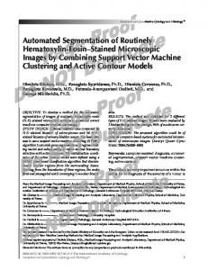
Fig. 12 illustrates an example of typical cell images.

Fig. 13 and Fig. 14 show the detected results of the images in Fig. 12 (a) and (b). Fig 15 and 16 (a) are the original images, (b) is the extracted outlines from phase I, (c) shows the detected ellipses imposed on (b), and (d) shows the detected ellipses imposed on the original images.

25


Page 26 of 41

Page 27 of 41


It can be seen, in Fig. 13 that ellipses are successfully approximated, even when several cells overlap, thus making cell segmentation possible. In Fig. 14, partial cells are also successfully approximated with ellipses. More examples of successfully segmented cells are shown in Fig. 15 and Fig. 16. And, more examples of successfully approximating partial cells are shown in Fig. 17 and Fig. 18.

However, the experiments also present some problems.

Fig. 19 shows a missed cell, which is cell A in Fig. 19 (a), due to limited outline extraction. A possible solution could be better extraction of blobs from the original image, so that the outlines are as close as possible to the originals. As Fig. 19 (a) shows, if the dark gap between cells A and B is clearly identified, the outline of cell A will not be ignored as noise.

Fig. 20 shows a similar example. If the gap A in Fig. 20 (a) is clearly identified, so that the relative completeness of the boundary of cells B and C is maintained, it is possible to separate them as two ellipses. Fig. 19 also shows two cells identified as one ellipse; ellipse C shown in Fig. 19 (d). It is impossible for cell D in Fig. 19 (b) to be identified as an independent cell because its outline does not look, remotely, as an ellipse: complete or partial. A possible solution for this kind of problem is to differentiate different cells according to color, and not just overall shape: cell D is orange in color while the others are mostly green.

Fig. 21 shows a similar example. If outlines of cell A and cell B can be separated using their color information, they should be able to be identified as two ellipses rather than one.

Fig. 22 shows another failed detection due to the mismatch between the extracted and the original outlines. The shape of the boundary is affected negatively by the shade within the cell. However, if the relatively bright area on the right side of the cell could be detected, the original outline of the cell would be maintained and thus a correct ellipse would fit it.

26



Fig. 23 also demonstrates the same problem. A small black area within the cell affects the boundary of the whole cell. If all “bight pixels” in the cells are identified correctly, then this will not be a problem.

Fig. 24 shows a missing cell due to its relatively low brightness. Only highly visible blobs are segmented in phase I. This shows that our algorithm needs better local adaptation for the threshold. And, Fig. 25 also shows a missed cell due to the relatively low threshold value. This problem occurred simply because the same threshold value is being used throughout the whole program. However, as seen below, some images need higher threshold values in order to better discern the outlines of the cells.

In summary, we have very few problems, but they prevent perfectly accurate segmentation of cells. It is possible, however, to remedy the situation by implementing the following embellishments: •

Stricter identification of the boundaries of blobs. This demands careful choice of both global and local thresholds.

•

Inclusion of color information in the criteria used to segment cells from blobs (in addition to shape information).

•

Reducing the effect of shading within blobs/cells: these can be filtered out/ blurred a little using a standard Butterworth filter.

•

Increasing the range of local thresholds by amending equation (8).

7.2 Statistical Analysis

To generate summary statistical results for phase1, we devised a number of specific measures, which are defined below. To report overall performance of phase 1, we use Accuracy, which is the ratio of the number of correctly detected blobs to the total number of blobs actually present in the target image, expressed as a percentage. %fn is the number of blobs actually present in the image but not detected by the program, expressed as a percentage of total number of cells in the image. As such accuracy added to %fn always comes to 100. On the other hand, percentage of false positive (%fp), which denotes the number of nonexistent blobs that the program detected divided by the total number of blobs, expressed as a percentage.

27


Page 28 of 41

Page 29 of 41


TABLE II PHASE1 PERFORMANCE - ACCURACY

Images

Accuracy

%fn

%fp

Class A

99.09

0.91

0.00

Class B

90.37

9.63

0.00

Overall

97.13

2.87

0.00

We then computed the number of blobs that were precisely extracted. A precisely extracted blob is one with an actual contour that matches the contour drawn by phase 1 of the program. An inaccurately identified blob is one where the actual contour is much larger (under coverage or UC) or smaller (over coverage or OC) than the contour identified by the program. Precision is the percentage of actual blobs that were properly segmented by the program. %UC is the number of blobs with under-covering programgenerated contours, divided by the total number of blobs, and expressed as a percentage. %OC is the number of blobs with over-covering program-generated contours, divided by the total number of blobs, and expressed as a percentage.

TABLE III PHASE1 PERFORMANCE - PRECISION

Images

Precision

%UC

%OC

Class A

98.53

1.47

0.00

Class B

92.36

7.64

0.00

Overall

97.14

2.86

0.00

To generate summary statistical results for phase 2, we devised a number of measures, which are defined below. To report overall performance of program CellCount (phase 1 and phase 2), we use Accuracy, which is the ratio of the number of correctly detected cells to the total number of cells actually present in the target image, expressed as a percentage. %fn is the number of cells actually present in the image but not detected by the program, expressed as a percentage of total number of cells in the image. As such accuracy

28



added to %fn always comes to 100. On the other hand, percentage of false positive (%fp), which denotes the number of non-existent cells that the program detected divided by the total number of cells, expressed as a percentage.

Table IV shows the overall performance, i.e., the average accuracy, fp as well as fn rate we have achieved:

TABLE IV OVERALL PERFORMANCE OF PROGRAM

Images

Accuracy

%fn

%fp

Class A

98.11

1.89

3.34

Class B

90.93

9.07

13.76

Overall

96.35

3.65

5.24

7.3 Conclusion

In this paper, we make a number of distinct contributions that are relevant to both shape detection and biomedical image processing.

First, we propose and use an iterative thresholding technique, which is applied to the problem of cell/cell cluster segmentation. The results of the application were good (97.13% accuracy) but not perfect. We provide a short-list of possible improvements. Nevertheless, it is our belief that the general strategy of using iteration in order to adapt to local conditions (of, for example, illumination) within an image, is one that likely to improve the quality of many foreground object extraction algorithms, with the field of image processing.

Second, we propose and use a new GA-based ellipse (circle) detection technique, which is applied to the problem of elliptical/circular cell segmentation with success (96.35% accuracy). It is worth nothing here that this ellipse detection technique has worked despite the imperfect nature of the perimeter of cells (e.g.

29


Page 30 of 41

Page 31 of 41


deformations, missing sections and the like). As such it is our belief that this ellipse detection mechanism is not only fast but also robust, and as such, is suitable for ellipse detection problems in general.

ACKNOWLEDGEMENTS

I would like to express my profound gratitude to Tasnim El-Asmar for her support and assistance in the drafting and editing of this paper. This has been a significant undertaking that she shouldered with patience and grace. I would also wish to express my thanks to Peter Grogono for his help in reviewing the details of the MPGA algorithm.

REFERENCES

[1] Anoraganingrum, D.; Kröner, S.; and Gottfried, B.; "Cell Segmentation with Adaptive Region Growing," ICIAP Venedig, Italy, 27-29 September 1999. [2] Ballard, D. H.; “Generalizing the Hough Transform to Detect Arbitrary Shapes”, Pattern Recognition, Vol. 13, No. 2, 1981, pp. 111-122. [3] Bamford, P.; Lovell, B.; "A Water Immersion Algorithm for Cytological Image Segmentation," Proceedings APRS Image Segmentation Workshop, December 13, 1996, pages 75-79, Sydney, Australia. [4] Brais, B.; Bouchard, J.P.; Xie, Y.G. ; Rochefort, D.L. ; Chretien, N. ; Tome, F.M. ; Lafreniere, R.G.; Rommens, J.M.; Uyama, E. ; Nohira, O.; et al.; “Short GCG expansions in the PABP2 gene cause oculopharyngeal muscular dystrophy, ” Nat. Genet., 18, pp. 164–167, 1998. [5] Chakraborty, S. and Deb, K.; “Analytic Curve Detection from a Noisy Binary Edge Map Using Genetic Algorithm”, PPSN, 1998, pp. 129-138. [6] Fang, B.; Hsu, W. and Lee, M.L.; “On the Accurate Counting of Tumor Cells”, IEEE Trans. Nanobioscience, Vol. 2, No. 2, June 2003, pp. 94 – 103. [7] Garrido, A.; de la Blanca, N.; "Applying deformable templates for cell image segmentation," Pattern Recogn., vol. 33, no. 5, pp. 821-832, May 2000.

30



[8] Glenner, G.G.; and Wong, C.W.; “Alzheimer’s disease and Down’s syndrome: sharing of a unique cerebrovascular amyloid fibril protein,” Biochem. Biophys. Res. Commun., 120, pp. 885-890, 1984. [9] Goldberg, D. E. and

Richardson, J.; "Genetic algorithms with sharing for multimodal function

optimization," Proceeding of the 2nd Int. Conference on Genetic Algorithms, J. J. Grefenstette, Ed. Hillsdale, NJ: Lawrence Erlbaum, 1987, pp. 41-49. [10] Grimson, W.E.L. and Huttenlocher, D.P.; “On the sensitivity of the Hough transform for object recognition”, IEEE Trans. Pattern Anal. Machine Intelli., Vol. 12, No. 3, March 1990, pp. 255-274. [11] Guil, N. and Zapata, E. L.; “Lower order circle and ellipse Hough Transform”, Pattern Recognition, Vol.30, No.10, 1997, pp.1729-1744. [12] Haralick, R. M. and Shapiro, L. G. Computer and Robot Vision, Volume I, Addison-Wesley, 1992, pp. 28-48. [13] Hearn and Baker, M. P.; Computer Graphics C Version, D., Prentice Hall, Inc., 1997. [14] Ho, C.-T. and Chen, L.-H., “A Fast Ellipse/Circle Detector Using Geometric Symmetry”, Pattern Recognition, Vol. 28, No.1, 1995, pp. 117-124. [15] Hough, P.V.C.; “Machine Analysis of Bubble Chamber Pictures”, International Conference on High Energy Accelerators and Instrumentation, CERN, 1959. [16] Jeacocke, M. B.; and Lovell, B. C.; “A multi-resolution algorithm for cytological image segmentation,” in Proc. 2nd Aust. and New Zealand Conf. Intelligent Information Systems, 1994, pp. 322– 326. [17] Lei, Y. and Wong K. C.; “Ellipse detection based on symmetry”, Pattern Recognition Letters, Vol. 20, No. 1, January 1999, pp. 41-47. [18] Lutton, E. and Martinez, P.; “A Genetic Algorithm for the Detection of 2D Geometric Primitives in Images”, Proceedings of the 12th International Conference on Pattern Recognition, Jerusalem, Israel, 9-13 October 1994, Vol. 1, pp. 526-528. [19 a] Mainzer, T.; “Genetic Algorithm for traffic sign detection”, Applied Electronic 2002. [19 b] Mainzer, T.; “Genetic Algorithm for Shape Detection”, Technical Report no. DCSE/TR-2002-06, University of West Bohemia, 2002.

31


Page 32 of 41

Page 33 of 41


[20 a] Malpica, N.; Santos, A.; Tejedor, A.; Torres, A.; Castilla, M.; Garcia-Barreno, P.; Desco, M.; “Automatic quantification of viability in epithelial cell cultures by texture analysis,” J. of Microscopy, Vol. 209, Pt 1 Jan., pp. 34-40, 2003. [20 b] Malpica, N.; de Solorzano, C. O.; Vaquero, J. J.; Santos, A.; et al.; "Applying Watershed Algorithms to the Segmentation of Clustered Nuclei," Cytometry 28: 289-297, 1997. [21] McLaughlin, R. A.; “Randomized Hough Transform: Improved ellipse detection with comparison”, Pattern Recognition Letters, Vol. 19, No. 3-4, March 1998, pp. 299–305. [22] Otsu, N.; "A Threshold Selection Method from Grey-Level Histograms," IEEE Trans. System, Man and Cybernetics, vol. 9, no. 1, pp. 377-393, 1979. [23] Press, W. H. et al., Numerical Recipes in C, The Art of Scientific Computing Second Edition, Cambridge University Press, 1992, Chapter 2, pp. 43-50. [24] Procter, S. and Illingworth, J.; “A Comparison of the Randomized Hough Transform and a Genetic Algorithm for Ellipse Detection”, Pattern Recognition in Practice IV: multiple paradigms, comparative studies and hybrid systems, edited by E Gelsema and L Kanal, Elsevier Science Ltd., pp. 449-460. [25] Roth, G. and Levine, M. D.; “Geometric primitive extraction using a genetic algorithm”, IEEE Transactions on Pattern Analysis and Machine Intelligence, Vol. 16, No. 9, September 1994, pp. 901-905. [26] Sherman, M.Y.; and Goldberg, A.L.; “Cellular defences against unfolded proteins: a cell biologist thinks about neurodegenerative diseases,” Neuron, 29, pp. 15-32, 2001. [27] Smith, R. E.; Forrest, S. and Perelson, A. S.; “Searching for diverse, cooperative populations with genetic algorithms”, TCGA Report No. 92002, The University of Alabama, Dept. of Engineering Mechanics, 1992. [28] Spann, M.; Wilson, R.; “A quadtree approach to image segmentation that combines statistical and spatial information,” Pattern Recognition, 18: 257-269, 1985. [29] Tome, F.M.S.; Fradeau, M.; “Nuclear changes in muscle disorders,” Methods Achiev Exp Pathol, 12, pp. 2261-296, 1986. [30] Woods, R.E.; and Gonzales, R.C.; “Digital Image Processing,” Reading, MA: Addison-Wesley, 1993. [31] Wu, H.; Barba, J.; and Gil, J.; "Iterative thresholding for segmentation of cells from noisy images," J. of Microscopy, vol. 197, no. 3, pp. 296-304, 2000.

32



[32] Wu, K.; Gauthier, D.; and Levine, M. D.; “Live cell image segmentation,” IEEE Trans. Biomed. Eng., vol. 42, pp. 1–12, Jan. 1995. [33] Xu, L.; Oja, E. & Kultanen, P.; “A New Curve Detection Method: Randomized Hough Transform (RHT)”, Pattern Recognition Letters, Vol. 11, No. 5, May 1990, pp. 331-338. [34] Yao, J.; Kharma, N.; and Grogono, P. “Fast Robust GA-based Ellipse Detection”, proceedings of the International Conference on Pattern Recognition, Cambridge, U.K., August 23-36, 2004. pp. 859-862. [35] Zoghbi, H.Y.; and Orr, H.T.; “Glutamine repeats and neurodegeneration,” A. Rev. Neurosci., 23, pp. 217-247, 2000.

33


Page 34 of 41

Page 35 of 41


LIST OF FIGURES

Fig. 1: An image of what neurofibrillary tangle in Alzheimer's disease looks like under the microscope.

Fig. 2: Shown is a neuron from disease brain containing a ubiquitinated intranuclear inclusion (arrow). The neuron shown is from the pons of spinocerebellar ataxia type 3 brain, but intranuclear inclusions of aggregated disease protein are a common feature of most polyglutamine diseases.

Fig. 3: Expression of mutant PABPN1-ala17 in Hela cells induces insoluble intranuclear inclusions of OPMD.

(a)

(b)

Fig. 4: Global and Local Optima. (a) A Large Imperfect Ellipse (Left) and a much Smaller Perfect Ellipse (Right). (b) Locally-Optimum Candidate Ellipse Overlaid on top of Left Ellipse.



Page 36 of 41

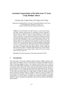
Blob Extraction Gray Scale Conversion

Application of Open Morphological Operation: Erode Dilate

Global Thresholding

Blob Labelling and Extraction: Label Pixels Extract Blobs

Multi -Region Adaptive Thresholding

Second Application of Open Morphological Operation

Second Labelling of Pixels and Extraction of Blobs

Initialize First Population

Evaluate Fitness (rank) & Select

Yes Converge?

Y

No Clustering End Evolution

Ellipse Detection Fig. 5: Overview of two-phase algorithm for blob extraction and ellipse detection for the segmentation of cells/nuclei from blobs.


Page 37 of 41


(a)

(b)

Fig. 6: Segmentation results (a) Original image containing regions of interest to be extracted. (b) Mask image.

Fig. 7: Matching of a Candidate Ellipse, Point by Point, to Potential Actual Ellipses in an Image

Fig. 8: 2D Geometric Transformation of Ellipse



Fig. 9: Result of Crossing-Over Two Chromosomes: Genotypic View

Fig. 10: Result of Crossing-Over Two Chromosomes: Phenotypic View

Fig. 11: Mutation Operation


Page 38 of 41

Page 39 of 41


(a)

(b)

Fig. 12 Typical Cell Images (a) Nonviable Cells (b) Viable Cells

(a)

(b)

(c)

(d)

Fig. 13 Segmentation Results for Fig. 12(a)

(a)

(b)

(c)

(d)

Fig. 14 Segmentation Results for Fig. 12(b)

(a)

(b)

(c)

(d)

Fig. 15 Successful Segmentation of Overlapping Cells I

(a)

(b)

(c)

(d)

Fig. 16 Successful Segmentation of Overlapping Cells II



(a)

(b)

(c)

(d)

Fig. 17 Segmentation Results of Partial Cells I

(a)

(b)

(c)

(d)

Fig. 18 Segmentation Results of Partial Cells II

A D

B

(a)

C

(b)

(c)

(d)

Fig. 19 Incorrect Segmentation of Cells I

(a)

(b)

(c)

(d)

Fig. 20 Incorrect Segmentation of Cells II

(a)

(b)

(c)

(d)

Fig. 21 Incorrect Segmentation of Cells III


Page 40 of 41

Page 41 of 41


(a)

(b)

(c)

(d)

Fig. 22 Mismatch between Extracted and Original Cell I

(a)

(b)

(c)

(d)

Fig. 23 Mismatch between Extracted and Original Cell II

(a)

(b)

(c)

(d)

Fig. 24 Missed Cell Due to Local Thresholding Effects I

(a)

(b)

(c)

(d)

Fig. 24 Missed Cell Due to Local Thresholding Effects II


Automatic Segmentation of Cells from Microscopic Imagery using ...

Automatic Segmentation of Cells from Microscopic Imagery using ...

Suggest Documents

Automatic Detection of Buildings and Trees from Aerial Imagery Using ...

Automatic Image Segmentation using Threshold

Automatic Brain Tumor Segmentation using

Automatic Coronary Artery Segmentation Using

Automatic Road Centerline Extraction from Imagery Using ... - MDPI

Automatic Segmentation of Parotids from CT Scans Using Multiple

automatic segmentation of coronary arteries using ... - CiteSeerX

AUTOMATIC SEGMENTATION OF BUILDING FACADES USING

automatic segmentation of mammographic masses using ... - CiteSeerX

automatic segmentation of mammographic masses using ... - CiteSeerX

Supplementary Information Automatic Segmentation of Kidneys using ...

Semi-automatic Metadata Extraction from Imagery

Automatic Segmentation of Blood Vessels from ...

Automatic Liver Segmentation from CT Images Using Single-Block ...

Semantic Segmentation of Underwater Imagery Using Deep Networks

Automatic segmentation of

Confidence-Based Segmentation of MR Imagery Using ... - Grinnell CS

Automatic Frequency Band Segmentation Using Statistical Similarity ...

Automatic Discourse Segmentation using Neural Networks - CiteSeerX

Automatic nevi segmentation using adaptive ... - Computing Science

Automatic lithofacies segmentation using the Wavelet Transform ...

Automatic Subcortical Segmentation Using a Novel ... - CiteSeerX

Automatic Brain Segmentation Using Artificial Neural ... - MRBrainS

Automatic image segmentation using a deformable