Automatic Segmentation of MS Lesions Using a Contextual Model for ...

Automatic Segmentation of MS Lesions Using a Contextual Model for the MICCAI Grand Challenge Jonathan H. Morra1 , Zhuowen Tu1 , Arthur W. Toga1 , Paul M. Thompson1

July 14, 2008 1 Laboratory

of Neuro Imaging, UCLA School of Medicine, Los Angeles, CA, USA Abstract

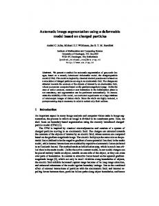
Automatically segmenting subcortical structures in brain images has the potential to greatly accelerate drug trials and population studies of disease. Here we propose an automatic subcortical segmentation algorithm using the auto context model. Unlike many segmentation algorithms that separately compute a shape prior and an image appearance model, we develop a framework based on machine learning to learn a unified appearance and context model. In order to test the method, specificity and sensitivity measurements were obtained on a standardized dataset provided by the competition organizers. Our overall score of 77 seems to be competitive with others who’s overall score was in the range of 50 - 90.

1

Introduction

Segmentation of subcortical structures on brain MRI is vital for many clinical and neuroscientific studies. In many studies of brain development or disease, subcortical structures must typically be segmented in large populations of patients and healthy controls, to quantify disease progression over time, to detect factors influencing structural change, and to measure treatment response. In brain MRI, MS lesions are structures of great neurological interest, but are difficult to segment automatically. 3D medical image segmentation has been intensively studied. Most approaches fall into two main categories: those that design strong shape models [1, 13, 5] and those that rely more on strong appearance models (i.e., based on image intensities) or discriminative models [2, 7]; atlas-based, shape-driven and other segmentation methods were recently compared in a caudate benchmark test [12]; despite the progress made, no approach is yet widely used due to (1) slow computation, (2) unsatisfactory results, or (3) poor generalization capability. In object and scene understanding, it has been increasingly realized that context information plays a vital role [4]. Medical images contain complex patterns including features such as textures (homogeneous, inhomogeneous, and structured) which are also influenced by acquisition protocols. The concept of context covers intra-object consistency (different parts of the same structure) and inter-object configurations (e.g., expected symmetry of left and right hemisphere structures). Here we integrate appearance and context information in a seamless way by automatically incorporating a large number of features through iterative procedures. The resulting algorithm has almost identical testing and training procedures, and segments images rapidly by avoiding an explicit energy minimization step. We train and test our model on a dataset provided by

2

the MICCAI Grand Challenge II workshop for segmenting MS lesions. For a validation of the presented method on hippocampal and caudate segmentation please refer to [3].

2 2.1

Methods Problem

The goal of a subcortical image segmenter is to label each voxel as belonging to a specific region of interest (ROI), such as an MS lesion. Let X ∈ (x1 . . . xn ) be a vector encompassing all N voxels in each manuallylabeled training image and Y ∈ (y1 . . . yN ) be the label for each example, with yi ∈ 1 . . . K representing one of K labels (for hippocampal segmentation, this reduces to a two-class problem). According to Bayesian probability, we look for the segmentation

Y ∗ = argmax p(Y |X) = argmax p(X|Y )p(Y ) Y ∈K

Y ∈K

where p(X|Y ) is the likelihood and p(Y ) is the prior distribution on the labeling Y . However, this task is very difficult. Traditionally, many “bottom-up” computer vision approaches (such as SVMs using local features [7]) work hard on directly learning the classification p(Y |X) without encoding rich shape and context information in p(Y ), whereas many “top-down” approaches such as deformable models, active surfaces, or atlas-deformation methods impose a strong prior distribution on the global geometry and allowed spatial relations, and learn a likelihood p(X|Y ) with simplified assumptions. Due to the intrinsic difficulty in learning the complex p(X|Y ) and p(Y ), and searching for the Y ∗ maximizing the posterior, these approaches have achieved limited success. Instead, we attempt to model p(Y |X) directly by iteratively learning the marginal distribution p(yi |X) for each voxel i. The appearance and context features are selected and fused by the learning algorithm automatically. 2.2

Auto Context Model

A traditional classifier can learn a classification model based on local image patches, which we now call (0)

(0)

(0)

Pk = (Pk (1), ..., Pk (n)) (0)

where Pk (i) is the posterior marginal for label k at each voxel i learned by a classifier (e.g., boosting or SVM). We construct a new training set S1 = {(yi , X(Ni ), P(0) (Ni )), i = 1..n}, where P(0) (i) are the classification maps centered at voxel i. We train a new classifier, not only on the features from the image patch X(Ni ), but also on the probability patch, P(0) (Ni ), of a large number of context voxels. These voxels may be either near or very far from i. It is up to the learning algorithm to select and fuse important supporting context voxels, together with features about image appearance. For our purposes, our feature pool consisted of 18,099 features including intensity, position, and neighborhood features. Our

3

neighborhood features were mean filters, standard deviation filters, curvature filters, and gradients of size 1x1x1 to 3x3x3, and Haar filters of various shapes from size 2x2x2 to 7x7x7. Our AdaBoost weak learners were decision stumps on both the image map and probability map. Once a new classifier is learned, the algorithm repeats the same procedure until it converges. The algorithm iteratively updates the marginal distribution to approach (n)

(n−1)

p (yi |X(Ni ), P

(Ni )) → p(yi |X) =

Z

p(yi , y−i |X)dy−i .

(1)

In fact, even the first classifier is trained the same way as the others by giving it a probability map with a uniform distribution. Since the uniform distribution is not informative at all, the context features are not selected by the first classifier. In some applications, e.g. medical image segmentation, the positions of the anatomical structures are roughly known after registration to a standard atlas space. One then can provide a probability map of the structure (based on how often it occurs at each voxel) as the initial P(0) . Given a set of training images together with their label maps, S = {(Y j , X j ), j = 1..m}: For (0)

each image X j , construct probability maps P j , with a distribution (possibly uniform) on all the labels. For t = 1, ..., T : (t−1)

• Make a training set St = {(y ji , X j (Ni ), P j

(Ni )), j = 1..m, i = 1..n}.

• Train a classifier on both image and context features extracted from X j (Ni ) and (t−1)

Pj

(Ni ) respectively. (t)

• Use the trained classifier to compute new classification maps P j (i) for each training image X j .

The algorithm outputs p(n) (yi |X(Ni ), P(n−1) (Ni ))

a

sequence

of

trained

classifiers

for

Figure 1: The training procedures of the auto-context algorithm. We can prove that at each iteration, ACM is decreasing the error εt . If we note that the error of one example (i), at time t − 1 is P(t−1) (i)(yi ) and at time t is pt (yi |Xi , P(t−1) (i)), then we can use the log-likelihoods to formulate the error over all examples as in eqn. 2.

εt−1 = − ∑i log P(t−1) (i)(yi ), εt = − ∑i log p(t) (yi |Xi , P(t−1) (i))

(2)

First, it is trivial to choose p(t) to be a uniform distribution, making εt = εt−1 . However, boosting (or any other effective discriminative classifier) is guaranteed to choose weak learners to create p(t) that minimize εt and will fail if none such exists, so therefore, if AdaBoost completes, εt ≤ εt−1 .

3 3.1

Specifics Preprocessing and Postprocessing

Before any segmentation model was created, two preprocessing steps were performed. First the data was downsampled to 256x256x256 using a nearest neighbor interpolation. This was done to drastically speed up processing time. Secondly the data was run through a bias field corrector (BFC) [8] in order to remove the

3.2

Feature Pool and Weak Learner Description

4

bias introduced by the scanner. The only post processing done was a nearest neighbor upsample to return the mask to 512x512x512 space. 3.2

Feature Pool and Weak Learner Description

When running AdaBoost, one must first define a pool of potentially informative features to draw from. First, (0) we defined an initial shape prior (P j ), based on the LogOdds formulation of Pohl et. al [6]. Next, we used the same set of features drawn from each of these six channels (T1, T2, FLAIR, DTI-MD, DTI-FA, prior) including intensity, mean filters, standard deviation filters, curvature filters, and haar filters of various shapes. For each of the neighborhood based features, the neighborhood ranged from 1x1x1 to 7x7x7. Additionally, we used features based on the x,y,z position of each voxel. A crucial part of AdaBoost is the definition of the weak learners. In our implementation, our weak learners are decision stumps. Therefore, each weak learner consists of a feature, a threshold, and a boolean stating whether positive examples are below or above that threshold. It is also interesting to note which are the most important features selected for further analysis. For our model, the first ten features chosen (those that contributed most to the decision rule), are summarized in table 1. Feature No. 1 2 3 4 5 6 7 8 9 10

Channel FLAIR Prior FLAIR FLAIR Prior DTI-MD FLAIR FLAIR DTI-FA FLAIR

Feature Type Mean Intensity Curvature Curvature Intensity Mean Curvature Curvature Mean Curvature

Neighborhood Size 4,2,7 N.A. 6,7,5 7,7,2 N.A. 3,2,1 6,7,5 7,7,2 4,6,4 7,7,2

Table 1: The first ten features selected by AdaBoost. These contributed most to the classification rule. It is interesting to note that the FLAIR image appears the most, which is to be expected as FLAIR provides the best deliniation of MS lesions. However, it is not the only modality present. The prior image represents the LogOdds shape prior, which is also expected to be informative because is it a combination of all the training masks.

3.3

Probabilistic Boosting Tree

In order to increase the classification ability of our algorithm, instead of just using AdaBoost during each iteration of ACM, we instead made a probabilistic boosting tree (PBT) [9]. The PBT has been shown to be an effective medical image classifier [10]. We used a very small tree (due to time constraints), with a depth of only 1. Finally, we set ε (as defined in [9]) to a value of 0.1.

3.4

Randomizations

3.4

Randomizations

5

Due to the large size of our dataset and the large number of features we have available, we must scale down our training set to a manageable size. In order to do this, at each run of AdaBoost, we choose a random set of 100,000 examples to train on and a random set of 5,000 features to comprise our feature pool. However, since we are running AdaBoost many times (we used an ACM depth of 6, for a total of 18 AdaBoost runs), these randomizations are acceptable.

4

Results

Fig. 4 presents our results from the competition. For this competition we choose to train two models, one for just the UNC dataset, and one for just the CHB dataset. Ground Truth All Dataset

UNC Rater CHB Rater STAPLE Volume Diff. Avg. Dist. True Pos. False Pos. Volume Diff. Avg. Dist. True Pos. False Pos. Total Specificity Sensitivity [%] Score [mm] Score [%] Score [%] Score [%] Score [mm] Score [%] Score [%] Score UNC test1 Case01 3.3 100 10.6 78 41.9 75 47.8 80 51.0 93 8.0 84 43.8 76 43.5 83 84 0.9676 0.4061 UNC test1 Case02 232.0 66 4.7 90 41.2 75 55.8 76 56.2 92 3.0 94 31.8 70 28.8 92 82 0.9612 0.5045 UNC test1 Case03 33.1 95 2.8 94 27.5 67 25.5 94 13.5 98 2.2 96 30.9 69 14.9 100 89 0.9731 0.4461 UNC test1 Case04 38.2 94 5.4 89 36.8 72 36.4 87 4.1 99 3.8 92 55.6 83 40.9 85 88 0.9725 0.4162 UNC test1 Case05 93.5 86 19.9 59 14.3 60 14.3 100 85.4 87 17.3 64 21.7 64 28.6 92 77 0.9993 0.0657 UNC test1 Case06 92.3 86 30.2 38 13.8 59 40.0 85 65.8 90 28.2 42 25.0 66 40.0 85 69 0.9986 0.0794 UNC test1 Case07 100.0 85 128.0 0 0.0 51 0.0 100 100.0 85 128.0 0 0.0 51 0.0 100 59 1.0000 0.0000 UNC test1 Case08 55.6 92 9.8 80 14.9 60 14.3 100 27.5 96 4.0 92 38.9 74 14.3 100 87 0.9921 0.3265 UNC test1 Case09 140.8 79 49.4 0 0.0 51 100.0 49 239.7 65 56.7 0 0.0 51 100.0 49 43 0.9770 0.1875 UNC test1 Case10 219.8 68 19.4 60 15.0 60 78.6 62 1056.1 0 21.9 55 33.3 70 85.7 57 54 0.9478 0.4613 CHB test1 Case01 179.0 74 5.1 90 40.0 74 48.1 80 298.7 56 5.4 89 77.4 95 57.7 74 79 0.9585 0.6623 CHB test1 Case02 307.6 55 7.7 84 50.0 80 73.1 65 73.7 89 1.5 97 63.2 87 46.2 82 80 0.9281 0.8002 CHB test1 Case03 53.9 92 7.9 84 64.3 88 82.4 59 25.6 96 7.1 85 53.3 82 74.3 64 81 0.9807 0.2692 CHB test1 Case04 331.7 51 8.0 84 90.9 100 77.8 62 107.6 84 2.3 95 83.3 99 51.9 78 82 0.9538 0.7524 CHB test1 Case05 936.8 0 10.6 78 51.9 81 80.3 61 96.7 86 2.0 96 78.3 96 59.1 74 71 0.9327 0.7187 CHB test1 Case06 24.0 96 2.9 94 41.7 75 70.7 67 20.6 97 2.7 94 36.4 72 72.0 66 83 0.9825 0.4682 CHB test1 Case07 138.9 80 5.2 89 48.3 79 52.6 78 45.4 93 1.4 97 47.4 78 55.3 76 84 0.9529 0.8110 CHB test1 Case08 227.1 67 3.5 93 77.8 96 64.9 70 118.9 83 2.2 96 61.8 87 45.9 82 84 0.9125 0.8382 CHB test1 Case09 335.3 51 4.2 91 43.6 76 74.4 64 267.1 61 3.3 93 34.6 71 73.1 65 72 0.8113 0.8395 CHB test1 Case10 497.9 27 7.2 85 78.9 96 82.9 59 192.4 72 2.7 95 79.3 97 70.0 67 75 0.9228 0.6613 CHB test1 Case11 389.2 43 6.8 86 36.4 72 88.1 56 58.2 91 2.5 95 37.9 73 73.8 65 73 0.9381 0.6976 CHB test1 Case12 74.6 89 5.7 88 15.7 60 28.3 92 74.8 89 5.5 89 23.1 65 26.4 94 83 0.9941 0.2456 CHB test1 Case13 160.1 77 10.3 79 80.0 97 81.4 60 59.4 91 3.0 94 85.7 100 58.1 74 84 0.9040 0.5411 CHB test1 Case15 24.1 96 2.5 95 52.1 81 33.9 89 63.6 91 2.0 96 57.4 84 50.8 79 89 0.9373 0.7442 All Average 195.4 73 15.3 75 40.7 74 56.3 75 133.4 83 13.2 80 45.8 78 50.5 78 77 0.9541 0.4976 All UNC 100.9 85 28.0 59 20.5 63 41.3 83 169.9 81 27.3 62 28.1 67 39.7 84 73 0.9789 0.2893 All CHB 262.9 64 6.3 87 55.1 83 67.1 69 107.3 84 3.1 94 58.5 85 58.2 74 80 0.9364 0.6464

PPV 0.3708 0.6590 0.4779 0.5548 0.7925 0.7852 nan 0.5421 0.1581 0.2433 0.2872 0.3630 0.1785 0.4596 0.3616 0.6543 0.5664 0.3391 0.2410 0.2953 0.3831 0.7742 0.2523 0.5721 0.4483 0.5093 0.4091

Figure 2: The competition results for our segmentation algorithm. For an overview of the meaning of these metrics, refer to last year’s competition [11]. For most images, a reasonable segmentation is found, and a good score is achieved. There are only a few outliers which our system did not segment well, cases 7, 9, and 10 in the UNC test case seem to do the poorest, however, most other cases do very well, in fact there is no overall score in the CHB dataset which is below 71.

5

Conclusions

Our method finds a reasonable segmentation on most images, and the results of fig. 4 show that for most cases the segmentation is relatively good. At the time of writing we do not know the score of the other

6

groups, but only know the range of total scores is between 50 and 90, and our score of 77 seems very acceptable, especially when considering this system was originally designed to segment subcortical structures such as the hippocampus and caudate.

6

Acknowledgements

Grant support for this work was provided by the National Institute for Biomedical Imaging and Bioengineering, the National Center for Research Resources, National Institute on Aging, the National Library of Medicine, and the National Institute for Child Health and Development (EB01651, RR019771, HD050735, AG016570, LM05639 to P.M.T.) and by the National Institute of Health Grant U54 RR021813 (UCLA Center for Computational Biology). L.G.A. was also supported by NIA K23 AG026803 (jointly sponsored by NIA, AFAR, The John A. Hartford Foundation, the Atlantic Philanthropies, the Starr Foundation and an anonymous donor) and NIA P50 AG16570.

References [1] B. Fischl et al. Whole brain segmentation: Automated labeling of neuroanatomical structures in the human brain. Neurotechnique, 33:341–355, 2002. [2] R. A. Heckemann, J. V. Hajnal, P. Aljabar, D. Rueckert, and A. Hammers. Automatic anatomical brain MRI segmentation combining label propagation and decision fusion. Neuroimage, 33(1):115–126, October 2006. [3] J.H. Morra, Z. Tu, L.G. Apostolova, A.E Green, A.W. Toga, and P.M. Thompson. Automatic subcortical segmentation using a contextual model. In MICCAI, 2008. [4] A. Oliva and A. Torralba. The role of context in object recognition. Trends in Cognitive Sciences, 11(12):520–527, December 2007. [5] K.M. Pohl, J. Fisher, R. Kikinis, W.E.L. Grimson, and W.M. Wells. A Bayesian model for joint segmentation and registration. NeuroImage, 31(1):228–239, 2006. [6] K.M. Pohl, J. Fisher, M. Shenton, R.W. McCarley, W.E.L. Grimson, R. Kikinis, and W.M. Wells. Logarithm odds maps for shape representation. In MICCAI, 2006. [7] S. Powell, V.A. Magnotta, H. Johnson, V.K. Jammalamadaka, R. Pierson, and N.C. Andreasen. Registration and machine learning based automated segmentation of subcortical and cerebellar brain structures. NeuroImage, 39(1):238–247, January 2008. [8] D.W. Shattuck, S.R. Sandor-Leahy, K.A. Schaper, D.A. Rottenberg, and R.M. Leahy. Magnetic resonance image tissue classification using a partial volume model. Neuroimage, 13:856–876, 2001. [9] Z. Tu. Pobabilistic boosting tree: Learning discriminative models for classification, recognition, and clustering. In Proceedings of ICCV, 2005. [10] Z. Tu, K. Narr, I. Dinov, P. Doll´ar, P. Thompson, and A. Toga. Brain anatomical structure parsing by hybrid discriminative/generative models. IEEE TMI, 2008.

References

7

[11] B. van Ginneken, T. Heimann, , and M. Styner. 3D segmentation in the clinic: A grand challenge, workshop at medical image computing and computer assisted intervention. In MICCAI, pages 7 – 15, 2007. [12] B. van Ginneken, T. Heimann, and M. Styner. 3D Segmentation in the Clinic: A Grand Challenge. Proc. of MICCAI Workshop, 2007. [13] J. Yang, L. H. Staib, and J. S. Duncan. Neighbor-constrained segmentation with level set based 3D deformable models. IEEE TMI, 23(8):940–948, August 2004.