Automatic Testcase Synthesis and Performance Model Validation for High-Performance PowerPC Processors Robert H. Bell, Jr.†‡ Rajiv R. Bhatia†‡ Lizy K. John‡ Jeff Stuecheli†‡ John Griswell† Paul Tu† Louis Capps† Anton Blanchard† Ravel Thai‡ Technical Contact: Alex Mericas† †
IBM Systems and Technology Division Austin, Texas
[email protected] ABSTRACT The latest generation of high-performance IBM PowerPC microprocessors, the POWER5 chip, poses challenges to performance modeling, model simulation, and performance model validation efforts. To achieve accurate performance projections, the performance models for this high-performance processor must be written at a very detailed level, which reduces the efficiency of the model simulation. The detail also exacerbates the problem of performance model validation, which seeks to execute codes and compare results between performance models and hardware or functional models built from hardware descriptions of the machine. The current state-of-the-art is to use simple hand-coded bandwidth and latency testcases, but these are not comprehensive for processors as complex as the POWER5 chip. Applications and benchmark suites such as SPEC CPU are difficult to set up or take too long to execute on functional models or even on detailed performance models. We present an automatic testcase synthesis methodology to address these concerns. By basing testcase synthesis on the workload characteristics of an application, source code is created that largely represents the performance of the application, but which executes in a fraction of the runtime. We synthesize representative PowerPC versions of the SPEC2000, STREAM, TPC-C and Java benchmarks, compile and execute them, and obtain an average IPC within 2.4% of the average IPC of the original benchmarks and with many similar average workload characteristics. The synthetic testcases often execute two orders of magnitude faster than the original applications, typically in less than 300K instructions, making performance model validation for today’s complex processors feasible.
1. INTRODUCTION Modern high-performance microprocessors are quite complex. For example, the POWER4™ and POWER5™ chips are dual-core PowerPC® microprocessors used in IBM server systems [32][28]. The POWER4 chip is built from 1.5 million lines of VHDL and 174 million transistors [20], and the POWER5 chip contains 276 million transistors [28]. Their designs drives detail and complexity into the performance models used for performance projections. For complex chips, it is important that the performance models be validated [7] against cycle-accurate functional
‡
Department of Electrical and Computer Engineering The University of Texas at Austin
[email protected] models during the design process in order to minimize incorrect design decisions due to inaccurate performance models. As complexity increases, the gap in accuracy can grow quickly, so validation is needed more frequently. While the relative error of design changes based on inaccurate performance models is often similar to the relative error using accurate models [7][12], subtle instruction interactions in the POWER4 and POWER5 chips necessitate very accurate performance models. Prior validation efforts have focused on bandwidth and latency tests, resource limit tests, or micro-tests [8][31][5][23] [22][21][16]. These tests are usually hand-written microbenchmarks that validate the basic processor pipeline latencies, cycle counts of individual instructions, cache hit and miss latencies, pipeline issue latencies for back-to-back dependent operations, and pipeline bypassing. Black and Shen describe automatic testcases created with up to 100 random instructions [5], not enough to approximate many workload characteristics. Desikan et al. use microbenchmarks to validate the Alpha 21267 to 2% error [11]. However, the validated simulator still gives errors from 20% to 40% on the SPEC2000 applications. Applications themselves cannot be used for performance model validation because of their impossibly long simulation runtimes [7]. In [36], only one billion functional model simulated cycles per month are obtained. In [20], farms of machines provide many simulated cycles in parallel, but individual tests on processor models execute orders of magnitude slower than hardware emulator speeds of 2500 cycles per second. Trace sampling techniques such as SimPoint [27] and SMARTS [35] can reduce runtimes in simulators, but the executions still amount to tens of millions of instructions. Statistical simulation [9][24][12] can further reduce the necessary trace lengths, but executing traces on functional models or hardware is difficult. Sakamoto et al. present a method to create a binary image of a trace along with a memory dump and execute those on a specific machine and a logic simulator [26], but there is no attempt to reduce trace lengths. Hsieh and Pedram synthesize instructions for power estimation [14], but there is no attempt to maintain the machineindependent workload characteristics necessary to represent the original applications [1][13]. Bell and John [2][5][4] synthesize C-code programs from reduced synthetic traces generated from the workload characteristics of executing applications, as in statistical simulation. The low-level workload characteristics of the
original application are retained by instantiating individual operations as volatile asm calls. The synthetic testcases execute orders of magnitude faster than the original workloads while retaining good performance accuracy. That work shows an average IPC within 2.4% of the IPC of the original Alpha applications. In this work, the synthesis effort is broadened to support high-performance PowerPC processors such as the POWER4 and POWER5 chips. The specific contributions of this paper are the following: i) The synthesis system is extended to include the PowerPC instruction set. ii) Current synthesis techniques are extended and new techniques are presented that are necessitated by the features of the POWER5 chip, including new memory access models. iii) We present two performance model validation approaches and give validation results using the testcases for a PowerPC processor. The rest of this paper is organized as follows. Section 2 presents the conceptual framework of the testcase synthesis method and some of its benefits. Section 3 describes the synthesis approach in detail. Section 4 presents experimental synthesis results for the POWER5 processor. Section 5 presents validation results for a follow-on PowerPC processor. The last sections present conclusions and references.
2. REPRESENTING COMPLEXITY As described in [3][4], representative testcase synthesis is achieved using the workload characterization and statistical flow graph of statistical simulation [12][1]. A walk of the statistical flow graph produces a synthetic trace which, when combined with memory access and branching models, is instantiated as a C-code envelope around a sequence of asm calls - a simple but flexible testcase. When the synthetic is executed, the proportions of the instruction sequences are similar to the proportions of the same sequences in the original executing application, but the number of times the sequence is executed is significantly reduced, so that the total number of instructions executed and, therefore, overall runtime are much reduced. By repeating the execution of the sequences a small number of times, convergence of memory access and branching model behavior is assured, usually in less than 300K instructions [3][4]. Because the synthetic is composed of C-code, albeit with low-level calls to, in this case, PowerPC instructions, it can be compiled and executed on a variety of performance and functional simulators, emulators, and hardware that support the ISA. The relatively small number of instructions and the flexibility of the source code make the synthetics useful for accurate performance model validation [3][4]. In the case of the POWER5 chip, executions of a cycle-accurate model built directly from the functional VHDL hardware description language model [34][20] can be compared against the detailed M1 performance model [17][16] used for performance projections. In this work, we demonstrate the flexibility of the synthetic testcases by synthesizing specifically for POWER5 chip execution and then using them to validate an improved PowerPC processor.
2.1 Performance Model The IBM PowerPC performance modeling environment is trace-driven to reduce modeling and simulation overhead [23]
Synthetic Benchmark (PowerPC C-code)
Convert to VHDL Input Format
M1 Performance Model Execution
Interpret into Trace of Completed Instructions
VHDL Model Execution
Completed Instruction Information
Instruction-byInstruction Comparison
Completed Instruction Information
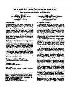
Figure 1. RTL Validation Methodology
[18][16]. The M1 performance model implements a detailed, cycle-accurate core. Coupled with the M1 is a detailed model of the L2, L3 and memory [16]. Elements of a high-performance PowerPC model must capture the functional details of the processor. The POWER5 chip features out-of-order instruction execution, two fixed point and two floating point units, 120 general purpose rename registers, 120 floating point rename registers, complex pipeline management, 32-entry load and store reorder queues, on-board L2 controller and 1.9-MB cache, L3 cache controller, 36-MB off-chip victim L3, memory controller, SMP fabric bus interface, dynamic power management, and support for simultaneous multithreading [28]. Table 6 gives additional configuration parameters.
2.2 Model Validation The POWER5 performance model was validated to within 1% for particular codes [16]. However, it is a difficult and time consuming proposition to validate a model for a large variety of programs. Automatic testcase synthesis addresses this concern by automating the synthesis process and by synthesizing high level codes that can target various platforms. In this work we target two platforms for validating the performance model: cycle-accurate RTL model simulation and simulation on a hardware emulator.
2.2.1 Validation using RTL Simulation Figure 1 shows the RTL validation methodology. The synthetic testcase is compiled and converted to execute on a VHDL model using the standard IBM functional verification simulation methodology [34][20]. The converted code is then executed to completion on the VHDL model. The compiled testcase is also unrolled into a trace using a PowerPC instruction interpreter [23][18][6]. Only completed instructions are maintained in the trace. The trace is then executed to completion on the M1 performance model. Both VHDL and performance model executions generate information at the level of the instruction, including the cycle the instruction completes, address and opcode. The cycles at which an instruction completes in both the VHDL and performance models are not identical in an absolute sense because of how cycles are maintained and counted in the two simulators. However, the performance model is of sufficient detail such that the completion cycle of an instruction minus the completion cycle of the previous instruction, that is, the cycle difference between any two completing instructions, should be equivalent. The analysis relies on the fact that the methodology generates instructions for both models from a compilation of a
single piece of code. Each and every instruction is executed on both the VHDL and M1 models and completes in the same order in both. Instructions may complete in different completion buffers in the same cycle, but should complete in the same cycle. The instantaneous error, E, for each instruction is defined in terms of the difference in cycles between the completion time of the current instruction and the completion time of the previous instruction in both VHDL and M1 models. The instantaneous error for the ith instruction is defined as:
E (i) = DR (i) − DP (i )
Statistical Simulation to Verify Trace Representativeness
User parms: instruction mix factors, stream treatment
Available Machine Registers
Machine Instruction Format
Synthetic Pisa Trace Workload Characterization
Graph Analysis
Register Assignment
Code Generation
Synthetic Alpha
Application Synthetic PowerPC
1B Instructions
where
300K Instructions Execution Comparison
DR (i ) = CR (i ) − CR (i − 1) and likewise
DP (i ) = CP (i ) − CP (i − 1) In these equations, CR(i) is the completion cycle of the ith instruction when executing the VHDL (RTL) model, and CP(i) is the completion cycle of the ith instruction when executing the M1 (Performance) model. The intuition behind the E calculation is that an instruction is using the same machine resources and completing in the same order, putatively in the same cycle, in both models, so differences between sequential instructions should be identical. A difference indicates that resource allocations or execution delays are not modeled similarly. Note that instruction dependences and resource usages using the same workload in both models will limit the instantaneous error and push it toward zero; there can be no large accumulation of error between any two related instructions. However, the completion time of an instruction that is modeled properly may be underestimated if an older instruction in program order fails to complete on time and the younger instruction is not dependent on the older but on a prior instruction and has been ready to complete for some time. The instantaneous errors can be categorized to narrow down the search for microarchitectural bugs in which a hardware feature was not implemented properly, and modeling, abstraction, and specification errors [5] in the performance model. Section 5 gives an example analysis.
2.2.2 Validation using a Hardware Emulator The compiled synthetic testcases can also be input to an RTL model executing on the AWAN hardware accelerator [20]. AWAN is composed of programmable gate arrays and can be configured to emulate a VHDL model. The AWAN array supports very large chips. The entire POWER4 chip, for example, can be emulated at a rate of more than 2500 cycles per second [20]. The cycle counts for a run are obtained from AWAN registers and compared to the M1 performance model cycle counts. Detailed workload execution information can be obtained from the AWAN machine. In Section 5, validation results using AWAN are presented.
3. SYNTHESIS FOR POWERPC With reference to Figure 2, the following sections detail the four major phases of synthesis: workload characterization; graph analysis; register assignment and code generation. In this paper, we present only the changes to the synthesis process to support the PowerPC instruction set and the high-performance processors. Additional synthesis detail, as well as exact synthesis parameters and algorithms for Pisa and Alpha code targets, can be found in Bell and John [2][3].
Figure 2: Synthesis and Simulation Overview
3.1 Workload Characterization A profile of the dynamic execution of an application produces a set of workload characteristics [3]. This is the same analysis that gives good statistical simulation correlation [12][1]. The most significant characteristics are the basic block instruction sequences and the instruction dependences [1], but we also characterize the branch predictabilities and the L1 and L2 I-cache and D-cache miss rates at the granularity of the basic block. Instructions are abstracted into five classes plus subtypes: integer, floating-point (short or long execution times, and extremely long execution times for PowerPC fma operations), load (integer or float), store (integer or float), and branch (on integer or float). The workload characterization process results in a statistical flow graph [12][1]. There is no separate input dataset for the synthetic testcases. The input dataset manifests itself in the final workload characteristics obtained from the execution profile. While separate testcases must be synthesized for each possible dataset, the automatic synthesis approach makes that feasible.
3.2 Graph Analysis In the following sections, the analysis of the statistical flow graph for code synthesis is described. The synthesis properties in Table 4 and the factors in Table 5 are described.
3.2.1 Instruction Miss Rate and I-cache Model The number of basic blocks to be instantiated in the synthetic testcase is estimated based on a default I-cache size and configuration. We then tune the number of synthetic basic blocks to match the original I-cache miss-rate (IMR). Specific basic blocks are chosen from a walk of the statistical flow graph, as in [12][1]. The IMR sometimes changes after the branches are configured in the branching model (Section 3.2.5). To compensate, the branch jump granularity is adjusted to change the number of basic blocks or instructions that a configured branch jumps. Usually a small number of synthesis iterations are necessary to match the IMR. The numbers of basic blocks and instructions synthesized for the PowerPC versions of the SPEC2000 and STREAM benchmarks are shown in Table 4.
3.2.2 Instruction Dependences and Compatibility All instruction input dependences are assigned. The starting dependence is exactly the dependent instruction chosen as an input during statistical simulation. The issue then becomes operand compatibility: if the dependence is not compatible with
the input type of the dependent instruction, then another instruction must be chosen. The algorithm is to move forward and backward from the starting dependence through the list of instructions in sequence order until the dependence is compatible. In our PowerPC experiments, some benchmarks had high average numbers of moves away from the starting dependence. To compensate, after 25 moves, a compatible instruction is inserted into the basic block near the starting dependence. The total number of inserts for each benchmark is shown in the dependence inserts column of Table 4. The highest numbers are associated with mgrid and applu, which have the largest average basic blocks sizes, at 125 and 115 respectively. Interestingly, gcc, which has a small average basic block size, still needs inserts due to long sequences of branches without sufficient intervening instructions for dependences. Using the inserts, the average number of moves per instruction input, shown in column dependence moves, is generally small. In the case of a store or branch that is operating on external data for which no other instruction in the synthetic instructions is compatible, an additional variable of the correct data type is created. Table 1 shows the compatibility of instructions for the PowerPC instruction set. The Inputs column gives the assembly instruction inputs that are being tested for compatibility. For loads and stores, the memory access register must be an integer type. When found, it is attributed as a memory access counter (LSCNTR) for special processing during the code generation phase. The PowerPC fma operations have three input operands. In some cases, the dependence factor in Table 5 is used to multiply the synthetic dependences to more closely match the overall averages in the original application. The dependence adjustment for mgrid was necessary due to its large average basic block size and, therefore, small number of synthetic basic blocks.
3.2.3 Loop Counters and Program Termination When all instructions have compatible dependences, a search is made for an additional integer instruction that is attributed as the loop counter (BRCNTR). The branch in the last basic block in the program checks the BRCNTR result to determine when the program is complete. The number of executed loops, loop iterations in Table 4, is chosen to be large enough to assure IPC convergence. Conceptually, this means that the number of loops must be larger than the longest memory access stream pattern of any memory operation among the basic blocks. In practice, the number of loops does not have to be very large to characterize simple stream access patterns. Experiments have shown that the product of the loop iterations and the number of instructions must be around 300K to achieve low branch predictabilities and good stream convergence. The loop Table 1. PowerPC Dependence Compatibility Chart Dependence Dependent Comment Inputs Compatibility Instruction Integer Float LoadInteger/Float Store-Integer Store-Float StoreInteger/Float Branch
0/1 0/1/2 0 0 0 1 0/1
Integer, Load-Integer Float, Load-Float 3 Inputs for fma Memory access Integer counter input Integer, Load-Integer Data input Float, Load-Float Data input Memory access Integer counter input Integer, Load-Integer Condition Registers
iterations are therefore approximately 300K/(number of instructions). This can be tuned with a user parameter. An mtspr instruction initializes the internal count register to the loop iterations, and the final branch checks for zero in the count register and decrements it.
3.2.4 Memory Access Model The LSCNTR instructions are assigned a stride based on the D-cache hit rate found for their corresponding load and store accesses during workload characterization. The memory accesses for data are modeled using the stream access classes shown in Table 2. The stride assignment for a memory access is determined first by matching the L1 hit rate of the load or store fed by the LSCNTR, after which the L2 hit rate for the stream is determined. The first two rows are only useful for stores in store-through POWER machines. Stores in the L2 gather such that a simple walk through memory results in a 50% L2 hit rate. If the L1 hit rate is below 3.17%, the L2 hit rate is matched. The (non-zero) L1 Hit Rate is based on the line size of 128 bytes in the POWER5 chip and is: L 1 HitRate
= 1 − ( Stride
/ 128 ) ⋅ 4
where the stride is given in increments of 4 bytes. By treating all memory accesses as streams and working from a base cache configuration, the memory access model is kept simple. This reduces additional impact on the testcase instruction sequences and dependences, which have been shown Table 2. L1 and L2 Hit Rates versus Stride L1 Hit Rate 0.0000 0.0000 0.0000 0.0313 0.0625 0.0942 0.1250 0.1563 0.1875 0.2188 0.2500 0.2813 0.3125 0.3438 0.3750 0.4063 0.4380 0.4688 0.5000 0.5313 0.5625 0.5938 0.6250 0.6563 0.6875 0.7188 0.7500 0.7813 0.8125 0.8438 0.8750 0.9063 0.9375 0.9688 1.0000
L2 Hit Rate 1.00 0.50 0.00 0.00 0.00 0.00 0.00 0.00 0.00 0.00 0.00 0.00 0.00 0.00 0.00 0.00 0.00 0.00 0.00 0.00 0.00 0.00 0.00 0.00 0.00 0.00 0.00 0.00 0.00 0.00 0.00 0.00 0.00 0.00 n/a
Stride 0 (store-through) 1 (store-through) 32 31 30 29 28 27 26 25 24 23 22 21 20 19 18 17 16 15 14 13 12 11 10 9 8 7 6 5 4 3 2 1 0
to be important for correlation with the original workload [1]. On the other hand, there can be a large error in stream behavior for two reasons. An actual L1 hit rate may fall between the hit rates in two rows, but for the PowerPC configuration this maximizes to only about 3% error. A larger error is associated with the lack of distinguishing L2 hit rate quanta. Since the L1 and L2 line sizes are the same in our PowerPC machines, it is difficult to get positive L2 hit rates with simple stride models. Consequently, we implement walks through particular cache congruence classes. We call them bounded streams to differentiate them from streams that continually increment through memory. The implementation makes use of the default 4-way set associative L1 and 10-way set associative L2 in the machines under study. The difference in associativity means that walks through a class will hit in the L2 but miss in the L1 to the extent that the entire class is walked. If the L2 hit rate is greater than the L1 hit rate multiplied by the bounded factor in Table 5, then the stream in the basic block is changed from a simple stride stream (stream pools in Table 4) to a congruence class walk (bounded stream pools in Table 4). To achieve the particular L1 and L2 hit rates in a row of Table 3, the instruction reset column gives the total number of 8K accesses that are necessary before repeating the same access sequence in the Name gcc gzip crafty eon gap bzip2 vpr mcf parser perlbmk vortex twolf mgrid mesa art lucas ammp applu apsi equake galgel swim sixtrack wupwise facerec fma3d saxpy sdot sfill scopy ssum2 sscale striad ssum1 tpc-c java
Table 3. L1 and L2 Hit Rates vs. Instruction Reset (Congruence Classes) L1 Hit Rate
L2 Hit Rate
Instruction Reset
1.0000 0.6000 0.3333 0.1429 0.0000 0.0000 0.0000 0.0000 0.0000 0.0000 0.0000 0.0000 0.0000 0.0000 0.0000
1.0000 1.0000 1.0000 1.0000 1.0000 0.8182 0.6667 0.5385 0.4286 0.3333 0.2500 0.1765 0.1111 0.0526 0.0000
4 5 6 7 8 11 12 13 14 15 16 17 18 19 20
congruence class. Note that, for studies of cache size design changes, congruence class walks essentially clamp the hit rates to a particular level, since the rates will not change unless the associativity changes. The ultimate effect of the use of this
Table 4. Synthetic Testcase Properties (PowerPC) Bounded Number of Number of Loop Stream Code Dependence Dependence Stream Basic Blks Instructions Iterations Pools Registers Moves Inserts Pools 750 2524 80 5 3 12 6.093 60 840 3683 119 4 4 12 0.465 1 360 3699 56 5 3 12 0.797 4 330 3879 41 3 5 12 3.113 40 510 3940 65 4 4 12 0.33 0 300 1859 144 5 5 10 0.418 0 400 2855 121 7 3 10 0.648 13 800 3561 71 7 3 10 0.649 0 795 4013 54 8 2 10 0.833 0 600 3834 55 9 1 10 1.95 0 500 2417 90 2 8 10 0.889 0 540 3952 71 3 7 10 0.596 1 30 4008 65 8 2 10 1.632 255 400 3362 81 5 3 12 1.32 23 200 4213 46 6 2 12 1.4 228 80 2367 141 3 5 12 1.915 0 200 1700 160 4 4 12 6.608 0 30 3851 63 6 2 12 1.204 272 200 3208 70 8 0 12 4.585 0 50 2459 71 7 1 12 9.499 0 120 3868 53 6 2 12 11.225 0 70 3468 71 4 4 12 1.769 85 150 2624 144 5 2 12 1.12 0 200 2756 69 5 3 12 11.095 0 200 2530 113 5 3 12 3.982 0 150 3596 49 6 2 12 5.594 0 1 8 33334 2 0 12 0 0 1 6 50001 2 0 12 0.125 0 1 3 100001 1 0 12 6.25 0 1 6 50001 2 0 12 0 0 1 4 100001 1 0 12 0.2 0 1 7 50001 2 0 12 0 0 1 9 33334 3 0 12 0 0 1 9 33334 3 0 12 0 0 4500 23102 12 2 8 10 0.571 0 4750 23391 14 3 7 10 0.416 0
Runtime Ratio 437.58 481.1 718.11 1181.51 954 562.62 1051.48 495.19 1113.85 998.11 994.29 1190.29 1050.13 1123 902.18 872.08 749.18 378.77 345.54 700.57 583.31 1079.23 494.55 1258.9 616.75 445.68 28.27 71.85 22.47 61.75 18.67 23.23 27.16 26.97 447.77 447.59
factor is to adjust the ratio of the L1 and L2 hit rates to more closely match that of the original application. In some cases, we found that additional manipulation of the streams was necessary for correlation of the testcases because of the cumulative errors in stream selection. In Table 5, the stream factor multiplies the moving average of the L1 hit rate taken from the table during each lookup, and if the result is greater than the original hit rate by (N·10%), the selected stream is chosen from the preceding (N+1)st row. This has the effect of reducing overall hit rates for the first load or store fed by an LSCNTR. Similarly for the bounded streams, the bounded stream factor in Table 5 multiplies the L1 hit rate. For the Pisa and Alpha syntheses, we implemented the miss rate estimate factor to estimate and modify the basic block miss rate [2][3]. This was not needed for the PowerPC synthesis, but additional related factors were added. The load-store-offset factor in Table 5 changes the address offset of loads and stores to a value from one to 8K based on a uniform random variable. The factor value usually has a proportional effect on cache miss rates and IPC because of the random access but fewer loadstores address collisions. The load-hit-store factor changes the number of stores that have the same word address offset as loads. The factor value has an inversely proportional effect on IPC. We also implemented a simple way to increase both L1
Name gcc gzip crafty eon gap bzip2 vpr mcf parser perlbmk vortex twolf mgrid mesa art lucas ammp applu apsi equake galgel swim sixtrack wupwise facerec fma3d saxpy sdot sfill scopy ssum2 sscale striad ssum1 tpc-c java
Dependence Factor 1 1 1 1 1 1 1 1 1 1 1.5 1 3.0 0.9 1 1 1 1 1 1 1 1 1.5 1 1 1 1 1 1 1 1 1 1 1 2.0 1
and L2 misses by configuring a fraction of non-bounded streams to stride by a fraction of a 4KB page. Mcf configures three streams to walk a page, and art and java configure one stream to walk 0.8 and 0.6 of a page, respectively. Ideally, the factor values described in the paragraphs above would be based on the original characterization of the workload, but a useful correspondence was not immediately obvious and is left for future improvements. More complicated models might move, add, or convert instruction types to implement specific access functions. There are also many access models in the literature that can be investigated as future work, for example [29][33][10][19]. Usually a small number of synthesis iterations are needed to find a combination of factors to model the overall access rates of the application.
3.2.5 Branch Predictability Model To model branch predictability, we calculate the branches that will have taken-targets based on the global branch predictability, BR, of the original application (assumed greater than 50%). An integer instruction (attributed as the BPCNTR) that is not used as a memory access counter or a loop counter is converted into an invert instruction (nor.) operating on a particular register every time it is encountered. If the register is set, the branch jumps past the next basic block in the default loop. The invert mechanism causes a branch to have a
Table 5. Synthetic Testcase Memory Access and Branching Factors (PowerPC) Bounded Stream Bounded Load-HitLoad-Store Basic Block Basic Block BP Factor Factor Factor Stream Factor Store Factor Offset Factor Size Factor Length 1 1 1 0.58 0.24 1.01 0.95 4 1 1.2 1.2 1 1 0.65 1 1 0.9 0.9 0.15 0.97 1 0.8 10 1 0.9 0.9 0.1 1 0.8 0.9 10 1 1 1 0.28 0.98 1.03 1 1 1 1 0.92 0.965 0.5 0.96 6 1.05 0.75 0.7 1 1 0.75 1 1 1 1 1 1 0.9 1 1 1 1 1 1 1.02 0.9 5 1.05 1 1 0.85 0.998 1.05 0.95 5 0.01 1.1 0.1 0.01 1 1 0.9 5 1 1.05 1.1 1 1 0.8 1 0.75 0.8 0.8 0.1 0.92 1 1 1 0.96 0.95 1 0.96 0.95 1 1.5 1.5 1.5 1 0.01 1 1 0.1 1 1 1 0.83 1 0.9 20 0.9 1.35 1 1 0.89 1 1 1 1 1 1 0.7 1 1 1.05 1 1 0.53 0.93 1 1 0.98 1.1 1.1 0.33 0.88 1 1 1.1 1 1.1 0.22 0.74 1 1 1 1.05 1.2 0.98 0.99 1 1 1.1 0.9 0.9 0.08 0.78 1.03 1 1 1 1 0.29 0.98 1.03 0.95 10 1 1 1 1 0.85 1 1 1 1 1.02 0.25 1 0.93 0.98 20 1 1 1 1 1 1 1 1 1 1 1 1 1 1 1 1 1 1 1 1 1 1 1 1 1 1 1 1 1 1 1 1 1 1 1 1 1 1 1 1 1 1 1 1 1 1 1 1 1 1 1 1 1 1 1 1 1 1 1 0.3 1 1 0.93 5 1 1 1 1 1 1.05 0.95 5
predictability of 50% for 2-bit saturating counter predictors. The target BR is:
BR = ( F ⋅ N + (1 − F ) ⋅ N ⋅ ( 0 .5)) / N
where (1 - F) is the fraction of branches in the synthetic benchmark that are configured to use the invert mechanism, and N is the total number of synthesized branches. Solving for (1 F), the fraction of branches that must be configured is 2*(1 – BR). A uniform random variable over this fraction is used to pick which branches are configured. The fraction BR is sometimes not sufficient to model the branch predictability because of variabilities in the mix of dynamic basic blocks used and the code size. To compensate, the BP Factor in Table 4 multiplies BR to increase or decrease the number of configured branches. Usually a small number of synthesis iterations are needed to tune this factor. In an additional implementation, the branch jump granularity is adjusted such that a branch jumps past a userdefined number of basic blocks instead of just one, but this did not result in improved branch predictability. In another implementation, the branch jumps past a user-defined number of instructions in the next basic block. Unlike the Pisa and Alpha syntheses, this was not needed for the mgrid and applu because their PowerPC versions have very high branch predictabilities, but it was used to tune the branch predictability for several SPECint benchmarks such as eon and twolf, which have relatively low branch predictabilities. In those cases, the branch jumps past one instruction of the next basic block. Likewise, the capability to skew the length of the basic block by choosing sized successors [3] was not needed for mgrid and applu because of their high branch predictabilities, but it was used to tune the block sizes of various benchmarks. In Table 5, as the basic block size factor is reduced from unity, the block size is skewed toward the basic block length value. When configuring branches, the BRCNTR and BPCNTR instructions are not be skipped over by a taken branch, or loop iterations may not converge or the branch predictability may be thrown off.
3.3 Register Assignment All architected register usages in the synthetic testcase are assigned exactly during the register assignment phase. Most ISAs, including the PowerPC ISA, specify dedicated registers that should not be modified without saving and restoring. In practice, not all registers need to be used to achieve a good synthesis result. In our experiments, only 20 general-purpose registers divided between memory access stream counters and code use are necessary. For the codes under study, the number of registers available for streams averages about 8 and for code use about 12 (stream pools + bounded stream pools, and code registers in Table 4). Two additional registers are reserved for the BRCNTR and BPCNTR functions. Memory access streams are pooled according to their stream access characteristics and a register is reserved for each class (stream pools and bounded stream pools in Table 4). All LSCNTRs in the same pool increment the same register, so new stream data are accessed similarly whether there are a lot of LSCNTRs in the pool and few loop iterations or few in the pool but many iterations. For applications with large numbers of stream pools, synthesis consolidates the least frequent pools together until the total number of registers is under the limit. In the Pisa and Alpha studies, pools are greedily consolidated by
iteratively combining the two least frequent pools until the limit is reached. For the PowerPC codes, the top most frequent pools are never watered down with less frequent pools; the last pool under the limit consolidates all less frequent pools. In all cases, the consolidated pools use the pool stride or reset value that minimizes the hit rate. The stream pools and bounded stream pools are consolidated separately. In practice, a roughly even split between code registers and pool registers improves benchmark quality. High quality is defined as a high correspondence between the instructions in the compiled benchmark and the original synthetic C-code instructions. With too few or too many registers available for code use, the compiler may insert stack operations into the binary. The machine characteristics may not suffer from a few stack operations, but for this study we chose to synthesize code without them. The available code registers are assigned to instruction outputs in a round-robin fashion.
3.4 Code Generation The code generator of Figure 2 takes the representative instructions, the instruction attributes from graph analysis, and the register assignments and emits a single module of C-code that contains calls to assembly-language instructions in the PowerPC language. Each instruction in the representative trace maps one-to-one to a single volatile asm call in the C-code. The steps are detailed in the following paragraphs. First, the C-code main header is emitted. Then variable declarations are emitted to link output registers to memory access variables for the stream pools, the loop counter variable (BRCNTR), and the branching variable (BPCNTR). Pointers to the correct memory type for each stream pool are declared, and malloc calls for the stream data are generated with size based on the number of loop iterations. Each stream pool register is initialized to point to the head of its malloced data structure. The loop counter variable (BRCNTR) is initialized to the number of times the instructions will be executed, and the assignment is emitted. The instructions associated with the original flow graph walk are then emitted as volatile calls to assembly language instructions. Each call is given an associated unique label. The data access counters (LSCNTRs) are emitted as addi instructions that add their associated stride to the current register value. The BRCNTR is emitted as an add of minus one to its register. Long latency floating-point operations are generated using fmul and short latency operations are generated using fadd. Loads use lwz or lfs, depending on the type, and similarly for stores. Branches use the bc with integer operands. The basic blocks are analyzed and code is generated to print out unconnected output registers depending on a switch value. The switch is never set, but the print statements guarantee that no code is eliminated during compilation. Code to free the malloced memory is emitted, and finally a C-code footer is emitted. Tables 4 and 5 give the synthesis information for the PowerPC SPEC2000 and STREAM codes as described in this section. The runtime ratio is the user runtime of the original benchmark for one hundred million instructions (1M for STREAM) divided by the user runtime of the synthetic testcase on various POWER3 and POWER4 workstations. Each pass through the synthesis process takes less than five minutes on an IBM p270 (400 MHz). The results show a two or three order of
actual
1.05 1 0.95 0.9 0.85 gcc gzip crafty eon gap bzip2 vpr mcf parser perlbmk vortex twolf mgrid mesa art lucas ammp applu apsi equake galgel swim sixtrack wupwi facerec fma3d saxpy sdot sfill scopy ssum2 sscale striad ssum1 tpc-c java
0.8
0.25 0.2 0.15 0.1 0.05 0 Integer
Table 6. Default Simulation Configuration, PowerPC ISA
Functional Units
4 128/128 8 120 GPRs, 120 FPRs; 32 LD, 32ST;64 32KB 4-way L1 D, 64KB 2-way L1 I, 1.9M 10-way L2, 36MB 12-way L3 2 Fixed Point Units, 2 Floating Point Units
Branch Predictor
Combined 16K Tables, 12 cycle misspredict penalty
Memory System
magnitude speedup using the synthetics. In practice, there are multiple synthetic benchmarks that more or less satisfy the metrics obtained from the workload characterization and overall application performance. As indicated above, synthesis is carried out a number of times until the metric deltas versus the original application are relatively small. Among the sets of parameters that are obtained, the one that most closely reproduces the original performance is preferred. On average, about ten synthesis passes plus think time are necessary to tune the synthesis parameters for each testcase.
4. SYNTHESIS RESULTS In this section, we present the results of simulation experiments for the synthetic POWER5 testcases obtained in the last section. In Section 5, we use these testcases to validate the performance model of an improved processor.
4.1 Experimental Setup and Benchmarks We use a profiling system derived from the system used in [3], which evolved from HLS [24][25]. The POWER5 M1 performance model described in Section 2 was augmented with code to carry out the workload characterization as in [12][1]. The 100M instruction SPEC2000 [30] PowerPC traces used in [17][16] and described in [6] were executed on the augmented M1. We also add an internal DB2 instruction trace of TPC-C [6][15] and a 100M instruction trace for SPECjbb (java) [30]. In addition, single-precision versions of the STREAM and actual
actual
I-cache Miss Rate
60 40
0.8 0.6 0.4 0.2 0
gcc gzip crafty eon gap bzip2 vpr mcf parser perlbmk vortex twolf mgrid mesa art lucas ammp applu apsi equake galgel swim sixtrack wupwise facerec fma3d saxpy sdot sfill scopy ssum2 sscale striad ssum1 tpcc_62M java
20
synthetic
1
gcc gzip crafty eon gap bzip2 vpr mcf parser perlbmk vortex twolf mgrid mesa art lucas ammp applu apsi equake galgel swim sixtrack wupwi facerec fma3d saxpy sdot sfill scopy ssum2 sscale striad ssum1 tpc-c java
Average Size
80
Branch
The following figures show results either for the synthetics normalized to the original application results or for both the original applications, actual, and the synthetic testcases, synthetic. Figure 3 shows the normalized IPC for the testcases. The average IPC prediction error [12] for the synthetic testcases is 2.4%, with a maximum error of 9.0% for java. The other commercial workload, tpc-c, gives 4.0% error. We discuss the reasons for the errors in the context of the figures below. Figure 4 compares the average instruction percentages over all benchmarks for each class of instructions. The average prediction error for the synthetic testcases is 1.8% with a maximum of 3.4% for integers. Figure 5 shows that the basic block size varies per benchmark with an average error of 5.2% and a maximum of 18.0% for apsi. The largest absolute errors by far are for mgrid and applu. The errors are caused by variations in the fractions of specific basic block types in the synthetic benchmark with respect to the original workload, which is a consequence of selecting a limited number of basic blocks during synthesis. For example, mgrid is synthesized with a total of 30 basic blocks made up of eight unique block types. The top 90% of basic block frequencies in the synthetic mgrid differ by 27.5% on average from the basic block frequencies of the original workload. This is in contrast to testcases with large numbers of basic blocks such as gcc, which differ by only 3.5% for the top 90% of blocks. The POWER5 I-cache miss rates (normalized to the maximum miss rate) are all accounted for in Figure 6, but they are not very interesting because most are less than 1%, and much less than the tpc-c and java miss rates. The low miss rates are due to the effectiveness of instruction prefetching in the
synthetic
100
Store
4.2 POWER5 Synthesis Results
140 120
Load
STREAM2 benchmarks [21] with a one million-loop limit were compiled on a PowerPC machine. We use the default POWER5 configuration in Table 6 and [28]. A code generator for the PowerPC target was built into the synthesis system, and C-code was produced using the synthesis methods of Section 3. The synthetic testcases were compiled on a PowerPC machine using gcc with optimization level –O2 and executed to completion in the M1.
Normalized to Maximum
Instruction Size (bytes) L1/L2 Line Size (bytes) Machine Width Dispatch Window;LSQ;IFQ
Float
Figure 4: Average Instruction Frequencies
Figure 3: IPC for Synthetics Norm alized to Actual Application IPCs
0
synthetic
0.3
Instruction Frequency
Normalized IPC
1.1
Figure 5: Basic Block Sizes
Figure 6: I-cache Miss Rate
1.04 1.02 1 0.98 0.96 0.94 0.92
POWER5 chip [28][32]. The results also support the common wisdom that the SPEC do not sufficiently challenge modern Icache design points. The synthetic benchmarks do well on the commercial workloads but still average 7% error. These errors could probably be reduced by carrying out more synthesis passes. In general, the synthetics have larger miss rates than the applications because they are executed for fewer instructions [3]. However, since the miss rates are small, their impact on IPC when coupled with the miss penalty is also small. The average branch predictability error is 1.1%, shown normalized in Figure 7. The largest errors are bzip2 at 5.4% and equake at 4.7%. The L1 data cache miss rates are shown normalized in Figure 8. The average error is 4.3% with a maximum error of 31% for eon. But eon has a very small miss rate, as do the other benchmarks with errors much greater than 4%, so again the execution impact of their errors is also small. Looking at the raw miss rates, the trends using the synthetic testcases clearly correspond with those of the original workloads. This can not be seen in the normalized results. For the unified L2 miss rates, the average error is 8.3% for those benchmarks with miss rates higher than 3%. For the others, errors can be large. Large errors due to the simple streaming memory access model are often mitigated by the small magnitude of the L1 and L2 miss rates [3]. But problematic situations occur when a large L2 miss rate error is offset by an L1 miss rate that is smaller than that of the original application. Still, for larger L2 miss rates, the trends in miss rates using the synthetics clearly correspond to those of the original applications. The L3 miss rates are also generally very small and often not represented well by the synthetics. As mentioned, research into more accurate memory access models is needed to represent all levels of the memory hierarchy. Figure 9 shows the average dependence distances for the input operands over all benchmarks. It shows a 7.5% error on average for the non-branch dependence distances. For the branches, the M1 profiler classifies certain PowerPC trap and interrupt operations as unconditional jumps to the next basic block, i.e. they define the end of a basic block, and their dependences are not modeled. Also, the profiler records synthetic
9
Avg. Dependency Distance
1 0.8 0.6 0.4 0.2 0
Figure 8: L1 D-cache Miss Rate
Figure 7: Branch Predictability
actual
1.2
gcc gzip crafty eon gap bzip2 vpr mcf parser perlbmk vortex twolf mgrid mesa art lucas ammp applu apsi equake galgel swim sixtrack wupwi facerec fma3d saxpy sdot sfill scopy ssum2 sscale striad ssum1 tpc-c java
NormalizedL1DMissRate
1.06
gcc gzip crafty eon gap bzip2 vpr mcf parser perlbmk vortex twolf mgrid mesa art lucas ammp applu apsi equake galgel swim sixtrack wupwi facerec fma3d saxpy sdot sfill scopy ssum2 sscale striad ssum1 tpc-c java
Normalized Br. Pred.
1.08
8 7
particular condition registers as the dependences for conditional branches, while synthesis uses one specific condition register to implement the branching model, so errors result, but the performance impact is small compared to that of the branch predictability itself. The integer dependence errors are caused by the conversion of many integer instructions to LSCNTRs, the memory access stride counters. A stride counter overrides the original function of the integer instruction and causes dependence relationships to change. Another source of error is the movement of dependences during the search for compatible dependences in the synthesis process. The movement is usually less than one position (Table 4), but several benchmarks show significant movement. The dependence insertion technique reduces errors for the dependent instruction, but the inserted instruction may itself contain dependence errors.
4.3 Design Change Case Study: Rename Registers and Data Prefetching We now study a set of design changes using the same synthetic codes; that is, we take the testcases described in the last section, change the machine parameters in the M1 model and re-execute them. In this study, we increase by more than 2x the number of rename registers available to the mapper for GPRs, FPRs, condition registers, link/count registers, FPSCRs, and XERs [32]. This effectively increases the dispatch window of the machine. We also enable data prefetching and execute in “real” mode, i.e. with translation disabled. With these enhancements the average increase in IPC for the applications for the full 100M instructions is 56.7%. We execute the synthetic testcases using the same machine configuration. The average change in IPC for the synthetics is 53.5%. The raw IPC comparison again clearly shows that the trends in the IPC changes for all synthetics follow those of the original applications. The average absolute IPC prediction error is 13.9%, much less than half of the IPC change percentage, an important consideration when deciding if the testcase properly evaluates the design change [4]. The average relative error [12] for the change is 13.3%. The synthetic IPC change is generally lower than that of the application. The effect is explained by the use of bounded streams in PowerPC synthesis, which clamps particular synthetic stream miss rates to the base levels, as explained Section 3.
6
5. PERFORMANCE MODEL VALIDATION RESULTS
5 4 3
We now use the synthetic testcases to validate the performance model of a POWER5 follow-on processor.
2 1 0 I0
I1
F0
F1
F2
L0
S0
S1
Figure 9: Dependency distances
B0
B1
Instantaneous Instruction Error
Cumulative Error
1 0.8
0.5
0 0
2000
4000
6000
8000
Fraction
Normalized Error (Cycles)
1
0.6 0.4 0.2
-0.5
0 Alu -1 Figure 10: Instantaneous Error for Each Instruction and Cumulative Error in Cycles for 10K Instructions (gcc )
5.1 RTL Simulation Several of the same traces used in Section 4 were executed on the VHDL and M1 models of the new processor using the process described in Section 2.2. Figure 10 illustrates the kind of detailed analysis that can be undertaken using the RTL validation methodology. Information for each instruction in the execution of 10K instructions of gcc is plotted, normalized to the maximum cumulative error. The instantaneous errors are plotted as individual points either above or below the x-axis. If above the axis, the error is positive, meaning that the execution of the instruction in the VHDL model took longer than execution in the M1 performance model. It is difficult to see the small errors near the x-axis, but many errors are zero even near the end of execution. Ideally, the performance model would execute at the same rate or slower than the RTL model, so that designers do not project overestimates of performance for their designs. The cumulative sum of the instantaneous errors is also plotted in Figure 10. It is clear that the M1 is providing overly-optimistic projections for gcc after only 10K instructions. The slope of the cumulative error later in the testcase indicates the direction of the performance model projections where positive is worse than flat or negative. The error is more erratic at the beginning of the execution because the early instructions are associated with the header and initialization C-code, not the body of the testcase, and they are not repeated. The cumulative error plot also indicates repeating sequences, or phases, of behavior at various scales of analysis. The phases are related to specific code areas, and theor identification can lead to rapid performance model fixes. Viewed at one particular scale, for example, a phase can be said to start after 2800 instructions and end at about 4000. Another phase starts there and ends at 5200, and then the phases repeat. Both phases together are about as long as the body of the All instructions
Load
Store
Branch
synthetic testcase. To pinpoint the differences between VHDL and M1 model execution for gcc, we analyze the errors by instruction class as in Figure 11. All classes show a large percentage of errors (gcc has no floating point instructions), but Figure 12 shows that average load and store errors, whether calculated over all instructions or just instructions with errors, have the largest impact on performance. Figure 13 breaks down the fractions of instructions with errors into buckets of errors that are multiples of 25 cycles. The vast majority of ALU and Branch operations with errors have errors that are less than 25 cycles, while 12.0% of loads and 6.8% of stores with errors have errors that are higher than 100 cycles, deep into the memory hierarchy. Regardless of the accuracy of the memory access models used to create the synthetic streams, the results using them show that loads and stores are the least likely instructions to be modeled correctly in the performance model. This is valuable information to feed back to the performance modeling team.
5.2 Hardware Emulator Validation The same synthetic testcases are input to an AWAN hardware emulator executing the PowerPC VHDL models and to the M1 models used in the last section. In this case the runtime to collect the data is many times less than VHDL simulation [20]. Figure 14 shows the M1 IPC normalized to the AWAN results for some of the testcases. Most of the errors are within 20%, but there are several outliers, including bzip2 and galgel. The hardware emulator provides more rapid VHDL simulation to speed model validation investigations.
6. CONCLUSIONS The complexity of modern processors drives complexity into the performance models used to project performance, and this complexity exacerbates the problem of validating the
Error Instructions
Fraction of Instructions with Instantaneous Errors
40
Average Error (Cycles)
Float
Figure 11: Fraction of Instructions w ith Errors (gcc)
35 30 25 20 15 10 5 0
0.4 100+ 75-99
0.3
50-74 25-49
0.2
1-24
0.1
0 Alu
Load
Store
Branch
Figure 12: Average Error per Class over All Instructions and Error Instructions (gcc )
ALU
Load
Store
Branch
Figure 13: Error Buckets Per Instruction Type (25 Cycle Intervals)
1.4
[6] J. M. Borkenhagen, R. J. Eickemeyer, R. N. Kalla and S. R. Kunkel, “A Multithreaded PowerPC Processor for Commercial Servers,” IBM J. of Res. Dev., Vol. 44 No. 6, November 2000.
Normalized IPC
1.2 1 0.8
[7] P. Bose and T. M. Conte, “Performance Analysis and Its Impact on Design,” IEEE Computer, May 1998, pp. 41-49.
0.6 0.4 0.2
gcc gzip crafty eon gap bzip2 parser perlbmk vortex mesa lucas ammp applu apsi galgel swim wupwise facerec saxpy sdot sfill scopy ssum2 striad ssum1
0
Figure 14: Normalized IPC for M1 versus AWAN using Synthetic Testcases
performance models. We present a method for synthesizing representative testcases from the workload characteristics of an executing application in the PowerPC ISA. The target application’s executable is analyzed in detail and representative sequences of instructions are instantiated as in-line assemblylanguage instructions inside synthetic C-code. We synthesize representative PowerPC versions of the SPEC2000, STREAM, TPC-C and Java benchmarks, compile and execute them, and obtain an average IPC within 2.4% of the average IPC of the original benchmarks. The synthetic testcases often execute two orders of magnitude faster than the original applications, typically in less than 300K instructions, making performance model validation for today’s complex processors feasible. In addition to a detailed synthesis description for PowerPC workloads, we extend the current synthesis techniques and present new techniques specific to more complex processors. We also present the application of the synthetic testcases to performance model validation versus RTL model simulation and execution on a hardware emulator.
ACKNOWLEDGEMENTS This research is partially supported by the National Science Foundation under grant number 0429806, the IBM Center for Advanced Studies (CAS), an IBM SUR grant, the IBM Systems and Technology Division, and Advanced Micro Devices.
REFERENCES [1]
R. H. Bell, Jr., L. Eeckhout, L. K. John and K. De Bosschere, “Deconstructing and Improving Statistical Simulation in HLS,” Workshop on Debunking, Duplicating, and Deconstructing, in conjunction with ISCA-31, June 20, 2004.
[2] R. H. Bell, Jr. and L. K. John, “Experiments in Automatic Benchmark Synthesis,” Technical Report TR-040817-01, Laboratory for Computer Architecture, University of Texas at Austin, August 17, 2004. [3] R. H. Bell, Jr. and L. K. John, “Improved Automatic Testcase Synthesis for Performance Model Validation,” International Conference on Supercomputing, June 20, 2005. [4] R. H. Bell, Jr. and L. K. John, “Efficient Power Analysis using Synthetic Testcases,” IEEE International Symposium on Workload Characterization, October 7, 2005. [5] B. Black and J. P. Shen, “Calibration of Microprocessor Performance Models,” IEEE Computer, May 1998, pp. 5965.
[8] P. Bose, “Architectural Timing Verification and Test for Super-Scalar Processors,” IEEE International Symposium on Fault-Tolerant Computing, June 1994, pp. 256-265. [9] R. Carl and J. E. Smith, "Modeling Superscalar Processors Via Statistical Simulation," Workshop on Performance Analysis and Its Impact on Design, June 1998. [10] T. Conte and W. Hwu, “Benchmark Characterization for Experimental System Evaluation,” Hawaii International Conference on System Science, 1990, pp. 6-18. [11] R. Desikan, D. Burger and S. Keckler, “Measuring Experimental Error in Microprocessor Simulation,” IEEE International Symposium on Computer Architecture, 2001. [12] L. Eeckhout, R. H. Bell, Jr., B. Stougie, L. K. John and K. De Bosschere, “Control Flow Modeling in Statistical Simulation for Accurate and Efficient Processor Design Studies,” IEEE International Symposium on Computer Architecture, June 2004. [13] L. Eeckhout, Accurate Statistical Workload Modeling, Ph.D. Thesis, Universiteit Gent, 2003. [14] C. T. Hsieh and M. Pedram, "Microprocessor Power Estimation using Profile-driven Program Synthesis," IEEE Transactions on Computer Aided Design of Integrated Circuits and Systems, Vol. 17, No. 11, Nov. 1998, pp. 1080-1089. [15] W. W. Hsu, A. J. Smith and H. C. Young, “Characteristics of Production Database Workloads and the TPC Benchmarks,” IBM Systems Journal, Vol. 40, No. 3, 2001, pp. 781-802. [16] I. Hur and C. Lin, “Adaptive History-Based Memory Schedulers,” Proceedings of the International Symposium on Microarchitecture, 2004. [17] H. Jacobson, P. Bose, Z. Hu, A. Buyuktosunoglu, V. Zyuban, R. Eickemeyer, L. Eisen, J. Griswell, D. Logan, B. Sinharoy and J. Tendler, “Stretching the Limits of ClockGating Efficiency in Server-Class Processors,” Proceedings of the International Symposium on High-Performance Computer Architecture, February 2005. [18] S. R. Kunkel, R. J. Eickemeyer, M. H. Lipasti, T. J. Mullins, B. O’Krafka, H. Rosenberg, S. P. VanderWiel, P. L. Vitale and L. D. Whitley, “A Performance Methodology for Commercial Servers,” IBM J. Res. & Dev. Vol. 44, No. 6, November 2000, pp. 851-872. [19] T. Lafage and A. Seznec, “Choosing Representative Slices of Program Execution for Microarchitecture Simulations,” IEEE Workshop on Workload Characterization, 2000. [20] J. M. Ludden, et al., “Functional Verification of the POWER4 Microprocessor and the POWER4 Multiprocessor Systems,” IBM J. Res. Dev., Vol. 46, No. 1, January 2002. [21] J. D. McCalpin, “Memory bandwidth and machine balance in current high performance computers,” IEEE Technical
Committee on Computer Architecture newsletter, Dec. 1995. [22] L. McVoy, “lmbench: Portable Tools for Performance Analysis,” USENIX Technical Conference, Jan. 22-26, 1996, pp. 279-294. [23] M. Moudgill, J. D. Wellman and J. H. Moreno, “Environment for PowerPC Microarchitecture Exploration,” IEEE Micro, May-June 1999, pp. 15-25. [24] M. Oskin, F. T. Chong and M. Farrens, "HLS: Combining Statistical and Symbolic Simulation to Guide Microprocessor Design," IEEE International Symposium on Computer Architecture, June 2000, pp. 71-82. [25] http://www.cs.washington.edu/homes/oskin/tools.html [26] M. Sakamoto, L. Brisson, A. Katsuno, A. Inoue and Y. Kimura, “Reverse Tracer: A Software Tool for Generating Realistic Performance Test Programs,” IEEE Symposium on High-Performance Computing,” 2002. [27] T. Sherwood, E. Perleman, H. Hamerly and B. Calder, “Automatically characterizing large scale program behavior,” IEEE Conference on Architected Support for Programming Languages and Operating Systems, October 2002. [28] B. Sinharoy, R. N. Kalla, J. M. Tendler, R. J. Eickemeyer and J. B. Joyner, “POWER5 System Microarchitecture,” IBM J. Res. & Dev. Vol. 49 No. 4/5, July/September 2005, pp. 505-521.
[29] E. S. Sorenson and J. K. Flanagan, “Evaluating Synthetic Trace Models Using Locality Surfaces,” IEEE Workshop on Workload Characterization,” Nov. 2002, pp. 23-33. [30] http://www.spec.org [31] S. Surya, P. Bose and J. A. Abraham, “Architectural Performance Verification: PowerPC Processors,” Proceedings of the IEEE International Conference on Computer Design, 1999, pp. 344-347. [32] J. M. Tendler, J. S. Dodson, J. S. Fields, Jr., H. Le and B. Sinharoy, "POWER4 System Microarchitecture," IBM J. of Res. and Dev., January 2002, pp. 5-25. [33] D. Thiebaut, “On the Fractal Dimension of Computer Programs and its Application to the Prediction of the Cache Miss Ratio,” IEEE Transactions on Computers, Vol. 38, No. 7, July 1989, pp. 1012-1026. [34] D. W. Victor, J. M. Ludden, R. D. Peterson, B. S. Nelson, W. K. Sharp, J. K. Hsu, B.-L. Chu, M. L. Behm, R. M. Gott, A. D. Romonosky and S. R. Farago, “Functional Verification of the POWER5 Microprocessor and POWER5 Multiprocessor Systems,” IBM J. Res. & Dev., Vol. 49, No. 4/5, July/September 2005, pp. 541-553. [35] R. E. Wunderlich, T. F. Wenisch, B. Falsafi and J. C. Hoe, “SMARTS: Accelerating Microarchitecture Simulation via Rigorous Statistical Sampling,” IEEE International Symposium on Computer Architecture, June 2002. [36] R. Singhal, et al., “Performance Analysis and Validation of the Intel Pentium4 Processor on 90nm Technology,” Intel Tech. J., Vol. 8, No. 1, 2004.