BAMBOO: Accelerating Closed Itemset Mining by Deeply ... - CiteSeerX

BAMBOO: Accelerating Closed Itemset Mining by Deeply Pushing the Length-Decreasing Support Constraint∗ Jianyong Wang and George Karypis† Abstract Previous study has shown that mining frequent patterns with length-decreasing support constraint is very helpful in removing some uninteresting patterns based on the observation that short patterns will tend to be interesting if they have a high support, whereas long patterns can still be very interesting even if their support is relatively low. However, a large number of non-closed (i.e., redundant) patterns can still not be filtered out by simply applying the lengthdecreasing support constraint. As a result, a more desirable pattern discovery task could be mining closed patterns under the length-decreasing support constraint. In this paper we study how to push deeply the lengthdecreasing support constraint into closed itemset mining, which is a particularly challenging problem due to the fact that the downward-closure property cannot be used to prune the search space. Therefore, we have proposed several pruning methods and optimization techniques to enhance the closed itemset mining algorithm, and developed an efficient algorithm, BAMBOO. Extensive performance study based on various length-decreasing support constraints and datasets with different characteristics has shown that BAMBOO not only generates more concise result set, but also runs orders of magnitude faster than several efficient pattern discovery algorithms, including CLOSET+, CFPtree and LPMiner. In addition, BAMBOO also shows very good scalability in terms of the database size.

Keywords: Pattern discovery, frequent closed itemset, length-decreasing support constraint 1 Introduction Since the introduction of association rule mining [1], frequent itemset mining has become a fundamental problem in data mining research and has been extensively studied [2, 19, 26, 9, 4, 11]. Various efficient frequent itemset mining algorithms have been developed, such as Apriori [2], FP-growth [12], H-mine [23], ∗ This work was supported in part by NSF CCR-9972519, EIA-9986042, ACI-9982274, ACI-0133464, and ACI-0312828; the Digital Technology Center at the University of Minnesota; and by the Army High Performance Computing Research Center (AHPCRC) under the auspices of the Department of the Army, Army Research Laboratory (ARL) under Cooperative Agreement number DAAD19-01-2-0014. The content of which does not necessarily reflect the position or the policy of the government, and no official endorsement should be inferred. Access to research and computing facilities was provided by the Digital Technology Center and the Minnesota Supercomputing Institute. † Department of Computer Science & Engineering/Digital Technology Center/Army HPC Research Center at University of Minnesota

OP [16], and Inverted Matrix [8]. The main problem with these algorithms is that they may generate an exponentially large number of itemsets when the support is low. To overcome this problem, two classes of techniques/problem-formulations have been developed. The first focuses on mining maximal/closed itemsets and many recent studies have illustrated that it can lead to more compact result sets and better efficiency in finding frequent long itemsets from large datasets [3, 20, 24, 29, 6, 30, 27]. The second class attempts to reduce the number of potentially uninteresting itemsets by incorporating various anti-monotone, monotone, or convertible constraints within the constant-support-based frequent pattern mining framework [10, 17, 21, 22, 5]. A limitation of the above approaches is that they use a constant support value, irrespective of the length of the discovered patterns. In general, patterns that contain only a few items will tend to be interesting if they have a high support, whereas long patterns can still be interesting even if their support is relatively low. Instead of pushing more constraints into the constant-support based pattern mining, the LPMiner algorithm [25] uses the length-decreasing support constraint to prune some uninteresting patterns. Although LPMiner can sift out a lot of short infrequent itemsets, it still encounters difficulty in mining long itemsets, this is because a long frequent itemset implies a lot of short itemsets which may satisfy the lengthdecreasing support constraint. Consider the following length-decreasing support constraint: minimum support equals 50 for length no greater than 5, and 20 for length greater than 5. An itemset with a support no less than 20 and a length 10 means all its subsets with a length greater than 5 will be frequent, while an itemset with a support 60 and a length 8 means all of its subsets will be frequent. As a result, mining closed itemsets with length-decreasing support constraint is a more desirable task. In this paper we mainly explore how to push deeply the length-decreasing support constraint into closed itemset mining. As stated in [25], developing such an algorithm is particularly challenging because the downward-closure property derived from the constant-

support constraint cannot be used and for this reason LPMiner introduced the smallest valid extension (SVE) property to prune the search space. However, although the SVE -based pruning methods are very effective in enhancing the performance, they fail to take into account the specific characteristics of the transactions and items of the pattern-specific projected database. In this paper, we propose several pruning methods and optimization techniques which are derived directly from the length-decreasing support constraint and develop an efficient algorithm called BAMBOO1 that finds all the closed itemsets satisfying the length-decreasing support constraint. BAMBOO incorporates two novel pruning methods called invalid item pruning and unpromising prefix pruning that are sensitive to the structure of the projected databases and quickly eliminate unpromising portions of the search space. Our experimental study reveals that BAMBOO can find over an order of magnitude fewer valid itemsets while it can be orders of magnitude faster than both the recently developed closed itemset mining algorithms and LPMiner. The rest of the paper is organized as follows. Section 2 briefly describes the problem and some related work. Section 3 introduces the BAMBOO algorithm and provides a detailed description of the newly proposed pruning methods and optimization techniques. Section 4 presents a thorough experimental evaluation and compares BAMBOO’s performance against that achieved by other algorithms. Finally, Section 5 provides some concluding remarks. 2 Problem Statement and Related Work 2.1 The Problem A transaction database T DB is a set of transactions, where each transaction, denoted as a tuple htid, Xi, contains a set of items (i.e., X) and is associated with a unique transaction identity tid. We use |T DB| to denote the number of transactions in T DB. Let I = {i1 , i2 , . . . , in } be the complete set of distinct items appearing in T DB. An itemset Y is a non-empty subset of I and is called an l-itemset if it contains l items (i.e., |Y | = l). An itemset {x1 , . . . , xl } is also denoted as x1 · · · xl . A transaction htid, Xi is said to contain itemset Y if Y ⊆ X. The number of transactions in T DB containing itemset Y is called the support of itemset Y , denoted as sup(Y ).

Definition 2.2. (Length-decreasing support constraint) A function f (x) with respect to a transaction database T DB is called a length-decreasing support constraint w.r.t. TDB, if it satisfies |T DB| ≥ f (x) ≥ f (x + 1) ≥ 1 for any positive integer x. An itemset Y , is frequent w.r.t. length-decreasing support constraint f (x), if sup(Y ) ≥ f (|Y |).2  Definition 2.3. (Frequent closed itemset with Lengthdecreasing support constraint) Given a transaction database T DB and its length-decreasing support constraint f (x), if an itemset Y is a closed itemset and also frequent w.r.t. f (x), Y is called a frequent closed itemset w.r.t. f (x).  Example. The first two columns in Table 1 show the transaction database TDB in our running example. We sort the list of items in support descending order and get the sorted item list which is called f list. In this example f list = hf:4, c:4, a:3, b:3, m:3, p:3, i:1i. The list of items in each transaction are sorted according to f list and shown in the third column of Table 1. Itemset fc is a 2-itemset with support 3, but it is not closed, because it has a superset fcam whose support is also 3. fcam is a frequent closed 4-itemset. Assume the length-decreasing support constraint f(x) is: f (x) = 4 (for x ≤ 3), f (x) = 3 (for 4 ≤ x ≤ 5), and f (x) = 2 (for x ≥ 6), it is easy to figure out that {f:4, c:4, fcam:3} is the complete set of frequent closed itemsets w.r.t f(x). Tid 001 002 003 004 005

Set of items a, c, f, m, p a, c, f, i, m, p a, b, c, f, m b, f b, c, p

ordered item list f, c, a, m, p f, c, a, m, p, i f, c, a, b, m f, b c, b, p

Table 1: A transaction database T DB.

Related Work Mining frequent closed itemsets was first proposed in [20], which also proposed the A-close algorithm. Since then, several efficient closed itemset mining algorithms have been developed, including CLOSET [24], CHARM [30], CARPENTER [18], CLOSET+ [27], and CFP-tree Definition 2.1. (Closed itemset) An itemset Y is a [15]. These algorithms adopt similar search space prunclosed itemset if there exists no proper superset Y ′ ⊃ ing methods, and are different from each other in using different search strategies (e.g., depth-first search vs. Y such that sup(Y ′ ) = sup(Y ).  1 The

name “BAMBOO” was motivated by the fact that the shape of the bamboo plant schematically matches the nature of “length-decreasing” and “closed itemsets”.

2.2

2 From

this definition we can see the constant support threshold is a special case of the length-decreasing support constraint which is given as a non-increasing function of the itemset length.

breadth-first search, bottom-up traversal vs. top-down traversal), different dataset representation (e.g., vertical format vs. horizontal format), data compression techniques (e.g., Diffset vs. FP-tree), database projection methods (e.g., physical projection vs. pseudo projection), and different closure checking schemes. Some winning techniques used in these algorithms will be employed in designing the BAMBOO algorithm. An FP-tree based algorithm called TFP was introduced in [13] for finding the top-k frequent closed itemsets of length no less than a given value. TFP allows users to input the number of patterns to be discovered rather than the less intuitive minimum support and it is effective for finding long frequent itemsets. However, one drawback with TFP is that any patterns shorter than the given minimum length are never discovered, which might not be appropriate for some applications. LPMiner was the first algorithm for finding all itemsets that satisfy a length-decreasing support constraint. In [25], the Smallest Valid Extension (SVE) property was proposed and used to design several pruning methods. However, LPMiner has a number of limitations. First, its result set may contain a large number of redundant (i.e., non-closed) itemsets; second, the SVE -based pruning methods are not as effective in pruning invalid items and unpromising prefix itemsets; third, they overlap with each other in functionality—further limiting their effectiveness. There are several itemset discovery algorithms that use multiple support constraints. In [14], an algorithm was presented, in which each item has its own minimum item support (or MIS). The minimum support of an itemset is the lowest MIS among those items in the itemset. By sorting items in ascending order of their MIS values, the minimum support of the itemset never decreases as the length of itemset grows, making the support of itemsets downward closed. Thus an Apriori-based algorithm can be applied. In [28], an Apriori-based algorithm for finding frequent itemsets was proposed, which allows a set of more general support constraints. It is possible to represent a lengthdecreasing support constraint by using the formulation in [28]. However, the “pushed” minimum support of each itemset is forced to be equal to the support value corresponding to the longest itemset. Thus, it cannot prune the search space effectively. An algorithm in [7] adopts a different approach in that it does not use any support constraint. Instead, it searches for similar itemsets using probabilistic algorithms, which do not guarantee all frequent itemsets can be found.

3 BAMBOO Algorithm In this section, we will develop the BAMBOO algorithm step by step. First, we will briefly introduce the LPCLOSET algorithm, a na¨ıve algorithm which can mine closed itemsets with length-decreasing support constraint and forms the basis of the BAMBOO algorithm. It is simply derived from the recently developed frequent closed itemset mining algorithm, CLOSET+ (For more detail, we refer the readers to [27]). Then we will mainly focus on the search space pruning methods and several other optimization techniques newly proposed here, and also present the whole BAMBOO algorithm later. 3.1

LPCLOSET: A Na¨ıve Solution

3.1.1 FP-tree Structure To design an efficient frequent itemset mining algorithm, one should first choose a good data structure to represent the original database. Because LPCLOSET is a tailored version of the CLOSET+ algorithm, it also adopts the FP-tree structure, which is a prefix tree representation of the list of frequent items in the transactions, and shown to be an efficient representation of a transaction database by several studies [12, 24, 16, 27, 15]. Because the infrequent items are not used to build the FP-tree and a set of transactions sharing the same subset of items may share common prefix paths from the root of an FP-tree, FP-tree often has a high compression ratio in representing the original dataset, especially for dense datasets. Here we use our running example to illustrate the construction of the FP-tree structure. Example. The FP tree of our running example is built as follows: Scan the database once to count the support for each item and sort them in support-descending order to get the f list (see our running example in section 2.1). The items whose support is lower than the minimum support for the longest itemset according to lengthdecreasing support constraint f(x) are infrequent and not used in building FP-tree. To insert a transaction into the FP-tree, infrequent items(e.g., item i) are removed and the remaining items in the transaction are sorted according to the item ordering in f list. At each tree node, we record its item ID, count, and sum of transaction IDs (i.e., tids). For each FP-tree, there is a header table associated with it and there is an entry for each item in the header table. Fig. 1 shows the global FP-tree and its corresponding header table. The second and third columns in the header table represent the global count and sum of transaction IDs respectively, while the forth column is the side-link pointer which

links the nodes with the same item ID.

t oo r H e l ba t r edaeH

H e l ba t

c 3 8

t oo r

r edaeH

3:p f

f

4 10

c

4 11

0:1f, 4

:5c, 1

:6c, 3

:4b, 1 : b

:6a, 3

a 2 3

5,1

m 3 6

:m 3,2

:5p, 1 iw ee r t -PF de t ce j o rP ) a ( i f e rp :3b, 1

p 3 8

:3p, 2

:m 3,1

Figure 1: The FP-tree of our running example.

3.1.2 Bottom-up Divide-and-Conquer LPCLOSET adopts the popularly used divide-andconquer paradigm in mining frequent itemsets. Specifically, it uses the bottom-up divide-and-conquer method, which follows the inverse f list order (infrequent item i is removed): (1) first mine the patterns containing item p, (2) mine the patterns containing m but no p, (3) mine the patterns containing b but no p nor m, ..., and finally mine the patterns containing only f. Upon mining the patterns containing item p (i.e., p is the current prefix itemset), we will follow its side-link pointer recorded in the global header table and locate the conditional database with prefix p (denoted as T DB|p:3 ), which contains two amalgamative transactions: hfcam:2 i and hcb:1 i. The projected FP-tree for prefix p:3 is built from T DB|p:3 as Fig. 2(a) shows (infrequent item b has been removed). The bottom-up divide-and-conquer method is applied in a recursive way. For example, after building the conditional FP-tree for prefix p:3, we will first mine patterns containing pm:2, then mine patterns containing pa:2, and so on. The conditional FP-tree for prefix pm:2 is shown in Fig. 2(b). 3.1.3 Search Space Pruning Since we are only interested in closed itemsets, we should design some pruning methods to stop mining patterns with unpromising prefix itemsets as soon as possible. Previous studies proposed several methods, here we adopt two techniques for LPCLOSET, which have been popularly used in several closed/maximal itemset mining algorithms [3, 24, 6, 30, 27, 15]. The first pruning technique is item merging. For a prefix itemset P, the complete set of its locally frequent items that have the same support as P can be merged with P to form a new prefix, and these items can be

2 :mp

:3f, 2

c 2 3

:3c, 2

:3a, 2

f

:3f, 2

m 2 3

a 3 6 b 3 12

2 3

t oo r

:8c, 3

H e l ba t r edaeH

:m 3,2 iw ee r t -PF de t ce jhotrP ) b ( :p x 3 i f e rp

2 3

a 2 3

:3a, 2 ht

:mp x

2

Figure 2: Conditional FP-trees for prefix p:3 and pm:2.

safely removed from the list of locally frequent items of the new prefix. For example, as shown in Fig. 2(a), the set of locally frequent items w.r.t. prefix p:3 is {c:3, f :2 a:2, m:2}, item c can be merged with the prefix p:3 to form a new prefix pc:3, and the set of locally frequent items becomes {f :2, a:2, m:2}. The second pruning technique is sub-itemset pruning. Let X be the frequent itemset currently under consideration. If X is a proper subset of an already found frequent closed itemset Y and sup(X) = sup(Y ), then there is no hope to generate frequent closed itemsets from X and thus X can be pruned. For example, when we want to mine patterns with prefix a:3, another frequent closed itemset fcam:3 has been mined under the bottom-up divide-and-conquer paradigm and is a proper superset of a with the same support, we can safely stop mining patterns with prefix a:3. 3.1.4 Closure Checking Scheme The above search space pruning methods can accelerate the mining process by removing some unpromising prefix itemsets, but they cannot eliminate all the nonclosed itemsets. We need to do subset checking for each mined frequent itemset in order to assure that it is really a closed itemset [27]. Like CLOSET+, we maintain the set of already mined closed itemsets in a compact result tree structure. Fig. 3 shows an example which stores totally three closed itemsets: fcamp:2, cp:3, and fcam:3. Upon getting a new frequent itemset, we will check against the set of closed itemsets stored in the result tree to see if there exists such a closed itemset that has the same support and is a proper superset of the current itemset. If that is the case, the current candidate itemset is not closed and will not be inserted into the result tree. Instead of using the two-level hash indexing as in CLOSET+, here we use the sum of the transaction IDs as the hash key (similar to [30])and the hash value as the index into the result tree in order to reduce the

search space for pattern closure checking. For example, at the status of Fig. 3, upon getting a new prefix a:3 whose sum of the transaction IDs is 6, it is easy to find that closed itemset fcam:3 has the same support as a:3 and can absorb a:3. Thus a:3 is non-closed and we can safely stop mining patterns with prefix a:3. t oo r HA HS s ( um o f nli k atr nsac t osiDIn ) . . . . . . 8 7 NULL 6 5 NULL 4 NULL 3 . . . . . .

:6f, 3

:8c, 3

:c 6,3

:p 8 ,3

:6a, 3 :m 6 , 3 :p 3 ,2

Figure 3: Hash-indexed result tree structure.

3.1.5 Simply Integrating the Constraint Up to now, LPCLOSET can mine the complete set of closed itemsets. To get the set of closed itemsets which satisfy the length-decreasing support constraint, it is rather straightforward: when we find a closed itemset P, we simply check whether sup(P ) ≥ f (|P |), if so, we will output it as a valid itemset and also store it in the result tree. The problem becomes whether we should still hold an infrequent closed itemset in the result tree in order to check a new itemset’s closure? Lemma 3.1. (Result-tree pruning) If the current candidate prefix itemset, P, cannot pass the checking of the length-decreasing support constraint, there is no need to keep it in the result tree in order to check the closure of the later found itemsets. Proof. The correctness of this lemma is evident: As′ sume a later found prefix itemset P can be subsumed by ′ ′ itemset P (that is, (P ⊂ P ) and (sup(P ) = sup(P ))). ′ Because sup(P ) = sup(P ), sup(P ) < f (|P |), and ′ ′ ′ f (|P |) ≤ f (|P |) hold, sup(P ) < f (|P |) must also hold. This means if we do not maintain P in the result tree, we may not be able to correctly check the ′ closure of a later mined itemset P , but all such kind ′ of itemsets as P must be invalid, that is they cannot satisfy the length-decreasing support constraint. 

get a new prefix itemset, we will first check if it can satisfy the support constraint, if not, we do not need to check if it is closed and it will not be inserted into the result tree. For example, f camp:2 and cp:3 will not be inserted into the result tree and should not appear in Fig. 3. ALGORITHM 1 shows the whole LPCLOSET algorithm, which calls subroutine lpcloset(pi, cdb)(i.e., SUBROUTINE 1). It uses the item-merging method (line 03) and sub-itemset pruning method (line 06) to prune the search space. If an itemset satisfies the support constraint (line 05) and passes the closure checking (line 08), it will be inserted into the result-tree and output as a valid pattern(line 09). lpcloset() adopts the bottom-up divide-and-conquer paradigm to grow the current prefix pi and recursively calls itself(lines 13-19). ALGORITHM 1: LPCLOSET(TDB, f(x)) INPUT: (1) TDB : a transaction database, and (2) f(x): a length-decreasing support constraint function. OUTPUT: (1) SCI : the complete set of closed itemsets that satisfy the length-decreasing support constraint. BEGIN 01. SCI ← ∅; result tree ← NULL; 02. call lpcloset(∅, TDB); END

SUBROUTINE 1 : lpcloset(pi, cdb) INPUT: (1) pi : a prefix itemset, and (2) cdb: the conditional database w.r.t. prefix pi. BEGIN 03. item merging(pi, cdb); 04. if(pi 6= ∅) 05. if(sup(pi) ≥ f (|pi|)) 06. if(sub-itemset pruning(pi, result tree)) 07. return; 08. else 09. insert(result tree, pi); SCI ← SCI ∪ {pi}; 10. end if 11. end if 12. end if 13. I ← set of local items w.r.t. pi 14. fptree ← FP-tree construction(I, cdb); 15. for all i∈I do ′ 16. pi ← pi ∪ {i}; ′ ′ 17. cdb ← build cond database(pi , fptree) ′ ′ 18. call lpcloset(pi , cdb ); 19. end for END

Because checking whether a prefix itemset can pass the support constraint is much cheaper than checking a pattern’s closure, based on Lemma 3.1, when we 3.2

Deeply Pruning

The above LPCLOSET which can be seen as a tailored variant of the CLOSET+ algorithm can mine the closed itemsets with length-decreasing support constraint, but it does not make full use of the lengthdecreasing support constraint to enhance the performance. In LPMiner, three efficient pruning methods, Transaction pruning, Node pruning, and Path pruning, have been proposed, which are all based on the Smallest Valid Extension property (or SVE for short) [25].

COU N T x [i](1 ≤ i ≤ max l) records the total number of occurrences of item x in transactions no shorter than i. Item x is called an invalid item w.r.t. T DB|P if ∀i (1 ≤ i ≤ max l), COU N T x [i] < f (i + |P |). 

Property 3.1. (Smallest valid extension) Given an itemset P such that sup(P ) < f (|P |), then f −1 (sup(P )) =min(l|f (l) ≤ sup(P )) is the minimum length that a super-itemset of P must have before it can potentially satisfy the length-decreasing support constraint. 

Proof. We will prove it by contradiction. Assume invalid item x can be used to grow P to get a closed item′ set P which satisfies the length-decreasing constraint ′ ′ ′ f (x), that is, P ⊇ ({x} ∪ P ) and sup(P ) ≥ f (|P |). ′ ′ This means COU N T x [|P | − |P |] ≥ f (|P |), which contradicts with the definition of an invalid item. 

From the SVE property, the three pruning methods used in [25] can be easily derived. For example, the transaction pruning method can be described as: any transaction t in prefix P’s conditional database can be pruned if (|P | + |t|) < f −1 (sup(P )). Although the pruning methods adopted by LPMiner are very effective, they do not fully explore the support constraint to deeply prune the search space. The deficiency is two-fold: on one hand, they are all based on the SVE property, their functionality is overlapped to some extent; on the other hand, they prune the space in a too coarse granularity, they cannot keep the invalid items or unpromising prefix itemsets from mining. Therefor, instead of simply adopting the previously developed pruning methods, we have designed two new pruning methods in order to deeply push the length-decreasing support constraint into the closed itemset mining. 3.2.1 Invalid Item Pruning Most frequent itemset mining algorithms use constant support constraint to control the inherently exponential pattern discovery complexity by pruning the infrequent items based on the well-known downward closure property. However, with the length-decreasing support constraint, there is no straightforward way to determine whether an item is frequent or not: an item which is infrequent w.r.t. a short prefix itemset may later become frequent w.r.t. a long prefix itemset. Thus we need to find a way to define and prune some unpromising items from which no closed itemset satisfying the length-decreasing support constraint can be generated. Definition 3.1. (Invalid item) Let max l be the maximal transaction length in conditional database T DB|P w.r.t. a particular prefix itemset P . For any item x which appears in T DB|P , we maintain a total number of max l counts, denoted as COU N T x [1..max l], where

Lemma 3.2. (Invalid item pruning) Given a particular prefix itemset P, and its conditional database T DB|P . There is no hope to grow P with any invalid item w.r.t. T DB|P to get closed itemsets satisfying the lengthdecreasing support constraint.

The invalid item pruning method can be applied to both the original database and conditional database w.r.t. a certain prefix. Here we use our running example to show its usefulness. From Table 1, we know COU N T b [i] = 3 (for 1≤i≤2), COU N T b [i] = 2 (for i=3), COU N T b [i] = 1 (for 4≤i≤5), and COU N T b [i] = 0 (for i=6), which means ∀i, COU N T b [i] < f (i), as a result, item b is invalid and can be pruned from the global FP-tree shown in Fig. 1. Similarly, item p is also invalid and can be pruned from the global FP-tree. 3.2.2 Unpromising Prefix Itemset Pruning BAMBOO is based on LPCLOSET, which uses the pattern growth method [12] to mine frequent closed itemsets. At any time, there is always a prefix itemset, from which longer frequent closed itemsets can be grown. However, in many cases no closed itemset that satisfies the length-decreasing support constraint can be generated by growing some unpromising prefix itemsets, we should detect such kind of prefix itemsets as soon as possible and avoid mining patterns with these unpromising prefix itemsets. Definition 3.2. (Unpromising prefix) Let max l be the maximal transaction length in conditional database T DB|P w.r.t. a particular prefix itemset P . We maintain a total number of max l counts for P , denoted as COU N T P [1..max l], where COU N T P [i](1 ≤ i ≤ max l) records the total number of transactions in T DB|P with a length no shorter than i. Prefix itemset P is called an unpromising prefix itemset if ∀i (1 ≤ i ≤ max l), COU N T P [i] < f (i + |P |).  Lemma 3.3. (Unpromising prefix itemset pruning) There is no hope to grow an unpromising prefix itemset P to find closed itemsets that can satisfy the lengthdecreasing support constraint, and thus P can be safely pruned.

Proof. This Lemma can also be proven by contradiction. Assume prefix P can be used as a start point to get a ′ closed itemset P which satisfies the length-decreasing ′ ′ ′ constraint f (x), that is, P ⊃ P and sup(P ) ≥ f (|P |). ′ ′ P This means COU N T [|P | − |P |] ≥ f (|P |), which contradicts with the definition of an unpromising prefix itemset. 

of max l counts (i.e., COU N T x [1..max l]) for each item x, where max l is the maximal transaction length in the corresponding (conditional) database. Allocating, freeing or resetting a non-trivial memory is costly, thus we need to reduce the memory usage as possible as we can. One way to achieve this is to employ the binning technique to improve the memory usage: instead of keeping a count for each length in the range [1..max l], we can keep a subset of these counts, COU N T x [1..m], corresponding to length l1 , l2 , ..., and lm , where 1 = l1 < l2 < ... < lm < max l. Among which, we use COU N T x [li ] to record the number of transactions no shorter than li in which item x appears. Then we can use the following lemma to judge whether an item is invalid or not.

Let us look at an example. Assume prefix itemset X1 =p:3, by following the side-link pointer of item p in Fig. 1 we can easily figure out that T DB|p:3 contains two amalgamative transactions: hf cam:2i and hcb:1i. We can get that, COU N T X1 [i] = 3 (for 1 ≤ i ≤ 2) and COU N T X1 [i] = 2 (for 3 ≤ i ≤ 4). As a result, ∀i (1 ≤ i ≤ 4), COU N T X1 [i] < f (i + |X1 |). Prefix itemset X1 =p:3 is an unpromising prefix itemset and can be pruned. Lemma 3.4. (Relaxed invalid item) Given a particular prefix itemset P, and its conditional database T DB|P . 3.3 Further Optimizations Assume x is a local item and max l is the maximal Most pruning methods can prune the search space transaction length in T DB| . Let COU N T x [l ] be the P i effectively while in the meantime they themselves may number of transactions no shorter than l in which item i also lead to non-negligible overheads. In the following, x appears, where 1 ≤ i ≤ m and 1 = l < l < 1 2 we will explore the SVE property and binning technique ... < l < max l . If COU N T x [l ] < f (max l) and m m to minimize the potential overheads incurred by these COU N T x [l ] < f (l ) (for 1 ≤ i < m), item x is i i+1 methods. invalid w.r.t. prefix P. 3.3.1 SVE-based Enhancement Here we first consider to use the SVE property to enhance the unpromising prefix itemset pruning method. Because we record some statistic information in the header table for each locally frequent item w.r.t. a certain prefix, prior to checking whether a prefix is promising or not, we already know the support of a new prefix. For example, from the global header table shown in Fig. 1, we know that the support of prefix p is 3. According to the SVE property, we know that some conditional transactions may contribute nothing to the set of closed itemsets which satisfy the length-decreasing support constraint, as a result, they will not be used to judge whether a prefix is promising or not. In our running example, let p:3 be the current prefix itemset under consideration, we can compute its SVE as: f −1 (sup(p))= f −1 (3)=4, which means a conditional transaction with a length shorter than f −1 (sup(p)) − |p|=3 can be ignored when we compute COU N T p:3 [1..4]. As a result, one of the prefix p:3’s amalgamative transactions, hcb:1i can be ignored. This technique will help a lot when there are many short conditional transactions w.r.t. a prefix itemset. 3.3.2 Binning-based Enhancement One of the main overhead related to the invalid item pruning method is caused by memory manipulation. Remember that we need to maintain a total number

Proof. COU N T x [lm ] < f (max l) means no itemset ′ ′ ′ P , where |P | ≥ lm and P ⊇ ({x} ∪ P ), can satisfy the length-decreasing support constraint, while COU N T x [li ] < f (li+1 )(for 1 ≤ i < m) means no ′ ′ ′ itemset, P , where li ≤ |P | ≤ li+1 and P ⊇ ({x} ∪ P ) can satisfy the length-decreasing support constraint. As a result no itemset with any length can satisfy the length-decreasing support constraint and in the meantime contain both item x and prefix P .  The above technique can be implemented as follows: If we find item x appears in a transaction with a length L, where li ≤L< li+1 , COU N T x [li ] will be incremented by 1. When we check whether item x is invalid or not, we start from lm to see if COU N T x [lm ] < f (max l) holds, if so, COU N T x [lm ] will be added to COU N T x [lm−1 ], otherwise item x will be valid. In general, if COU N T x [li ] < f (li+1 ) holds, COU N T x [li ] will be added to COU N T x [li−1 ] and then check whether COU N T x [li−1 ] violates the length-decreasing support constraint. If we finally find COU N T x [l1 ] < f (l2 ), we can safely say item x is invalid and can be pruned from further consideration. Here we show an example on how to detect invalid item b from the original database T DB. Assume we maintain three counts for item b, and l1 = 1, l2 = 3, l3 = 5. After scanning the T DB once, we get COU N T b [l1 ] = 1, COU N T b [l2 ] = 1, and COU N T b [l3 ] = 1. Because COU N T b [l3 ] < f (6)

(here max l = 6), COU N T b [l3 ] will be added to COU N T b [l2 ]. Similarly, COU N T b [l2 ] < f (l3 ) and COU N T b [l2 ] will be added to COU N T b [l1 ]. Now COU N T b [l1 ] becomes 3, which is less than f (l2 ). As a result, we know that item b is invalid and can be pruned.

Algorithm BAMBOO calls subroutine bamboo(pi, cdb). As shown in SUBROUTINE 2, given a certain prefix itemset pi and its corresponding conditional database cdb, bamboo(pi, cdb) first applies the invalid item pruning method, and the set of valid items is denoted as I (line 03). Next it uses the item merging technique to identify the set of items that has the same ALGORITHM 2: BAMBOO(TDB, f(x)) support as pi, and denoted as S, S will be merged with INPUT: (1) TDB : a transaction database, and (2) f(x): pi and removed from I (line 04). Then it uses the unpromising prefix pruning(line 06), result-tree pruna length-decreasing support constraint function. ing(line 09) and sub-itemset pruning(line 10) methods OUTPUT: (1) SCI : the complete set of closed itemsets to prune a non-empty prefix (lines 05-16). If an itemset that satisfy the length-decreasing support constraint. can satisfy the length-decreasing support constraint(line BEGIN 09) and pass closure checking(line 12), it must be a 01. SCI ← ∅; result tree ← NULL; closed itemset that satisfies the support constraint, and 02. call bamboo(∅, TDB); will be inserted into the result tree(line 13). Next the END transaction pruning method is applied(line 18) and the conditional FP-tree is built(line 19), and bamboo() recursively calls itself to mine the closed itemsets with SUBROUTINE 2 : bamboo(pi, cdb) length-decreasing support constraint by growing prefix pi under the bottom-up divide-and-conquer paradigm INPUT: (1) pi : a prefix itemset, and (2) cdb: the (lines 17-25). conditional database w.r.t. prefix pi. BEGIN 4 Empirical Results 03. I ← invalid item pruning(cdb,f(x)); In this section we present a comprehensive experimental 04. S ← item merging(I); pi ← pi ∪ S; I ← I - S; evaluation of BAMBOO and compare its performance 05. if(pi 6= ∅) against that achieved by other algorithms. Our results 06. if(unpromising prefix pruning(pi, cdb, f(x))) show that (i) by incorporating length-decreasing sup07. return; port constraint into closed itemset mining, BAMBOO 08. end if not only generates more compact result set, but also has 09. if(sup(pi) ≥ f (|pi|)) much better performance than both the recently devel10. if(sub-itemset pruning(pi, result tree)) oped closed itemset mining algorithms and the LPMiner 11. return; algorithm; (ii) the newly proposed search space pruning 12. else methods for BAMBOO are very effective in enhancing 13. insert(result tree, pi); SCI ← SCI ∪ {pi}; the performance; (iii) BAMBOO has very good scala14. end if bility in terms of the number of transactions. 15. end if 16. end if 17. if(I 6= ∅) 18. cdb ← transaction pruning(pi,cdb); 19. fptree ← FP-tree construction(I, cdb); 20. for all i∈I do ′ 21. pi ← pi ∪ {i}; ′ ′ 22. cdb ← build cond database(pi , fptree) ′ ′ 23. call bamboo(pi , cdb ); 24. end for 25. end if END

4.1 Test Environment and Dataset To our knowledge, CLOSET+ [27] and CFP-tree [15] are two recently developed frequent closed itemset mining algorithms. We compared BAMBOO with these two algorithms on a 2.4GHz Intel Pentium PC with 1GB memory and Windows 2000 installed. All these three algorithms were implemented using Microsoft Visual C++. When we ran CLOSET+ and CFP-tree, the support threshold is chosen as the minimum support for the maximum itemset length under the corresponding length-decreasing support constraint. We also compared BAMBOO with LPMiner [25], which is a frequent itemset mining algorithm with length-decreasing sup3.4 The Algorithm By incorporating the above pruning methods and port constraint. In our experiments, we used four real optimization techniques into LPCLOSET, we get the datasets and some synthetic datasets which have been popularly used in some previous studies [31, 30, 13, 27]. BAMBOO algorithm as shown in ALGORITHM 2.

# Tuples 67557 49046 8124 59601 100k 200k-1000k

# Items 150 2114 120 498 1000 1000

A.(M.) t. l. 43(43) 74(74) 23(23) 2.5(267) 10(31) 10(31)

10 Min_sup=70% Min_sup=60% Min_sup=50% Min_sup=40%

90

Support constraint (in %)

Dataset connect pumsb mushroom gazelle T10I4D100k T10I4Dx

100

Support constraint (in %)

The characteristics of the datasets are shown in Table 2 (the last column shows the average and maximal transaction length).

80 70 60 50

len=20 len=15 len=10 len=5

1

0.1

0.01

40 30

0.001 5

10

15

20 25 Length

30

35

40

5

10

15

20

25

Length

Fig. 6. Support constraint Fig. 7. Support constraint (pumsb). (mushroom).

Table 2: Dataset Characteristics.

Support constraint (in %)

Support constraint (in %)

Support constraint (in %)

Support constraint (in %)

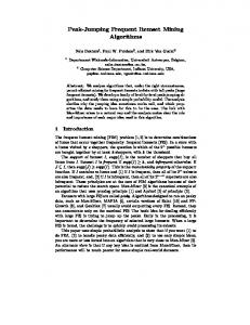
0.012 Real datasets: The four real datasets used in our len=180 Min_sup=0.005% len=160 Min_sup=0.004% experiments are connect, pumsb, mushroom, and gazelle, 0.01 len=140 Min_sup=0.003% 1 len=120 Min_sup=0.002% respectively. The connect dataset is a very dense len=100 Min_sup=0.001% 0.008 dataset, which contains game state information, the 0.1 0.006 pumsb dataset contains census data and is also a dense dataset, the mushroom dataset is a little (but not very) 0.004 0.01 dense and contains characteristics of various species of 0.002 mushrooms, while the gazelle dataset contains click0.001 0 stream data from Gazelle.com and is a very sparse 20 40 60 80 100 120 140 160 180 200 5 10 15 20 25 Length Length dataset with a few very long transactions. Synthetic datasets: The synthetic datasets were gen- Fig. 8. Support constraint Fig. 9. Support constraint (gazelle). (T10I4D100K ). erated from IBM dataset generator, and each contains totally 1000 distinct items with an average transaction length 10 and average frequent itemset length 4. The dataset T10I4D100K contains 100,000 transactions, while the dataset series T10I4Dx contain 200K 30%, 40%, and 50%, respectively, while Fig. 5 shows anto 1000K transactions, which were used to test the al- other four constraints with minimum support for itemsets longer than 25 set at 5%, 10%, 15%, and 20%, gorithm scalability. respectively. Fig. 6 shows another four special stairstyle length-decreasing support constraints for pumsb 100 70 Min_sup=50% Min_sup=20% dataset, with minimum support for itemsets longer Min_sup=40% Min_sup=15% 90 60 Min_sup=30% Min_sup=10% Min_sup=20% Min_sup=5% than 20 set at 40%, 50%, 60%, and 70%, respectively. 80 50 For dataset mushroom, we used a set of linear length70 40 decreasing support constraint functions: The support 60 30 threshold is set at 10% at length 1, and is linearly de50 20 creased to 0.01% at length 5, 10, 15, 20, respectively 40 10 30 (Because the y-axis in Fig. 7 is in log-scale, the cor20 0 responding curves do not look like linear functions, al5 10 15 20 25 30 5 10 15 20 25 30 though they are in fact linear. Similar situation hapLength Length Fig. 4. Support constraint Fig. 5. Support constraint pens in Fig. 8). For dataset gazelle, we chose five different support constraints: starting from support 1% (connect). (connect). for length 1, the support threshold will be linearly decreased to 0.04%, 0.02%, 0.01%, 0.005%, and 0.003% Length-decreasing support constraints: Fig. 4- at length 100, 120, 140, 160 and 180, respectively. Fig. 9 show various length-decreasing support constraints 9 shows a set of stair-style length-decreasing support used in our tests for different datasets. Fig. 4 and constraints chosen for dataset T10I4D100K, with miniFig. 5 depict two sets of stair-style length-decreasing mum support for length greater than 20 set at 0.001%, support constraints for dataset connect. Fig. 4 shows 0.002%, 0.003%, 0.004%, and 0.005%, respectively. four length-decreasing support constraints with minimum support for itemsets longer than 25 set at 20%, 4.2 Performance Testing

1e+08 # Constrained frequent patterns # Constrained frequent closed patterns

LPMiner BAMBOO 100 Runtime (in seconds)

Number of patterns

1e+07

1e+06

100000

10

10000 1 20

25

30 35 40 Minimum support (in %)

45

Fig. 10. frequent vs. closed(connect).

50

20

25

30 35 40 Minimum support (in %)

45

50

Fig. 11. Runtime comparison(connect).

Comparison with LPMiner We first compared BAMBOO with LPMiner in order to show that mining constrained closed itemsets is a more desirable task than mining constrained frequent itemsets. We used the datasets listed above and all showed the similar picture: BAMBOO can generate more concise result set while it is more efficient than LPMiner. Due to the limited space, here we only present the comparison results for the connect dataset. Fig. 10 compares the number of frequent itemsets with that of frequent closed itemsets, both satisfying the set of length-decreasing support constraints shown in Fig 4 (A minimum support 20% in Fig. 10 represents the length-decreasing support constraint whose minimum support is 20% for itemsets longer than 25). Fig. 11 shows the runtime of the two algorithms under the same set of length-decreasing support constraints. We can see BAMBOO generates orders of magnitude fewer patterns, and can be orders of magnitude faster than LPMiner. BAMBOO’s higher performance stems from two aspects: on the one hand, it mines much smaller number of valid itemsets than LPMiner, on the other hand, it adopts more effective pruning methods, which can make full use of the length-decreasing support constraint to prune the search space quickly. Comparison with CLOSET+ and CFP-tree We also compared BAMBOO with two recently developed frequent closed itemset mining algorithms, CFP-tree [15] and CLOSET+ [27]. In comparing these three algorithms, we recorded the total number of frequent closed itemsets and the number of closed itemsets which satisfy the corresponding length-decreasing support constraints shown in Fig 5-9 (We call it the number of constrained closed patterns in the corresponding figures). We first compared the three algorithms using the dataset connect and the support constraints shown in Fig. 5. From Fig. 13, we can see at high support threshold (e.g., 20%), BAMBOO can be several times faster than both CLOSET+ and CFP-tree, while at low support (e.g., 5%), BAMBOO can be several orders of

magnitude faster than CLOSET+ and CFP-tree. Fig. 12 shows that the length-decreasing support constraint is very effective in shrinking the result set, while on the other hand, it also implicates that as long as we can find some effective search space pruning methods for BAMBOO, it will be potentially more efficient than the traditional closed pattern mining algorithms. Fig. 14 and Fig. 15 show the comparison results for dataset pumsb: BAMBOO always generates much smaller number of patterns and runs much faster than CLOSET+ and CFP-tree under the length-decreasing support constraints shown in Fig. 6. For example, at support 50%, BAMBOO can be about 60 times faster than CLOSET+ and more than 100 times faster than CFP-tree, while the number of constrained closed patterns is about 30 times less than that of all frequent closed patterns. Unlike connect and pumsb, the mushroom dataset is relatively small and not very dense, from which a not too large number of frequent closed patterns can be found even with a very low support threshold like 0.01%. Even for such a small dataset, BAMBOO can still use some kind of length-decreasing support constraints to reduce the number of valid closed patterns and improve the performance. From Fig. 16 and Fig. 17, we know under the support constraints shown in Fig. 7, BAMBOO can be several times faster than CLOSET+ and CFP-tree, while its result set can be several times smaller. Gazelle is a very sparse dataset and can generate a few very long frequent closed itemsets with low support threshold. Most of the current closed itemset mining algorithms run too slow when the support threshold is lower than a certain threshold, this is because on the one hand mining long patterns itself is very challenging, on the other hand, a large number of short frequent closed patterns will be generated. Fig. 18 and Fig. 19 show very interesting and also amazing results: under the linearly length-decreasing support constraint functions shown in Fig. 8, BAMBOO can sift out most of the closed patterns and only a few very long itemsets with low support and a few short itemsets with high support are left. For example, if the support threshold is linearly decreased from 1% at length 1 to 0.003% at length 180, BAMBOO only finds 79 valid itemsets and the longest itemset has a length 184. Fig. 18 and Fig. 19 show that BAMBOO generates orders of magnitude fewer patterns and runs several orders of magnitude faster than CLOSET+ and CFP-tree. T10I4D100K is also a sparse dataset, from which a lot of short frequent closed itemsets can be mined for low support thresholds. Fig. 20 and Fig. 21 demonstrate the results for this dataset under the set of stair-style support constraints shown in Fig. 9.

1e+007

Runtime (in seconds)

Number of patterns

CFP-tree CLOSET+ BAMBOO

1e+06

Runtime (in seconds)

100000 10000 1000

10 100

1000

1000 100 10 1

110

120

130

140 150 Length

160

170

0.1 100

180

Fig. 18. constrained vs. non-constrained (gazelle).

100

CFP-tree CLOSET+ BAMBOO

10000

100

10000 # Frequent closed patterns # Constrained frequent closed patterns 1e+07

# Frequent closed patterns # Constrained frequent closed patterns

1e+006 Number of patterns

BAMBOO can be several times faster than CLOSET+, while can be several orders of magnitude faster than CFP-tree algorithm. In the meantime, the number of closed itemsets satisfying the length-decreasing support constraints is several times smaller than that of all frequent closed itemsets.

110

120

130

140 150 Length

160

170

180

Fig. 19. Runtime comparison(gazelle).

10 1e+07 # Frequent closed patterns # Constrained frequent closed patterns

1 8

10 12 14 16 Minimum support (in %)

18

20

6

Fig. 12. constrained vs. non-constrained(connect).

8

10 12 14 16 Minimum support (in %)

18

10000

20

Fig. 13. Runtime comparison(connect).

1e+06

Runtime (in seconds)

6

Number of patterns

100000

CFP-tree CLOSET+ BAMBOO

1000

100

10000 # Frequent closed patterns # Constrained frequent closed patterns

CFP-tree CLOSET+ BAMBOO Runtime (in seconds)

Number of patterns

1e+07

1e+06

100000

Fig. 20. constrained vs. non-constrained (T10I4D100K ).

1000

100

1000

1 40

45

50 55 60 Minimum support (in %)

65

70

40

Fig. 14. constrained vs. non-constrained(pumsb).

45

50 55 60 Minimum support (in %)

65

70

Fig. 15. Runtime comparison(pumsb).

25

300000 # Frequent closed patterns # Constrained frequent closed patterns

CFP-tree CLOSET+ BAMBOO Runtime (in seconds)

250000

200000

150000

100000 6

8

10

12 14 Length

16

18

20

Fig. 16. constrained vs. non-constrained (mushroom).

10 0.001 0.0015 0.002 0.0025 0.003 0.0035 0.004 0.0045 0.005 Minimum support (in %)

Fig. 21. Runtime comparison(T10I4D100K ).

10

10000

Number of patterns

0.001 0.0015 0.002 0.0025 0.003 0.0035 0.004 0.0045 0.005 Minimum support (in %)

20

15

10

5 6

8

10

12 14 Length

16

18

20

Fig. 17. Runtime comparison(mushroom).

Effectiveness of the pruning methods The above comparison results have validated the effectiveness of

the length-decreasing support constraints in compressing the result set: BAMBOO can generate orders of magnitude fewer patterns than the traditional all frequent closed pattern mining algorithms. But this does not mean any pattern discovery algorithms with lengthdecreasing support constraint will have much better performance than a frequent closed pattern mining algorithm. The efficiency of such kind of constrained algorithms mainly depends on whether we can propose some effective search space pruning methods. The above performance comparison results have to some extent already demonstrated the effectiveness of the pruning methods adopted by BAMBOO. Here we will use the T10I4D100K dataset to isolate the effectiveness of each pruning method used in BAMBOO. Fig. 22 shows the results under the support constraints in Fig. 9. The Legend “no-pruning” corresponds to the LPCLOSET algorithm, which does not apply any of the following three pruning methods, unpromising prefix itemset pruning, invalid item pruning 3 , and transaction prun3 Here

the unpromising prefix itemset pruning is the SVE enhanced version, while the invalid item pruning has been optimized using the binning technique.

pruning methods, unpromising prefix itemset pruning and invalid item pruning, plus some other optimization techniques have been newly proposed to enhance the performance. Our thorough performance study has shown that BAMBOO not only can generate orders of magnitude fewer patterns, but also can be orders of magnitude faster than both the recently developed frequent closed itemset mining algorithms and LPMiner, a frequent itemset mining algorithm with length decreasScalability test We also tested BAMBOO’s scalability ing support constraint. Furthermore, our experimenin terms of the base size by using the synthetic dataset tal study also testifies the effectiveness of the pruning series T10I4Dx. Here we varied the base size from 200K methods and good scalability of BAMBOO in terms of tuples to 1000K tuples and ran BAMBOO under the five number of transactions. different length-decreasing support constraints shown in Fig. 9. In presenting the results, we use a legend 6 Acknowledgments “S=0.001%” to represent the length-decreasing support We are grateful to Guimei Liu for providing us the constraint whose minimum support is 0.001% for length executable code of the CFP-tree algorithm. greater than 20. From Fig. 23, we know that BAMBOO has very good linear scalability against the number of References transactions in the dataset.

ing. We can see that compared to the LPCLOSET algorithm, each pruning method is very effective in boosting the performance and when we incorporate all the three pruning methods into BAMBOO, it achieves the best performance. In addition, in comparison to one of the best SVE-based pruning methods, transaction pruning, the pruning methods proposed in this paper, unpromising prefix itemset pruning and invalid item pruning, are more effective in enhancing the algorithm performance.

180

140 120 100 80 60

S=0.001% S=0.002% S=0.003% S=0.004% S=0.005%

120 Runtime (in seconds)

Runtime (in seconds)

160

No pruning transaction pruning Invalid item pruning Prefix itemset pruning BAMBOO

100 80 60 40

40 20 0.001 0.0015 0.002 0.0025 0.003 0.0035 0.004 0.0045 0.005 Minimum support (in %)

Fig. 22. Comparison of the pruning methods (T10I4D100K ).

20 200

300

400

500 600 700 800 Base szie (in K tuples)

900 1000

Fig. 23. Scalability test against base size(T10I4Dx ).

5 Conclusions Many previous studies have elaborated that mining frequent closed/maximal itemsets in large databases or mining frequent itemsets with length-decreasing support constraints can lead to more compact result set and possibly better performance. However, as our empirical study has showed these two kinds of algorithms still generate too many patterns when the support is low or the patterns become long. In this paper we developed BAMBOO, the first algorithm which can push deeply the length-decreasing support constraint into the traditional closed itemset mining in order to generate more concise and meaningful result set and gain better efficiency. Under this more general framework the downward-closure property no longer holds, we cannot use it to prune search space. Instead, two search space

[1] R. Agrawal, T. Imielinski, and A. Swami, Mining association rules between sets of items in large databases, ACM SIGMOD’93, May 1993. [2] R. Agrawal and R. Srikant, Fast algorithms for mining association rules, VLDB’94, Sept. 1994. [3] R.J. Bayardo, Efficiently Mining long patterns from databases, SIGMOD’98, June 1998. [4] S. Brin, R. Motwani, J.D. Ullman, S. Tsur, Dynamic Itemset Counting and Implication Rules for Market Basket Data, SIGMOD’97, May 1997. [5] C. Bucila, J. Gehrke, D. Kifer, W. White, DualMiner: a dual-pruning algorithm for itemsets with constraints, SIGKDD’02, July 2002. [6] D. Burdick, M. Calimlim, and J. Gehrke, MAFIA: A maximal frequent itemset algorithm for transactional databases, ICDE’01, April 2001. [7] E. Cohen, M. Datar, S. Fujiwara, A. Gionis, P. Indyk, R. Motwani, J.D. Ullman, C. Yang, Finding Interesting Associations without Support Pruning, ICDE’00, Feb. 2000. [8] M. El-Hajj, O. R. Za¨ıane, Inverted Matrix: Efficient Discovery of Frequent Items in Large Datasets in the Context of Interactive Mining, SIGKDD’03, Aug. 2003. [9] D. Gunopulos, H. Mannila, and S.Saluja, Discovering All Most Specific Sentences by Randomized Algorithms, ICDT’97, Jan. 1997. [10] R. J. Bayardo., R. Agrawal, D. Gunopulos, ConstraintBased Rule Mining in Large, Dense Databases, ICDE’99, Mar. 1999. [11] E. Han, G. Karypis, V. Kumar, Scalable Parallel Data Mining for Association Rules, SIGMOD’97, May 1997. [12] J. Han, J. Pei, Y. Yin, Mining frequent patterns without candidate generation, SIGMOD’00, May 2000. [13] J. Han, J. Wang, Y. Lu, and P. Tzvetkov, Mining Topk frequent closed patterns without minimum support, ICDM’02, Dec. 2002.

[14] B. Liu, W. Hsu, Y. Ma, Mining association rules with multiple minimum supports, SIGKDD’99, Aug. 1999. [15] G. Liu, H. Lu, W. Lou, J. X. Yu, On Computing, Storing and Querying Frequent Patterns, SIGKDD’03, Aug. 2003. [16] J. Liu, Y. Pan, K. Wang, and J. Han, Mining frequent item sets by opportunistic projection, SIGKDD’02, July 2002. [17] R.T. Ng, L.V.S. Lakshmanan, J. Han, and T. Mah, Exploratory mining via constrained frequent set queries, SIGMOD’99, June 1999. [18] F. Pan, G. Cong, A.K.H. Tung, J. Yang, M. Zaki, CARPENTER: Finding Closed Patterns in Long Biological Datasets, SIGKDDD’03, Aug. 2003. [19] J. Park, M. Chen, P.S. Yu, An Effective Hash Based Algorithm for Mining Association Rules, SIGMOD’95, May 1995. [20] N. Pasquier, Y. Bastide, R. Taouil, and L. Lakhal, Discovering frequent closed itemsets for association rules, ICDT’99, Jan. 1999. [21] Jian Pei, Jiawei Han, Can we push more constraints into frequent pattern mining? SIGKDD’00, Aug. 2000. [22] Jian Pei, Jiawei Han, Laks V. S. Lakshmanan, Mining Frequent Item Sets with Convertible Constraints, ICDE’01, April, 2001. [23] J. Pei, J. Han, H. Lu, S. Nishio, S. Tang, and D. Yang, H-Mine: Hyper-structure mining of frequent patterns in large databases, ICDM’01, Nov. 2001. [24] J. Pei, J. Han, and R. Mao, CLOSET: An efficient algorithm for mining frequent closed itemsets, DMKD’00, May 2000. [25] M. Seno, G. Karypis, LPMiner: An Algorithm for Finding Frequent Itemsets Using Length-Decreasing Support Constraint, ICDM’01, Nov. 2001. [26] H. Toivonen, Sampling Large Databases for Association Rules, VLDB’96, Sept. 1996. [27] J. Wang, J. Han, and J. Pei, CLOSET+: Searching for the Best Strategies for Mining Frequent Closed Itemsets, SIGKDD’03, Aug. 2003. [28] K. Wang, Y. He, J. Han, Mining Frequent Itemsets Using Support Constraints, VLDB’00, Sept. 2000. [29] M. Zaki, Generating non-redundant association rules, SIGKDD’00, Aug. 2000. [30] M. Zaki and C. Hsiao, CHARM: An efficient algorithm for closed itemset mining, SDM’02, April 2002. [31] Z. Zheng, R. Kohavi, and L. Mason, Real world performance of association rule algorithms, SIGKDD’01, Aug. 2001.