BASICS OF MECHANICAL ENGINEERING:

BASICS OF MECHANICAL ENGINEERING: INTEGRATING SCIENCE, TECHNOLOGY AND COMMON SENSE

Paul D. Ronney Department of Aerospace and Mechanical Engineering University of Southern California Available on-line at http://ronney.usc.edu/ame101/ Copyright © 2005 - 2017 by Paul D. Ronney. All rights reserved.

Table of contents TABLE OF CONTENTS

II

FOREWORD

IV

NOMENCLATURE

VII

CHAPTER 1. WHAT IS MECHANICAL ENGINEERING?

1

CHAPTER 2. UNITS

4

CHAPTER 3. “ENGINEERING SCRUTINY” Scrutinizing analytical formulas and results Scrutinizing computer solutions Examples of the use of units and scrutiny

10 10 12 13

CHAPTER 4. FORCES IN STRUCTURES Forces Degrees of freedom Moments of forces Types of forces and moments of force Analysis of statics problems

19 19 19 21 23 26

CHAPTER 5. STRESSES, STRAINS AND MATERIAL PROPERTIES Stresses and strains Pressure vessels Bending of beams Buckling of columns

35 35 45 47 54

CHAPTER 6. FLUID MECHANICS Fluid statics Equations of fluid motion

56 56 58 58 59 61 61 61 62 63 64 65 65 65 69 72

Bernoulli’s equation Conservation of mass

Viscous effects Definition of viscosity No-slip boundary condition Reynolds number Navier-Stokes equations Laminar and turbulent flow

Lift, drag and fluid resistance Lift and drag coefficients Flow around spheres and cylinders Flow through pipes

Compressible flow CHAPTER 7. THERMAL AND ENERGY SYSTEMS ii

76

Conservation of energy – First Law of Thermodynamics Statement of the First Law Describing a thermodynamic system Conservation of energy for a control mass or control volume Processes Examples of energy analysis using the 1st Law

Second Law of thermodynamics Engines cycles and efficiency Heat transfer Conduction Convection Radiation

CHAPTER 8. WRITTEN AND ORAL COMMUNICATION APPENDIX A. DESIGN PROJECTS Generic information about the design projects How to run a meeting (PDR’s philosophy…) Suggestions for the written report

King of the Hill Spaghetti Bridge Candle-powered boat Plaster of Paris Bridge Hydro power

76 76 79 79 81 81 85 86 90 91 92 93 94 100 100 100 100 103 107 111 113 116

APPENDIX B. PROBLEM-SOLVING METHODOLOGY

120

APPENDIX C. EXCEL TUTORIAL

121

APPENDIX D. STATISTICS Mean and standard deviation Stability of statistics Least-squares fit to a set of data

124 124 125 126

iii

Foreword If you’re reading this book, you’re probably already enrolled in an introductory university course in Mechanical Engineering. The primary goals of this textbook are, to provide you, the student, with: 1. An understanding of what Mechanical Engineering is and to a lesser extent what it is not 2. Some useful tools that will stay with you throughout your engineering education and career 3. A brief but significant introduction to the major topics of Mechanical Engineering and enough understanding of these topics so that you can relate them to each other 4. A sense of common sense The challenge is to accomplish these objectives without overwhelming you so much that you won’t be able to retain the most important concepts. In regards to item 2 above, I remember nothing about some of my university courses, even in cases where I still use the information I learned therein. In others I remember “factoids” that I still use. One goal of this textbook is to provide you with a set of useful factoids so that even if you don’t remember any specific words or figures from this text, and don’t even remember where you learned these factoids, you still retain them and apply them when appropriate. In regards to item 3 above, in particular the relationships between topics, this is one area where I feel engineering faculty (myself included) do not do a very good job. Time and again, I find that students learn something in class A, and this information is used with different terminology or in a different context in class B, but the students don’t realize they already know the material and can exploit that knowledge. As the old saying goes, “We get too soon old and too late smart…” Everyone says to themselves several times during their education, “oh… that’s so easy… why didn’t the book [or instructor] just say it that way…” I hope this text will help you to get smarter sooner and older later. A final and less tangible purpose of this text (item 4 above) is to try to instill you with a sense of common sense. Over my 29 years of teaching, I have found that students have become more technically skilled and well rounded but have less ability to think and figure out things for themselves. I attribute this in large part to the fact that when I was a teenager, cars were relatively simple and my friends and I spent hours working on them. When our cars weren’t broken, we would sabotage (nowadays “hack” might be a more descriptive term) each others’ cars. The best hacks were those that were difficult to diagnose, but trivial to fix once you figured out what was wrong. We learned a lot of common sense working on cars. Today, with electronic controls, cars are very difficult to work on or hack. Even with regards to electronics, today the usual solution to a broken device is to throw it away and buy a newer device, since the old one is probably nearly obsolete by the time it breaks. Of course, common sense per se is probably not teachable, but a sense of common sense, that is, to know when it is needed and how to apply it, might be teachable. If I may be allowed an immodest moment in this textbook, I would like to give an anecdote about my son Peter. When he was not quite 3 years old, like most kids his age had a pair of shoes with lights (actually light-emitting diodes or LEDs) that flash as you walk. These shoes work for a few months until the heel switch fails (usually in the closed position) so that the LEDs stay on continuously for a day or two until the battery goes dead. One morning he noticed that the LEDs in one of his shoes were on continuously. He had a puzzled look on his face, but said nothing. Instead, he went to look for his other shoe, and after rooting around a bit, found it. He then picked it up, hit it against iv

something and the LEDs flashed as they were supposed to. He then said, holding up the good shoe, “this shoe - fixed… [then pointing at the other shoe] that shoe - broken!” I immediately thought, “I wish all my students had that much common sense…” In my personal experience, about half of engineering is common sense as opposed to specific, technical knowledge that needs to be learned from coursework. Thus, to the extent that common sense can be taught, a final goal of this text is to try to instill this sense of when common sense is needed and even more importantly how to integrate it with technical knowledge. The most employable and promotable engineering graduates are the most flexible ones, i.e. those that take the attitude, “I think I can handle that” rather than “I can’t handle that since no one taught me that specific knowledge.” Students will find at some point in their career, and probably in their very first job, that plans and needs change rapidly due to testing failures, new demands from the customer, other engineers leaving the company, etc. In most engineering programs, retention of incoming first-year students is an important issue; at many universities, less than half of first-year engineering students finish an engineering degree. Of course, not every incoming student who chooses engineering as his/her major should stay in engineering, nor should every student who lacks confidence in the subject drop out, but in all cases it is important that incoming students receive a good enough introduction to the subject that they make an informed, intelligent choice about whether he/she should continue in engineering. Along the thread of retention, I would like to give an anecdote. At Princeton University, in one of my first years of teaching, a student in my thermodynamics class came to my office, almost in tears, after the first midterm. She did fairly poorly on the exam, and she asked me if I thought she belonged in Engineering. (At Princeton thermodynamics was one of the first engineering courses that students took). What was particularly distressing to her was that her fellow students had a much easier time learning the material than she did. She came from a family of artists, musicians and dancers and got little support or encouragement from home for her engineering studies. While she had some of the artistic side in her blood, she said that her real love was engineering, but she wondered was it a lost cause for her? I told her that I didn’t really know whether she should be an engineer, but I would do my best to make sure that she had a good enough experience in engineering that she could make an informed choice from a comfortable position, rather than a decision made under the cloud of fear of failure. With only a little encouragement from me, she did better and better on each subsequent exam and wound up receiving a very respectable grade in the class. She went on to graduate from Princeton with honors and earn a Ph.D. in engineering from a major Midwestern university. I still consider her one of my most important successes in teaching. Thus, a goal of this text is (along with the instructor, teaching assistants, fellow students, and infrastructure) is to provide a positive first experience in engineering. There are also many topics that should be (and in some instructors’ views, must be) covered in an introductory engineering textbook but are not covered here because the overriding desire to keep the book’s material manageable within the limits of a one-semester course: 1. 2. 3.

History of engineering Philosophy of engineering Engineering ethics

Finally, I offer a few suggestions for faculty using this book: 1. 2.

Projects. I assign small, hands-on design projects for the students, examples of which are given in Appendix A. Demonstrations. Include simple demonstrations of engineering systems – thermoelectrics, piston-type internal combustion engines, gas turbine engines, transmissions, … v

3.

Computer graphics. At USC, the introductory Mechanical Engineering course is taught in conjunction with a computer graphics laboratory where an industry-standard software package is used.

vi

Nomenclature Symbol A BTU CD CL CP CV c COP d E E e F f g gc h I I k k L M M M m m n NA P P Q q  R R Re r S T T

Meaning Area British Thermal Unit Drag coefficient Lift coefficient Specific heat at constant pressure Specific heat at constant volume Sound speed Coefficient Of Performance Diameter Energy Elastic modulus Internal energy per unit mass Force Friction factor (for pipe flow) Acceleration of gravity USCS units conversion factor Convective heat transfer coefficient Area moment of inertia Electric current Boltzmann’s constant Thermal conductivity Length Molecular Mass

SI units and/or value m2 1 BTU = 1055 J ----J/kgK J/kgK m/s --m (meters) J (Joules) N/m2 J/kg N (Newtons) --m/s2 (earth gravity = 9.81) 32.174 lbm ft/ lbf sec2 = 1 W/m2K m4 amps 1.380622 x 10-23 J/K W/mK m kg/mole

Moment of force Mach number Mass Mass flow rate Number of moles Avogadro’s number (6.0221415 x 1023) Pressure Point-load force Heat transfer Heat transfer rate Universal gas constant Mass-based gas constant = Â/M Electrical resistance Reynolds number Radius Entropy Temperature Tension (in a rope or cable)

N m (Newtons x meters) --kg kg/s ----N/m2 N J W (Watts) 8.314 J/mole K J/kg K ohms --m J/K K N

t U u V V V v W W w Z z

Time Internal energy Internal energy per unit mass Volume Voltage Shear force Velocity Weight Work Loading (e.g. on a beam) Thermoelectric figure of merit elevation

s (seconds) J J/kg m3 Volts N m/s N (Newtons) J N/m 1/K m

a g h e e µ µ q n n r r s s s t t

Thermal diffusivity Gas specific heat ratio Efficiency Strain Roughness factor (for pipe flow) Coefficient of friction Dynamic viscosity Angle Kinematic viscosity = µ/r Poisson’s ratio Density Electrical resistivity Normal stress Stefan-Boltzmann constant Standard deviation Shear stress Thickness (e.g. of a pipe wall)

m2/s ----------kg/m s --m2/s --kg/m3 ohm m N/m2 5.67 x 10-8 W/m2K4 [Same units as sample set] N/m2 m

---

viii

Chapter 1. What is Mechanical Engineering? “The journal of a thousand miles begins with one step.” - Lao Zhu Definition of Mechanical Engineering My personal definition of Mechanical Engineering is If it needs engineering but it doesn’t involve electrons, chemical reactions, arrangement of molecules, life forms, isn’t a structure (building/bridge/dam) and doesn’t fly, a mechanical engineer will take care of it… but if it does involve electrons, chemical reactions, arrangement of molecules, life forms, is a structure or does fly, mechanical engineers may handle it anyway Although every engineering faculty member in every engineering department will claim that his/her field is the broadest engineering discipline, in the case of Mechanical Engineering that’s actually true (I claim) because the core material permeates all engineering systems (fluid mechanics, solid mechanics, heat transfer, control systems, etc.) Mechanical engineering is one of the oldest engineering fields (though perhaps Civil Engineering is even older) but in the past 20 years has undergone a rather remarkable transformation as a result of a number of new technological developments including •

• •

•

•

Computer Aided Design (CAD). The average non-technical person probably thinks that mechanical engineers sit in front of a drafting table drawing blueprints for devices having nuts, bolts, shafts, gears, bearings, levers, etc. While that image was somewhat true 100 years ago, today the drafting board has long since been replaced by CAD software, which enables a part to be constructed and tested virtually before any physical object is manufactured. Simulation. CAD allows not only sizing and checking for fit and interferences, but the resulting virtual parts are tested structurally, thermally, electrically, aerodynamically, etc. and modified as necessary before committing to manufacturing. Sensor and actuators. Nowadays even common consumer products such as automobiles have dozens of sensors to measure temperatures, pressures, flow rates, linear and rotational speeds, etc. These sensors are used not only to monitor the health and performance of the device, but also as inputs to a microcontroller. The microcontroller in turn commands actuators that adjust flow rates (e.g. of fuel into an engine), timings (e.g. of spark ignition), positions (e.g. of valves), etc. 3D printing. Traditional “subtractive manufacturing” consisted of starting with a block or casting of material and removing material by drilling, milling, grinding, etc. The shapes that can be created in this way are limited compared to modern “additive manufacturing” or “3D printing” in which a structure is built in layers. Just as CAD + simulation has led to a new way of designing systems, 3D printing has led to a new way of creating prototypes and in limited cases, full-scale production. Collaboration with other fields. Historically, a nuts-and-bolts device such as an automobile was designed almost exclusively by mechanical engineers. Modern vehicles have vast electrical and electronic systems, safety systems (e.g. air bags, seat restraints), specialized batteries (in the

case of hybrids or electric vehicles), etc., which require design contributions from electrical, biomechanical and chemical engineers, respectively. It is essential that a modern mechanical engineer be able to understand and accommodate the requirements imposed on the system by non-mechanical considerations. These radical changes in what mechanical engineers do compared to a relatively short time ago makes the field both challenging and exciting. Mechanical Engineering curriculum In almost any accredited Mechanical Engineering program, the following courses are required: • • • • • • •

•

Basic sciences - math, chemistry, physics Breadth or distribution (called “General Education” at USC) Computer graphics and computer aided design (CAD) Experimental engineering & instrumentation Mechanical design - nuts, bolts, gears, welds Computational methods - converting continuous mathematical equations into discrete equations solved by a computer Core “engineering science” o Dynamics – essentially F = ma applied to many types of systems o Strength and properties of materials o Fluid mechanics o Thermodynamics o Heat transfer o Control systems Senior “capstone” design project

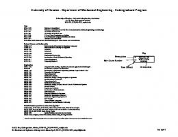
Additionally you may participate in non-credit “enrichment” activities such as undergraduate research, undergraduate student paper competitions in ASME (American Society of Mechanical Engineers, the primary professional society for mechanical engineers), the SAE Formula racecar project, etc.

Figure 1. SAE Formula racecar project at USC (photo: http://www.uscformulasae.com) 2

Examples of industries employing MEs Many industries employ mechanical engineers; a few industries and the type of systems MEs design are listed below. o Automotive • Combustion • Engines, transmissions • Suspensions o Aerospace (w/ aerospace engineers) • Control systems • Heat transfer in turbines • Fluid mechanics (internal & external) o Biomedical (w/ physicians) • Biomechanics – prosthesis • Flow and transport in vivo o Computers (w/ computer engineers) • Heat transfer • Packaging of components & systems o Construction (w/ civil engineers) • Heating, ventilation, air conditioning (HVAC) • Stress analysis o Electrical power generation (w/ electrical engineers) • Steam power cycles - heat and work • Mechanical design of turbines, generators, ... o Petrochemicals (w/ chemical, petroleum engineers) • Oil drilling - stress, fluid flow, structures • Design of refineries - piping, pressure vessels o Robotics (w/ electrical engineers) • Mechanical design of actuators, sensors • Stress analysis

3

Chapter 2. Units I often say that when you can measure what you are speaking about, and express it in numbers, you know something about it; but when you cannot measure it, when you cannot express it in numbers, your knowledge is of a meagre and unsatisfactory kind; it may be the beginning of knowledge, but you have scarcely, in your thoughts, advanced to the stage of science, whatever the matter may be – William Thompson (Lord Kelvin) All engineered systems require measurements for specifying the size, weight, speed, etc. of objects as well as characterizing their performance. Understanding the application of these units is the single most important objective of this textbook because it applies to all forms of engineering and everything that one does as an engineer. Understanding units is far more than simply being able to convert from feet to meters or vice versa; combining and converting units from different sources is a challenging topic. For example, if building insulation is specified in units of BTU inches per hour per square foot per degree Fahrenheit, how can that be converted to thermal conductivity in units of Watts per meter per degree C? Or can it be converted? Are the two units measuring the same thing or not? (For example, in a new engine laboratory facility that was being built for me, the natural gas flow was insufficient… so I told the contractor I needed a system capable of supplying a minimum of 50 cubic feet per minute (cfm) of natural gas at 5 pounds per square inch (psi). His response was “what’s the conversion between cfm and psi?” Of course, the answer is that there is no conversion; cfm is a measure of flow rate and psi a measure of pressure.) Engineers must struggle with these misconceptions every day. Engineers in the United States are burdened with two systems of units and measurements: (1) the English or USCS (US Customary System) L and (2) the metric or SI (Système International d’Unités) J. Either system has a set of base units , that is, units which are defined based on a standard measure such as a certain number of wavelengths of a particular light source. These base units include: •

• • •

Length (meters (m), centimeters (cm), millimeters (mm); feet (ft), inches (in), kilometers (km), miles (mi)) • 1 m = 100 cm = 1000 mm = 3.281 ft = 39.37 in • 1 km = 1000 m • 1 mi = 5280 ft Mass (lbm, slugs, kilograms); (1 kg = 2.205 lbm = 0.06853 slug) (lbm = “pounds mass”) Time (seconds; the standard abbreviation is “s” not “sec”) (same units in USCS and SI!) Electric current (really electric charge in units of coulombs [abbreviation: ‘coul’] is the base unit and the derived unit is current = charge/time) (1 coulomb = charge on 6.241506 x 1018 electrons) (1 ampere [abbreviation: amp]= 1 coul/s)

Moles are often reported as a fundamental unit, but it is not; it is just a bookkeeping convenience to avoid carrying around factors of 1023 everywhere. The choice of the number of particles in a mole of particles is completely arbitrary; by convention Avogadro’s number is defined by NA = 6.0221415 x 1023, the units being particles/mole (or one could say individuals of any kind, not limited just to particles, e.g. atoms, molecules, electrons or students).

4

Temperature is frequently interpreted as a base unit but again it is not, it is a derived unit, that is, one created from combinations of base units. Temperature is essentially a unit of energy divided by Boltzman’s constant. Specifically, the average kinetic energy of an ideal gas particle in a 3dimensional box is 1.5kT, where k is Boltzman’s constant = 1.380622 x 10-23 J/K (really (Joules/particle)/K; every textbook will state the units as just J/K but you’ll see below how useful it is to include the “per particle” part as well). Thus, 1 Kelvin is the temperature at which the kinetic energy of an ideal gas (and only an ideal gas, not any other material) molecule is 1.5kT =2.0709 x 10-23 J. The ideal gas constant (Â) with which are you are very familiar is simply Boltzman’s constant multiplied by Avogadro’s number, i.e. ⎛ ⎞⎛ ⎞ J J cal 23 particle ℜ = kN A = ⎜1.38 ×10−23 = 1.987 ⎟⎜ 6.02 ×10 ⎟ = 8.314 particle K ⎠⎝ mole ⎠ mole K mole K ⎝

In the above equation, note that we have multiplied and divided units such as Joules as if they were numbers; this is valid because we can think of 8.314 Joules as 8.314 x (1 Joule) and additionally we can write (1 Joule) / (1 Joule) = 1. Extending that further, we can think of (1 Joule) / (1 kg m2/s2) = 1, which will be the basis of our approach to units conversion – multiplying and dividing by 1 written in different forms. There’s also another type of gas constant R = Â/M, where M = molecular mass of the gas; R depends on the type of gas whereas  is the “universal” gas constant, i.e., the same for any gas. Why does this discussion apply only for an ideal gas? By definition, ideal gas particles have only kinetic energy and negligible potential energy due to inter-molecular attraction; if there is potential energy, then we need to consider the total internal energy of the material (E, units of Joules) which is the sum of the microscopic kinetic and potential energies, in which case the temperature for any material (ideal gas or not) is defined as

# ∂U & T ≡% ( $ ∂S 'V =const.

(Equation 1)

where S is the entropy of the material (units J/K) and V is the volume. This intimidating-looking definition of temperature, while critical to understanding thermodynamics, will not be needed in this course. Derived units are units created from combinations of base units; there are an infinite number of possible derived units. Some of the more important/common/useful ones are: • • • • •

Area = length2; 640 acres = 1 mile2, or 1 acre = 43,560 ft2 Volume = length3; 1 ft3 = 7.481 gallons = 28,317 cm3; also 1 liter = 1000 cm3 = 61.02 in3 Velocity = length/time Acceleration = velocity/time = length/time2 (standard gravitational acceleration on earth = g = 32.174 ft/s2 = 9.806 m/s2) Force = mass * acceleration = mass*length/time2 o 1 kg m/s2 = 1 Newton = 0.2248 pounds force (pounds force is usually abbreviated lbf and Newton N) (equivalently 1 lbf = 4.448 N) 5

•

• • • • • • • • • •

Energy = force x length = mass x length2/time2 o 1 kg m2/s2 = 1 Joule (J) o 778 ft lbf = 1 British thermal unit (BTU) o 1055 J = 1 BTU o 1 J = 0.7376 ft lbf o 1 calorie = 4.184 J o 1 dietary calorie = 1000 calories Power (energy/time = mass x length2/time3) o 1 kg m2/s3 = 1 Watt o 746 W = 550 ft lbf/sec = 1 horsepower Heat capacity = J/moleK or J/kgK or J/mole˚C or J/kg˚C (see note below) Pressure = force/area o 1 N/m2 = 1 Pascal o 101325 Pascal = 101325 N/m2 = 14.686 lbf/in2 = 1 standard atmosphere Current = charge/time (1 amp = 1 coulomb/s) Voltage = energy/charge (1 Volt = 1 J/coulomb) Capacitance = amps / (volts/s) (1 farad = 1 coul2/J) Inductance = volts / (amps/s) (1 Henry = 1 J s2 / coul2) Resistance = volts/amps (1 ohm = 1 volt/amp = 1 Joule-s / coul2) Torque = force x lever arm length = mass x length2/time2 – same as energy but one would usually report torque in Nm (Newton meters), not Joules, to avoid confusion. Radians, degrees, revolutions – these are all dimensionless quantities, but must be converted between each other, i.e. 1 revolution = 2π radians = 360 degrees.

By far the biggest problem with USCS units is with mass and force. The problem is that pounds is both a unit of mass AND force. These are distinguished by lbm for pounds (mass) and lbf for pounds (force). We all know that W = mg where W = weight, m = mass, g = acceleration of gravity. So 1 lbf = 1 lbm x g = 32.174 lbm ft/s2

(Equation 2)

Sounds ok, huh? But wait, now we have an extra factor of 32.174 floating around. Is it also true that 1 lbf = 1 lbm ft/s2 which is analogous to the SI unit statement that 1 Newton = 1 kg m/s2

(Equation 3)

No, 1 lbf cannot equal 1 lbm ft/s2 because 1 lbf equals 32.174 lbm ft/sec2. So what unit of mass satisfies the relation 1 lbf = 1 (mass unit) ft/s2? This mass unit is called a “slug” believe it or not. With use of equation (2) it is apparent that 1 slug = 32.174 lbm = 14.59 kg

(Equation 4)

6

Often when doing USCS conversions, it is convenient to introduce a conversion factor called gc; by rearranging Equation 2 we can write gc =

32.174 lbm ft =1 lbf s2

(Equation 5).

Since Equation 2 shows that gc = 1, one can multiply and divide any equation by gc as many times as necessary to get the units into a more compact form (an example of “why didn’t somebody just say that?”). Keep in mind that any units conversion is simply a matter of multiplying or dividing by 1, e.g.

5280 ft 1 kg m 778 ft lbf = 1; = 1; = 1; etc. 2 mile BTU Ns For some reason 32.174 lbm ft/ lbf s2 has been assigned a special symbol called gc even though there are many other ways of writing 1 (e.g. 5280 ft / mile, 1 kg m / N s2, 778 ft lbf / BTU) all of which are also equal to 1 but none of which are assigned special symbols. If this seems confusing, I don’t blame you. That’s why I recommend that even for problems in which the givens are in USCS units and where the answer is needed in USCS units, first convert everything to SI units, do the problem, then convert back to USCS units. I disagree with some authors who say an engineer should be fluent in both systems; it is somewhat useful but not necessary. The first example below uses the approach of converting to SI, do the problem, and convert back to USCS. The second example shows the use of USCS units employing gc: Example 1 What is the weight (in lbf) of one gallon of air at 1 atm and 25˚C? The molecular mass of air is 28.97 g/mole = 0.02897 kg/mole. Ideal gas law: PV = nÂT (P = pressure, V = volume, n = number of moles, Â = universal gas constant, T = temperature) Mass of gas (m) = moles x mass/mole = nM (M = molecular mass) Weight of gas (W) = mg Combining these 3 relations: W = PVMg/ÂT

7

3 " 101325N/m 2 %" ft 3 " m % %" 0.02897kg %" 9.81m % $ '$ 1atm 1gal $ ' '$ ' $ '$ atm 7.481gal # 3.281ft & '&# mole &# s2 & &# PV Mg # W= = 8.314J ℜT (25+273)K moleK " N % 3 " kg %" m % "m% " m% N ) ( m ) ( kg) $ 2 ' Nm ) $ kg 2 ' $ 2 '(m ) $ '$ 2 ' ( ( #m & # mole &# s & #s & # s & = 0.0440 = 0.0440 = 0.0440 J J J mole 0.2248 lbf = 0.0440 N = 0.00989 lbf ≈ 0.01 lbf N

Note that it’s easy to write down all the formulas and conversions. The tricky part is to check to see if you’ve actually gotten all the units right. In this case I converted everything to the SI system first, then converted back to USCS units at the very end – which is a pretty good strategy for most problems. The tricky parts are realizing (1) the temperature must be an absolute temperature, i.e. Kelvin not ˚C, and (2) the difference between the universal gas constant  and the mass-specific constant R = Â/M. If in doubt, how do you know which one to use? Check the units! Example 2 A 3000 pound (3000 lbm) car is moving at a velocity of 88 ft/sec. What is its kinetic energy (KE) in units of ft lbf? What is its kinetic energy in Joules? 2

KE =

2 ! ft $ 1 1 2 7 lbm ft mass velocity = 3000 lbm 88 = 1.16 ×10 & ( )( ) ( ) #" 2 2 s% s2

Now what can we do with lbm ft2/sec2??? The units are (mass)(length)2/(time)2, so it is a unit of energy, so at least that part is correct. Dividing by gc, we obtain

KE = 1.16 ×107

2 ⎞⎛ ⎞ lbm ft 2 1 ⎛ lbf s 2 7 lbm ft × = 1.16 ×10 ⎜ ⎟ ⎜ ⎟ = 3.61×105 ft lbf gc ⎝ s2 s 2 ⎠⎝ 32.174 lbm ft ⎠

# & 1J 5 KE = ( 3.61×10 5 ft lbf )% ( = 4.89 ×10 J $ 0.7376 ft lbf '

Note that if you used 3000 lbf rather than 3000 lbm in the expression for KE, you’d have the wrong units – ft lbf2/lbm, which is NOT a unit of energy (or anything else that I know of…) Also note € that since gc = 1, we COULD multiply by gc rather than divide by gc; the resulting units (lbm2 ft3 /lbf sec4) is still a unit of energy, but not a very useful one! Many difficulties also arise with units of temperature. There are four temperature scales in “common” use: Fahrenheit, Rankine, Celsius (or Centigrade) and Kelvin. Note that one speaks of

8

“degrees Fahrenheit” and “degrees Celsius” but just “Rankines” or “Kelvins” (without the “degrees”). T (in units of ˚F) = T (in units of R) - 459.67 T (in units of ˚C) = T (in units of K) - 273.15 1 K = 1.8 R T (in units of˚C) = [T (in units of ˚F) – 32]/1.8, T (in units of ˚F) = 1.8[T (in units of ˚C)] + 32 Water freezes at 32˚F / 0˚C, boils at 212˚F / 100˚C Special note (another example of “that’s so easy, why didn’t somebody just say that?”): when using units involving temperature (such as heat capacity, units J/kg˚C, or thermal conductivity, units Watts/m˚C), one can convert the temperature in these quantities these to/from USCS units (e.g. heat capacity in BTU/lbm˚F or thermal conductivity in BTU/hr ft ˚F) simply by multiplying or dividing by 1.8. You don’t need to add or subtract 32. Why? Because these quantities are really derivatives with respect to temperature (heat capacity is the derivative of internal energy with respect to temperature) or refer to a temperature gradient (thermal conductivity is the rate of heat transfer per unit area by conduction divided by the temperature gradient, dT/dx). When one takes the derivative of the constant 32, you get zero. For example, if the temperature changes from 84˚C to 17˚C over a distance of 0.5 meter, the temperature gradient is (84-17)/0.5 = 134˚C/m. In Fahrenheit, the gradient is [(1.8*84 +32) – (1.8*17 + 32)]/0.5 = 241.2˚F/m or 241.2/3.281 = 73.5˚F/ft. The important point is that the 32 cancels out when taking the difference. So for the purpose of converting between ˚F and ˚C in units like heat capacity and thermal conductivity, one can use 1˚C = 1.8˚F. That doesn’t mean that one can just skip the + or – 32 whenever one is lazy. Also, one often sees thermal conductivity in units of W/m˚C or W/mK. How does one convert between the two? Do you have to add or subtract 273? And how do you add or subtract 273 when the units of thermal conductivity are not degrees? Again, thermal conductivity is heat transfer per unit area per unit temperature gradient. This gradient could be expressed in the above example as (84˚C-17˚C)/0.5 m = 134˚C/m, or in Kelvin units, [(84 + 273)K – (17 + 273)K]/0.5 m = 134K/m and thus the 273 cancels out. So one can say that 1 W/m˚C = 1 W/mK, or 1 J/kg˚C = 1 J/kgK. And again, that doesn’t mean that one can just skip the + or – 273 (or 460, in USCS units) whenever one is lazy.

Example 3 inch The thermal conductivity of a particular brand of ceramic insulating material is 0.5 BTU 2

ft hour °F

(I’m not kidding, these are the units commonly reported in commercial products!) What is the thermal conductivity in units of Watts ? meter °C

0.5

BTU inch 1055 J ft 3.281 ft hour 1 Watt 1.8˚F Watt × × × × × × = 0.0721 2 ft hour °F BTU 12 inch m 3600 s 1 J/s ˚C m˚C

Note that the thermal conductivity of air at room temperature is 0.026 Watt/m˚C, i.e. about 3 times lower than the insulation. So why don’t we use air as an insulator? We’ll discuss that in Chapter 7.

9

Chapter 3. “Engineering scrutiny” “Be your own worst critic, unless you prefer that someone else be your worst critic.” - I dunno, I just made it up. But, it doesn’t sound very original.

Scrutinizing analytical formulas and results I often see analyses that I can tell within 5 seconds must be wrong. I have three tests, which should be done in the order listed, for checking and verifying results. These tests will weed out 95% of all mistakes. I call these the “smoke test,” “function test,” and “performance test,” by analogy with building electronic devices. 1. Smoke test. In electronics, this corresponds to turning the power switch on and seeing if the device smokes or not. If it smokes, you know the device can’t possibly be working right (unless you intended for it to smoke.) In analytical engineering terms, this corresponds to checking the units. You have no idea how many results people report that can’t be correct because the units are wrong (i.e. the result was 6 kilograms, but they were trying to calculate the speed of something.) You will catch 90% of your mistakes if you just check the units. For example, if I just derived the ideal gas law for the first time and predicted PV = nÂ/T you can quickly see that the units on the right-hand side of the equation are different from those on the left-hand side. There are several additional rules that must be followed: •

Anything inside a square root, cube root, etc. must have units that are a perfect square (e.g. m2/sec2), cube, etc.) This does not mean that every term inside the square root must be a perfect square, only that the combination of all terms must be a perfect square. For example, the speed (v) of a frictionless freely falling object in a gravitational field is

v = 2gh , where g = acceleration of gravity (units length/time2) and h is the height from which the object was dropped (units length). Neither g nor h have units that are a perfect square, but when multiplied together the units are (length/time2)(length) = length2/time2, which is a perfect square, and when you take the square root, the units are

v = length 2 time 2 = length time as required. • •

Anything inside a log, exponent, trigonometric function, etc., must be dimensionless (I don’t know how to take the log of 6 kilograms). Again, the individual terms inside the function need not all be dimensionless, but the combination must be dimensionless. Any two quantities that are added together must have the same units (I can’t add 6 kilograms and 19 meters/second. Also, I can add 6 miles per hour and 19 meters per second, but I have to convert 6 miles per hour into meters per second, or convert 19 meters per second into miles per hour, before adding the terms together.)

2. Function test. In electronics, this corresponds to checking to see if the device does what I designed it to do, e.g. that the red light blinks when I flip switch on, the meter reading increases when I turn the knob to the right, the bell rings when I push the button, etc. – assuming that was what I intended that it do. In analytical terms this corresponds to determining if the result gives sensible predictions. Again, there are several rules that must be followed:

10

• • •

•

Determine if the sign (+ or -) of the result is reasonable. For example, if your prediction of the absolute temperature of something is –72 Kelvin, you should check your analysis again. For terms in an equation with property values in the denominator, can that value be zero? (In which case the term would go to infinity). Even if the property can’t go to zero, does it make sense that as the value decreases, the term would increase? Determine whether what happens to y as x goes up or down is reasonable or not. For example, in the ideal gas law, PV = nÂT: o At fixed volume (V) and number of moles of gas (n), as T increases then P increases – reasonable o At fixed temperature (T) and n, as V increases then P decreases – reasonable o Etc. Determine what happens in the limit where x goes to special values, e.g. zero, one or infinity as appropriate. For example, consider the equation for the temperature as a function of time T(t) of an object starting at temperature Ti at time t = 0 having surface area A (units m2), volume V (units m3), density r (units kg/m3) and heat capacity CP (units J/kg˚C) that is suddenly dunked into a fluid at temperature T∞ with heat transfer coefficient h (units Watts/m2˚C). It can be shown that in this case T(t) is given by

% hA ( T(t) = T∞ + (Ti − T∞ )exp' − t* & ρVCP )

€

•

(Equation 6)

hA/rVCP has units of (Watts/m2˚C)(m2)/(kg/m3)(m3)(J/kg˚C) = 1/s, so (hA/rVCP)t is dimensionless, thus the formula easily passes the smoke test. But does it make sense? At t = 0, Ti = 0 as expected. What happens if you wait for a long time? The temperature can reach T∞ but cannot overshoot it (a consequence of the Second Law of Thermodynamics, discussed in Chapter 7). In the limit t ® ∞, the term exp(-(hA/rVCP)t) goes to zero, thus T ® T∞ as expected. Other scrutiny checks: if h or A increases, heat can be transferred to the object more quickly, thus the time to approach T∞ decreases. Also, if r, V or CP increases, the “thermal inertia” (resistance to change in temperature) increases, so the time required to approach T∞ increases. So, the formula makes sense. If your formula contains a difference of terms, determine what happens if those 2 terms are equal. For example, in the above formula, if Ti = T∞, then the formula becomes simply T(t) = T∞ for all time. This makes sense because if the bar temperature and fluid temperature are the same, then there is no heat transfer to or from the bar and thus its temperature never changes (again, a consequence of the Second Law of Thermodynamics … two objects at the same temperature cannot exchange energy via heat transfer.)

3. Performance test. In electronics, this corresponds to determining how fast, how accurate, etc. the device is. In analytical terms this corresponds to determining how accurate the result is. This means of course you have to compare it to something else that you trust, i.e. an experiment, a more sophisticated analysis, someone else’s published result (of course there is no guarantee that their result is correct just because it got published, but you need to check it anyway.) For example, if I derived the ideal gas law and predicted PV = 7nRT, it passes the smoke and function tests with no problem, but it fails the performance test miserably (by a factor of 7). But

11

of course the problem is deciding which result to trust as being at least as accurate as your own result; this of course is something that cannot be determined in a rigorous way, it requires a judgment call based on your experience.

Scrutinizing computer solutions (This part is beyond what I expect you to know for AME 101 but I include it for completeness). Similar to analyses, I often see computational results that I can tell within 5 seconds must be wrong. It is notoriously easy to be lulled into a sense of confidence in computed results, because the computer always gives you some result, and that result always looks good when plotted in a 3D shaded color orthographic projection. The corresponding “smoke test,” “function test,” and “performance test,” are as follows: 1. Smoke test. Start the computer program running, and see if it crashes or not. If it doesn’t crash, you’ve passed the smoke test, part (a). Part (b) of the smoke test is to determine if the computed result passes the global conservation test. The goal of any program is to satisfy mass, momentum, energy and atom conservation at every point in the computational domain subject to certain constituitive relations (e.g., Newton’s law of viscosity tx = µ∂ux/∂y), Hooke’s Law s = Ee) and equations of state (e.g., the ideal gas law.) This is a hard problem, and it is even hard to verify that the solution is correct once it is obtained. But it is easy to determine whether or not global conservation is satisfied, that is, • • • •

Is mass conserved, that is, does the sum of all the mass fluxes at the inlets, minus the mass fluxes at the outlets, equal to the rate of change of mass of the system (=0 for steady problems)? Is momentum conserved in each coordinate direction? Is energy conserved? Is each type of atom conserved?

If not, you are 100% certain that your calculation is wrong. You would be amazed at how many results are never “sanity checked” in this way, and in fact fail the sanity check when, after months or years of effort and somehow the results never look right, someone finally gets around to checking these things, the calculations fail the test and you realize all that time and effort was wasted. 2. Performance test. Comes before the function test in this case. For computational studies, a critical performance test is to compare your result to a known analytical result under simplified conditions. For example, if you’re computing flow in a pipe at high Reynolds numbers (where the flow is turbulent), with chemical reaction, temperature-dependent transport properties, variable density, etc., first check your result against the textbook solution that assumes constant density, constant transport properties, etc., by making all of the simplifying assumptions (in your model) that the analytical solution employs. If you don’t do this, you really have no way of knowing if your model is valid or not. You can also use previous computations by yourself or others for testing, but of course there is no absolute guarantee that those computations were correct. 3. Function test. Similar to function test for analyses. 12

By the way, even if you’re just doing a quick calculation, I recommend not using a calculator. Enter the data into an Excel spreadsheet so that you can add/change/scrutinize/save calculations as needed. Sometimes I see an obviously invalid result and when I ask, “How did you get that result? What numbers did you use?” the answer is “I put the numbers into the calculator and this was the result I got.” But how do you know you entered the numbers and formulas correctly? What if you need to re-do the calculation for a slightly different set of numbers?

Examples of the use of units and scrutiny These examples, particularly the first one, also introduce the concept of “back of the envelope” estimates, a powerful engineering tool. Example 1. Drag force and power requirements for an automobile A car with good aerodynamics has a drag coefficient (CD) of 0.2. The drag coefficient is defined as the ratio of the drag force (FD) to the dynamic pressure of the flow = ½rv2 (where r is the fluid density and v the fluid velocity far from the object) multiplied by the cross-section area (A) of the object, i.e. 1 FD = CD ρ v 2 A 2

(Equation 7)

The density of air at standard conditions is 1.18 kg/m3. (a) Estimate the power required to overcome the aerodynamic drag of such a car at 60 miles per hour. Power = Force x velocity v = 60 miles/hour x (5280 ft/mile) x (m/3.28 ft) x (hour/60 min) x (min/60 s) = 26.8 m/s Estimate cross-section area of car as 2 m x 3 m = 6 m2 FD = 0.5 x 0.2 x 1.18 kg/m3 x (26.8 m/s)2 x 6 m2 = 510 kg m/s2 = 510 Newton Power = FD x v = 510 kg m/s2 x 26.8 m/s = 1.37 x 104 kg m2/s3 = 1.37 x 104 W = 18.3 horsepower, which is reasonable (b) Estimate the gas mileage of such a car. The heating value of gasoline is 4.3 x 107 J/kg and its density is 750 kg/m3. Fuel mass flow required = power (Joules/s) / heating value (Joules/kg) = 1.37 x 104 kg m2/s3 / 4.3 x 107 J/kg = 3.19 x 10-4 kg/s Fuel volume flow required = mass flow / density = 3.19 x 10-4 kg/s / 750 kg/m3 = 4.25 x 10-7 m3/s x (3.281 ft/m)3 x 7.48 gal/ft3 = 1.12 x 10-4 gal/sec

13

Gas mileage = speed / fuel volume flow rate = [(60 miles/hour)/(1.12 x 10-4 gal/s)] x (hour / 3600 s) = 148.8095238 miles/gallon Why is this value of miles/gallon so high? o The main problem is that conversion of fuel energy to engine output shaft work is about 20% efficient at highway cruise conditions, thus the gas mileage would be 148.8095238 x 0.2 = 29.76190476 mpg o Also, besides air drag, there are other losses in the transmission, driveline, tires – at best the drivetrain is 80% efficient – so now we’re down to 23.80952381 mpg o Also – other loads on engine – air conditioning, generator, … What else is wrong? There are too many significant figures; at most 2 or 3 are acceptable. When we state 23.80952381 mpg, that means we think that the miles per gallon is closer to 23.80952381 mpg than 23.80952380 mpg or 23.80952382 mpg. Of course we can’t measure the miles per gallon to anywhere near this level of accuracy. 24 is probably ok, 23.8 is questionable and 23.81 is ridiculous. You will want to carry a few extra digits of precision through the calculations to avoid round-off errors, but then at the end, round off your calculation to a reasonable number of significant figures based on the uncertainty of the most uncertain parameter. That is, if I know the drag coefficient only to the first digit, i.e. I know that it’s closer to 0.2 than 0.1 or 0.3, but not more precisely than that, there is no point in reporting the result to 3 significant figures. Example 2. Scrutiny of a new formula I calculated for the first time ever the rate of heat transfer (q) (in Watts) as a function of time t from an aluminum bar of radius r, length L, thermal conductivity k (units Watts/m˚C), thermal diffusivity a (units m2/s), heat transfer coefficient h (units Watts/m2˚C) and initial temperature Tbar conducting and radiating to surroundings at temperature T∞ as 2

q = k(Tbar − T∞ )eαt/r − hr 2 (Tbar − T∞ −1)

(Equation 8)

Using “engineering scrutiny,” what “obvious” mistakes can you find with this formula? What is the likely “correct” formula? 1. The units are wrong in the first term (Watts/m, not Watts) 2. The units are wrong in the second term inside the parenthesis (can’t add 1 and something with units of temperature) 3. The first term on the right side of the equation goes to infinity as the time (t) goes to infinity – probably there should be a negative sign in the exponent so that the whole term goes to zero as time goes to infinity. 4. The length of the bar (L) doesn’t appear anywhere 5. The signs on (Tbar – T∞) are different in the two terms – but heat must ALWAYS be transferred from hot to cold, never the reverse, so the two terms cannot have different signs. One can, with equal validity, define heat transfer as being positive either to or from the bar, 14

but with either definition, you can’t have heat transfer being positive in one term and negative in the other term. 2

6. Only the first term on the right side of the equation is multiplied by the e(−αt / r ) factor, and thus will go to zero as t ® ∞. So the other term would still be non-zero even when t ® ∞, which doesn’t make sense since the amount of heat transfer (q) has to go to zero as t ® 2 ∞. So probably both terms should be multiplied by the e(−αt / r ) factor. € Based on these considerations, a possibly correct formula, which would pass all of the smoke and function tests is € 2 q = #$kL(Tbar − T∞ ) + hr 2 (Tbar − T∞ )%& e−αt/r

Actually even this is a bit odd since the first term (conduction heat transfer) is proportional to the length L but the second term (convection heat transfer) is independent of L … a still more likely formula would have both terms proportional to L, e.g. 2 q = #$kL(Tbar − T∞ ) + hrL(Tbar − T∞ )%& e −αt/r

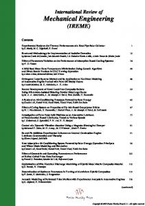
Example 3. Thermoelectric generator The thermal efficiency (h) = (electrical power out) / (thermal power in) of a thermoelectric power generation device (used in outer planetary spacecraft (Figure 2), powered by heat generated from radioisotope decay, typically plutonium-238) is given by

$ T ' 1+ ZTa −1 T + TH η = &1− L ) ; Ta ≡ L 2 % TH ( 1+ ZTa +T L /TH

(Equation 9)

where T is the temperature, the subscripts L, H and a refer to cold-side (low temperature), hot-side (high temperature) and average respectively, and Z is the “thermoelectric figure of merit”:

€

Z=

S2 ρk

(Equation 10)

where S is the Seebeck coefficient of material (units Volts/K, indicates how many volts are produced for each degree of temperature change across the material), r is the electrical resistivity (units ohm m) € (not to be confused with density!) and k is the material’s thermal conductivity (W/mK). (a) show that the units are valid (passes smoke test) Everything is obviously dimensionless except for ZTa, which must itself be dimensionless so that I can add it to 1. Note

15

# Volt &2 # J / coul &2 1 1 % ( % ( K 2 2 2 S J coul 1 K2 $ K ' $ K ' Z= Ta = K= K= 2 = 1 OK #W & # Js &# ( J / s) & 1 s(1/ s) 1 ρk J (ohm m)%$ mK (' %$ coul 2 m('%$ mK (' K coul 2

(b) €

show that the equation makes physical sense (passes function test) o If the material Z = 0, it produces no electrical power thus the efficiency should be zero. If Z = 0 then

$ T ' $ T ' $ T ' 1+ 0Ta −1 1 −1 0 η = &1− L ) = &1− L ) = &1− L ) =0 % TH ( 1+ 0Ta +T L /TH % TH ( 1 +T L /TH % TH ( 1+T L /TH

€

o If TL = TH, then there is no temperature difference across the thermoelectric material, and thus no power can be generated. In this case

η = (1−1)

€

OK

1+ ZTa −1 1+ ZTa + 1

= (0)

1+ ZTa −1 1+ ZTa + 1

=0

OK

o Even the best possible material (ZTa ® ∞) cannot produce an efficiency greater than the theoretically best possible efficiency (called the Carnot cycle efficiency, see page 86) = 1 – TL/TH, for the same temperature range. As ZTa ® ∞,

% T ( % T ( ZTa ZTa −1 T η ≈ '1− L * ≈ '1− L * = 1− L TH & TH ) ZTa +T L /TH & TH ) ZTa

OK

Side note #1: a good thermoelectric material such as Bi2Te3 has ZTa ≈ 1 and works up to about 200˚C before it starts to melt, thus

€ $ T ' $ T ' 1+ 1 −1 η = &1− L ) = 0.203&1− L ) = 0.203ηCarnot % TH ( 1+ 1 + (25 + 273) /(200 + 273) % TH ( $ 25 + 273 ' = 0.203&1− ) = 0.0750 = 7.50% % 200 + 273 ( By comparison, your car engine has an efficiency of about 25%. So practical thermoelectric materials are, in general, not very good sources of electrical power, but are extremely useful in some € niche applications, particularly when either (1) it is essential to have a device with no moving parts or (2) a “free” source of thermal energy at relatively low temperature is available, e.g. the exhaust of an internal combustion engine. Side note #2: a good thermoelectric material has a high S, so produces a large voltage for a small temperature change, a low r so that the resistance of the material to the flow of electric current is

16

low, and a low k so that the temperature across the material DT is high. The heat transfer rate (in Watts) q = kADT/Dx (see Chapter 7) where A is the cross-sectional area of the material and Dx is its thickness. So for a given DT, a smaller k means less q is transferred across the material. One might think that less q is worse, but no. Consider this: The electrical power = IV = (V/R)V = V2/R = (SDT) 2/(rDx/A) = S2DT2A/rDx. The thermal power = kADT/Dx The ratio of electrical to thermal power is [S2DT2A/rDx]/[kADT/Dx] = (S2/rk)DT = ZDT, which is why Z is the “figure of merit” for thermoelectric generators.)

Figure 2. Radioisotope thermoelectric generator used for deep space missions. Note that the plutonium-238 radioisotope is called simply, “General Purpose Heat Source.” Example 4. Density of matter Estimate the density of a neutron. Does the result make sense? The density of a white dwarf star is about 2 x 1012 kg/m3 – is this reasonable? The mass of a neutron is about one atomic mass unit (AMU), where a carbon-12 atom has a mass of 12 AMU and a mole of carbon-12 atoms has a mass of 12 grams. Thus one neutron has a mass of

"1 C -12 atom %" %" 12 g C -12 %" 1 kg % 1 mole C -12 -27 '$ '$ '$ ' = 1.66 ×10 kg 23 # 12 AMU &# 6.02 ×10 atoms C -12 &# mole C -12 Ϩ g &

(1 AMU)$

A neutron has a radius (r) of about 0.8 femtometer = 0.8 x 10-15 meter. Treating the neutron as a sphere, the volume is 4πr3/3, and the density (r) is the mass divided by the volume, thus

€

17

mass 1.66 ×10 -27 kg kg ρ= = = 7.75 ×1017 3 3 4 π volume m (0.8 ×10−15 m) 3 By comparison, water has a density of 103 kg/m3, so the density of a neutron is far higher (by a factor of 1014) than that of atoms including their electrons. This is expected since the nucleus of an € atom occupies only a small portion of the total space occupied by an atom – most of the atom is empty space where the electrons reside. Also, even the density of the white dwarf star is far less than the neutrons (by a factor of 105), which shows that the electron structure is squashed by the mass of the star, but not nearly down to the neutron scale (protons have a mass and size similar to neutrons, so the same point applies to protons too.)

18

Chapter 4. Forces in structures “The Force can have a strong influence on the weak-minded” - Ben Obi-wan Kenobi, explaining to Luke Skywalker how he made the famous “these aren’t the Droids you’re looking for” Jedi Mind Trick work. Main course in AME curriculum on this topic: AME 201 (Statics).

Forces Forces acting on objects are vectors that are characterized by not only a magnitude (e.g. Newtons or pounds force) but also a direction. A force vector F (vectors are usually noted by a boldface letter) can be broken down into its components in the x, y and z directions in whatever coordinate system you’ve drawn: F = Fxi + Fyj + Fzk

Equation 11

Where Fx, Fy and Fz are the magnitudes of the forces (units of force, e.g. Newtons or pounds force) in the x, y and z directions and i, j and k are the unit vectors in the x, y and z directions (i.e. vectors whose directions are aligned with the x, y and z coordinates and whose magnitudes are exactly 1 (no units)). Forces can also be expressed in terms of the magnitude = (Fx2 + Fy2 + Fz2)1/2 and direction relative to the positive x-axis (= tan-1(Fy/Fx) in a 2-dimensional system). Note that the tan-1(Fy/Fx) function gives you an angle between +90˚ and -90˚ whereas sometimes the resulting force is between +90˚ and +180˚ or between -90˚ and -180˚; in these cases you’ll have to examine the resulting force and add or subtract 180˚ from the force to get the right direction.

Degrees of freedom Imagine a one-dimensional (1D) world, i.e. where objects can move (translate) back and forth along a single line but in no other way. For this 1D world there is only one direction (call it the xdirection) that the object can move linearly and no way in which it can rotate, hence only one force balance equation is required. For the field of dynamics this equation would be Newton’s Second Law, namely that the sum of the forces Fx,1 + Fx,2 + Fx,3 + … + Fx,n = max where m is the mass of the object and ax is the acceleration of the object in the x direction, but this chapter focuses exclusively on statics, i.e. objects that are not accelerating, hence the force balance becomes simply n

∑F

x,i

=0

Equation 12.

i=1

19

So a 1D world is quite simple, but what about a 2D world? Do we just need a second force balance equation for translation in the y direction (that is, SFy = 0) and we’re done? Well, no. Let’s look at a counter-example (Figure 3). The set of forces on the object in the left panel satisfies the requirements SFx = 0 and SFy = 0 and would appear to be in static equilibrium. In the right panel, it is also true that SFx = 0 and SFy = 0, but clearly this object would not be stationary; instead it would be rotating clockwise. Why is this? In two dimensions, in addition to the translational degrees of freedom in the x and y directions, there is also one rotational degree of freedom, that is, the object can rotate about an axis perpendicular to the x-y plane, i.e., an axis in the z-direction. How do we ensure that the object is not rotating? We need to account for the moments of force (M) (discussed below in the next sub-section) in addition to the forces themselves, and just as the forces in the x and y directions must add up to zero, i.e. SFx = 0 and SFy = 0, we need to have the moments of force add up to zero, i.e. SM = 0. So to summarize, in order to have static equilibrium of an object, the sum of all the forces AND the moments of force must be zero. In other words, there are two ways that a 2-dimensional object can translate (in the x and y directions) and one way that in can rotate (with the axis of rotation perpendicular to the x-y plane.) So there are 3 equations that must be satisfied in order to have equilibrium, n

m

∑F

x,i

i=1

p

= 0;∑ Fy,i = 0; ∑ M i,A = 0 i=1

Equation 13

i=1

where the number of forces in the x direction is n, the number of forces in the y direction is m and p = n + m is the number of moments of force calculated with respect to some point A in the (x,y) plane. (The choice of location of point A is discussed below, but the bottom line is that any point yields the same result. 200 lbf

200 lbf

50 lbf

50 lbf

100 lbf

50 lbf

50 lbf

200 lbf

100 lbf

0 lbf

Figure 3. Two sets of forces on an object, both satisfying SFx = 0 and SFy = 0, but one (left) in static equilibrium, the other (right) not in static equilibrium. This is all fine and well for a 2D (planar) situation, what about 3D? For 3D, there are 3 directions an object can move linearly (translate) and 3 axes about which it can rotate, thus we need 3 force balance equations (in the x, y and z directions) and 3 moment of force balance equations (one each about the x, y and z axes.) Table 1 summarizes these situations.

20

# of spatial dimensions 1 2 3

Maximum # of force balances 1 2 3

Minimum # of moment of force balances 0 1 3

Total # of unknown forces & moments 1 3 6

Table 1. Number of force and moment of force balance equations required for static equilibrium as a function of the dimensionality of the system. (But note that, as just described, moment of force balance equations can be substituted for force balance equations.)

Moments of forces Some types of structures can only exert forces along the line connecting the two ends of the structure, but cannot exert any force perpendicular to that line. These types of structures include ropes, ends with pins, and bearings. Other structural elements can also exert a force perpendicular to the line (Figure 4). This is called the moment of force (often shortened to just “moment”, but to avoid confusion with “moment” meaning a short period of time, we will use the full term “moment of force”) which is the same thing as torque. Usually the term torque is reserved for the forces on rotating, not stationary, shafts, but there is no real difference between a moment of force and a torque. The distinguishing feature of the moment of force is that it depends not only on the vector force itself (Fi) but also the distance (di) from that line of force to a reference point A. (I like to call this distance the moment arm) from the anchor point at which it acts. If you want to loosen a stuck bolt, you want to apply whatever force your arm is capable of providing over the longest possible di. The line through the force Fi is called the line of action. The moment arm is the distance (di again) between the line of action and a line parallel to the line of action that passes through the anchor point. Then the moment of force (Mi) is defined as

A d

Line of action

Force Fi Figure 4. Force, line of action and moment of force (= Fd) about a point A. The example shown is a counterclockwise moment of force, i.e. force Fi is trying to rotate the line segment d counterclockwise about point A. 21

Mi = Fidi

Equation 14

where Fi is the magnitude of the vector F. Note that the units of Mo is force x length, e.g. ft lbf or N m. This is the same as the unit of energy, but the two have nothing in common – it’s just coincidence. So one could report a moment of force in units of Joules, but this is unacceptable practice – use N m, not J. Note that it is necessary to assign a sign to Mi depending on whether the moment of force is trying to rotate the free body clockwise or counter-clockwise. Typically we will define a clockwise moment of force as positive and counterclockwise as negative, but one is free to choose the opposite definition – as long as you’re consistent within an analysis. Note that the moment of forces must be zero regardless of the choice of the origin (i.e. not just at the center of mass). So one can take the origin to be wherever it is convenient (e.g. make the moment of one of the forces = 0.) Consider the very simple set of forces below: 200 lbf 0.707 ft

0.707 ft

A 45˚

0.5 ft 1 ft

B

0.5 ft

C 45˚

0.5 ft 0.707 ft

0.707 ft

141.4 lbf

141.4 lbf

D Figure 5. Force diagram showing different ways of computing moments of force Because of the symmetry, it is easy to see that this set of forces constitutes an equilibrium condition. When taking moments of force about point ‘B’ we have: SFx = +141.4 cos(45˚) lbf + 0 - 141.4 cos(45˚) lbf = 0 SFy = +141.4 sin(45˚) lbf - 200 lbf + 141.4 sin(45˚) = 0 SMB = -141.4 lbf * 0.707 ft - 200 lbf * 0 ft +141.4 lbf * 0.707 ft = 0. But how do we know to take the moments of force about point B? We don’t. But notice that if we take the moments of force about point ‘A’ then the force balances remain the same and SMA = -141.4 lbf * 0 ft - 200 lbf * 1 ft + 141.4 lbf * 1.414 ft = 0. The same applies if we take moments of force about point ‘C’, or a point along the line ABC, or even a point NOT along the line ABC. For example, taking moments of force about point ‘D’,

22

SMD = -141.4 lbf * (0.707 ft + 0.707 ft) + 200 lbf * 0.5 ft +141.4 lbf * 0.707 ft = 0 The location about which to take the moments of force can be chosen to make the problem as simple as possible, e.g. to make some of the moments of forces = 0. Example of “why didn’t the book just say that…?” The state of equilibrium merely requires that 3 constraint equations are required. There is nothing in particular that requires there be 2 force and 1 moment of force constraint equations. So one could have 1 force and 2 moment of force constraint equations: n

n

∑F i=1

n

x, i = 0;∑ M i, A = 0; ∑ M j, B = 0 i=1

Equation 15

j=1

where the coordinate direction x can be chosen to be in any direction, and moments of force are taken about 2 separate points A and B. Or one could even have 3 moment of force equations: €

n

∑M i=1

n i, A

n

= 0; ∑ M j, B = 0; ∑ M j,C = 0 j=1

Equation 16

j=1

Also, there is no reason to restrict the x and y coordinates to the horizontal and vertical directions. They can be (for example) parallel and perpendicular to an inclined surface if that appears in the € problem. In fact, the x and y axes don’t even have to be perpendicular to each other, as long as they are not parallel to each other, in which case SFx = 0 and SFy = 0 would not be independent equations.

Types of forces and moments of force A free body diagram is a diagram showing all the forces and moments of forces acting on an object. We distinguish between two types of objects: 1. Particles that have no spatial extent and thus have no moment arm (d). An example of this would be a satellite orbiting the earth because the spatial extent of the satellite is very small compared to the distance from the earth to the satellite or the radius of the earth. Particles do not have moments of forces and thus do not rotate in response to a force. 2. Rigid bodies that have a finite dimension and thus has a moment arm (d) associated with each applied force. Rigid bodies have moments of forces and thus can rotate in response to a force. There are several types of forces that act on particles or rigid bodies: 1. Rope, cable, etc. – Force (tension) must be along line of action; no moment of force (1 unknown force)

T

23

2. Rollers, frictionless surface – Force must be perpendicular to the surface; no moment of force (1 unknown force). There cannot be a force parallel to the surface because the roller would start rolling! Also the force must be away from the surface towards the roller (in other words the roller must exert a force on the surface), otherwise the roller would lift off of the surface.

F

3. Frictionless pin or hinge – Force has components both parallel and perpendicular to the line of action; no moment of force (2 unknown forces) (note that the coordinate system does not need to be parallel and perpendicular to either the gravity vector or the bar) Fy

Fx

4. Fixed support – Force has components both parallel and perpendicular to line of action plus a moment of force (2 unknown forces, 1 unknown moment force). Note that for our simple statics problems with 3 degrees of freedom, if there is one fixed support then we already have 3 unknown quantities and the rest of our free body cannot have any unknown forces if we are to employ statics alone to determine the forces. In other words, if the free body has any additional unknown forces the system is statically indeterminate as will be discussed shortly. Fy

M

Fx

5. Contact friction – Force has components both parallel (F) and perpendicular (N) to surface, which are related by F = µN, where µ is the coefficient of friction, which is usually 24

assigned separate values for static (no sliding) (µs) and dynamic (sliding) (µd) friction, with the latter being lower. (2 unknown forces coupled by the relation F = µN). µ depends on both of the surfaces in contact. Most dry materials have friction coefficients between 0.3 and 0.6 but Teflon in contact with Teflon, for example, can have a coefficient as low as 0.04. Rubber (e.g. tires) in contact with other surfaces (e.g. asphalt) can yield friction coefficients of almost 2.

N

N

F = µN

F = µN

Actually the statement F = µsN for static friction is not correct at all, although that’s how it’s almost always written. Consider the figure on the right, above. If there is no applied force in the horizontal direction, there is no need for friction to counter that force and keep the block from sliding, so F = 0. (If F ≠ 0, then the object would start moving even though there is no applied force!) Of course, if a force were applied (e.g. from right to left, in the –x direction) then the friction force at the interface between the block and the surface would counter the applied force with a force in the +x direction so that SFx = 0. On the other hand, if a force were applied from left to right, in the +x direction) then the friction force at the interface between the block and the surface would counter the applied force with a force in the -x direction so that SFx = 0. The expression F = µsN only applies to the maximum magnitude of the static friction force. In other words, a proper statement quantifying the friction force would be |F| ≤ µsN, not F = µsN. If any larger force is applied then the block would start moving and then the dynamic friction force F = µdN is the applicable one – but even then this force must always be in the direction opposite the motion – so |F| = µdN is an appropriate statement. Another, more precise way of writing this would be     v v F = µ d N , where v is the velocity of the block and v is the magnitude of this velocity, thus is a v v unit vector in the direction of motion. Special note: while ropes, rollers and pins do not exert a moment of force at the point of contact, you can still sum up the moments of force acting on the free body at that point of contact. In other words, SMA = 0 can be used even if point A is a contact point with a rope, roller or pin joint, and all of the other moments of force about point A (magnitude of force x distance from A to the line of action of that force) are still non-zero. Keep in mind that A can be any point, within or outside of the free body. It does not need to be a point where a force is applied, although it is often convenient to use one of those points as shown in the examples below. Statically indeterminate system Of course, there is no guarantee that the number of force and moment of force balance equations will be equal to the number of unknowns. For example, in a 2D problem, a beam supported by one pinned end and one roller end has 3 unknown forces and 3 equations of static equilibrium. However, if both ends are pinned, there are 4 unknown forces but still only 3 equations of static 25

equilibrium. Such a system is called statically indeterminate and requires additional information beyond the equations of statics (e.g. material stresses and strains, discussed in the next chapter) to determine the forces.

Analysis of statics problems A useful methodology for analyzing statics problems is as follows: 1. Draw a free body diagram – a free body must be a rigid object, i.e. one that cannot bend in response to applied forces 2. Draw all of the forces acting on the free body. Is the number of unknown forces equal to the total number of independent constraint equations shown in Table 1 (far right column)? If not, statics can’t help you. 3. Decide on a coordinate system. If the primary direction of forces is parallel and perpendicular to an inclined plane, usually it’s most convenient to have the x and y coordinates parallel and perpendicular to the plane, as in the cart and sliding block examples below. 4. Decide on a set of constraint equations. As mentioned above, this can be any combination of force and moment of force balances that add up to the number of degrees of freedom of the system (Table 1). 5. Decide on the locations about which to perform moment of force constraint equations. Generally you should make this where the lines of action of two or more forces intersect because this will minimize the number of unknowns in your resulting equation. 6. Write down the force and moment of force constraint equations. If you’ve made good choices in steps 2 – 5, the resulting equations will be “easy” to solve. 7. Solve these “easy” equations. Example 1. Ropes Two tugboats, the Monitor and the Merrimac, are pulling a Peace Barge due west up Chesapeake Bay toward Washington DC. The Monitor’s tow rope is at an angle of 53 degrees north of due west with a tension of 4000 lbf. The Merrimac’s tow rope is at an angle of 34 degrees south of due west but their scale attached to the rope is broken so the tension is unknown to the crew.

26

y

Monitor 4000 lbf

53˚ x 34˚ Merrimac

Barge

??? lbf

Figure 6. Free body diagram of Monitor-Merrimac system a) What is the tension in the Merrimac’s tow rope? Define x as positive in the easterly direction, y as positive in the northerly direction. In order for the Barge to travel due west, the northerly pull by the Monitor and the Southerly pull by the Merrimac have to be equal, or in other words the resultant force in the y direction, Ry, must be zero. The northerly pull by the Monitor is 4000 sin(53˚) = 3195 lbf. In order for this to equal the southerly pull of the Merrimac, we require FMerrimacsin(34˚) = 3195 lbf, thus FMerrimac = 5713 lbf. b) What is the tension trying to break the Peace Barge (i.e. in the north-south direction)? This is just the north/south force just computed, 3195 lbf c) What is the force pulling the Peace Barge up Chesapeake Bay? The force exerted by the Monitor is 4000 cos(53˚) = 2407 lbf. The force exerted by the Merrimac is 5713 cos(34˚) = 4736 lbf. The resultant is Rx = 7143 lbf. d) Express the force on the Merrimac in polar coordinates (resultant force and direction, with 0˚ being due east, as is customary) The magnitude of the force is 5713 lbf as just computed. The angle is -180˚ - 34˚ = -146˚. Example 2. Rollers A car of weight W is being held by a cable with tension T on a ramp of angle q with respect to horizontal. The wheels are free to rotate, so there is no force exerted by the wheels in the direction parallel to the ramp surface. The center of gravity of the vehicle is a distance “c” above the ramp, a distance “a” behind the front wheels, and a distance “b” in front of the rear wheels. The cable is attached to the car a distance “d” above the ramp surface and is parallel to the ramp.

27

T d

c

A a Fy,A

W y b B x Fy,B

θ

Figure 7. Free body diagram for car-on-ramp with cable example (a) What is the tension in the cable in terms of known quantities, i.e. the weight W, dimensions a, b, c, and d, and ramp angle q? Define x as the direction parallel to the ramp surface and y perpendicular to the surface as shown. The forces in the x direction acting on the car are the cable tension T and component of the vehicle weight in the x direction = Wsinq, thus SFx = 0 yields Wsinq - T = 0 Þ T = Wsinq (b) What are the forces where the wheels contact the ramp (Fy,A and Fy,B)? The forces in the y direction acting on the car are Fy,A, Fy,B and component of the vehicle weight in the y direction = Wcosq. Taking moments of force about point A, that is SMA = 0 (so that the moment of force equation does not contain Fy,A which makes the algebra simpler), and defining moments of force as positive clockwise yields (Wsinq)(c) + (Wcosq)(a) – Fy,B(a+b) – T(d) = 0 Since we already know from part (a) that T = Wsinq, substitution yields (Wsinq)(c) + (Wcosq)(a) – Fy,B(a+b) – (Wsinq)(d) = 0 Since this equation contains only one unknown force, namely Fy,B, it can be solved directly to obtain Fy,B = W

a cos(θ ) + (c − d)sin(θ ) a+b

28

Finally taking SFy = 0 yields Fy,A + Fy,B - Wcosq = 0 Which we can substitute into the previous equation to find Fy,A: Fy,A = W

b cos(θ ) − (c − d)sin(θ ) a+b

Note the function tests: 1) For q = 0, T = 0 (no tension required to keep the car from rolling on a level road) 2) As q increases, the tension T required to keep the car from rolling increases 3) For q = 90˚, T = W (all of the vehicle weight is on the cable) but note that Fy,A and Fy,B are non-zero (equal magnitudes, opposite signs) unless c = d, that is, the line of action of the cable tension goes through the car’s center of gravity. 4) For q = 0, Fy,A = (b/(a+b)) and Fy,B = (a/(a+b)) (more weight on the wheels closer to the center of gravity.) 5) Because of the – sign on the 2nd term in the numerator of Fy,A (-(c-d)sin(q)) and the + sign in the 2nd term in the numerator of Fy,B (+(c-d)sin(q)), as q increases, there is a transfer of weight from the front wheels to the rear wheels. Note also that Fy,A < 0 for b/(c-d) < tan(q), at which point the front (upper) wheels lift off the ground, and that Fy,A < 0 for a/(d-c) > tan(q), at which point the back (lower) wheels lift off the ground. In either case, the analysis is invalid. (Be aware that c could be larger or smaller than d, so c-d could be a positive or negative quantity.) Example 3. Friction A 100 lbf acts on a 300 lbf block placed on an inclined plane with a 3:4 slope. The coefficients of friction between the block and the plane are µs = 0.25 and µd = 0.20. a) Determine whether the block is in equilibrium b) If the block is not in equilibrium (i.e. it’s sliding), find the net force on the block c) If the block is not in equilibrium, find the acceleration of the block

29

y

300 lbf N

x F = µN

100 lbf 5

3

4

Figure 8. Free body diagram for sliding-block example (a) To maintain equilibrium, we require that SFx = 0 and SFy = 0. Choosing the x direction parallel to the surface and y perpendicular to it, SFy = N – (4/5)(300 lbf) = 0 Þ N = 240 lbf so the maximum possible friction force is Ffriction, max = µsN = 0.25 * 240 lbf = 60 lbf. The force needed to prevent the block from sliding is SFx = 100 lbf – (3/5)(300 lbf) + Fneeded = 0 Fneeded = -100 lbf + (3/5)(300 lbf) = 80 lbf Which is more than the maximum available friction force, so the block will slide down the plane. (b) The sliding friction is given by Ffriction, max = µdN = 0.20 * 240 lbf = 48 lbf so the net force acting on the block in the x direction (not zero since the block is not at equilibrium) is SFx = 100 lbf – (3/5)(300 lbf) + 48 lbf = -32 lbf (c) F = ma Þ -32 lbf = 300 lbm * acceleration acceleration = (-32 lbf/300 lbm) ??? what does this mean? lbf/lbm has units of force/mass, so it is an acceleration. But how to convert to something useful like ft/s2? Multiply by 1 in the funny form of gc = 1 = 32.174 lbm ft / lbf s2, of course!

30

acceleration = (-32 lbf/300 lbm) (32.174 lbm ft / lbf s2) = -3.43 ft/s2 or, since gearth = 32.174 ft/s2, acceleration = (-3.43 ft/s2)/(32.174 ft/s2gearth) = -0.107 gearth. The negative sign indicates the acceleration is in the –x direction, i.e. down the slope of course. A good function test is that the acceleration has to be less than 1 gearth, which is what you would get if you dropped the block vertically in a frictionless environment. Obviously a block sliding down a slope (not vertical) with friction and with an external force acting up the slope must have a smaller acceleration. Example 4. Rollers and friction A car of weight W is equipped with rubber tires with coefficient of static friction µs. Unlike the earlier example, there is no cable but the wheels are locked and thus the tires exert a friction force parallel to and in the plane of the ramp surface. As with the previous example, the car is on a ramp of angle q with respect to horizontal. The center of gravity of the vehicle is a distance “c” above the ramp, a distance “a” behind the front wheels, and a distance “b” in front of the rear wheels.

µFy,A

c

A a Fy,A

W µFy.B b B Fy,B

θ

Figure 9. Free body diagram for car-on-ramp with friction example (a) What is the minimum µs required to keep the car from sliding down the ramp? The unknowns are the resulting forces at the wheels (Fy,A and Fy,B) and the coefficient of friction µs. Taking SFx = 0, SFy = 0 and SMA = 0 yields, respectively,

31

-µsFy,A - µsFy,B + Wsinq = 0 Fy,A + Fy,B - Wcosq = 0 (Wsinq)(c) + (Wcosq)(a) – Fy,B(a+b) = 0 Which may be solved to obtain Fy,A = W

bcos(θ ) − c sin(θ ) acos(θ ) + c sin(θ ) sin(θ ) ;Fy,B = W ; µs = = tan(θ ) a+b a+b cos(θ )

Note the function tests €

1) For q = 0, µs = tan(q) = 0 (no friction required to keep the car from sliding on a level road) 2) As q increases, the friction coefficient µs required to keep the car from sliding increases 3) For q = 0, Fy,A = (b/(a+b)) and Fy,B = (a/(a+b)) (more weight on the wheels closer to the center of gravity 4) Because of the – sign on the 2nd term in the numerator of Fy,A (-c sin(q)) and the + sign in the 2nd term in the numerator of Fy,B (+c sin(q)), as q increases, there is a transfer of weight from the front wheels to the rear wheels. Note also that we could have also tried SFy = 0, SMA and SMB = 0: Fy,A + Fy,B - Wcosq = 0 (Wsinq)(c) + (Wcosq)(a) – Fy,B(a+b) = 0 (Wsinq)(c) - (Wcosq)(b) + Fy,A(a+b) = 0 In which case, the second equation could have been subtracted from the third to obtain: Fy,A + Fy,B - Wcosq = 0 which is the same as the first equation. So the three equations are not independent of each other, and we can’t solve the system. What’s wrong? The coefficient of friction µs doesn’t appear in the set of equations SFx = 0, SMA and SMB = 0. We need to have each of the three unknowns Fy,A, Fy,B and µs in at least one of the three equations. The set SFx = 0, SMA and SMB = 0 doesn’t satisfy that criterion. (b) At what angle will the car tip over backwards, assuming that it doesn’t start sliding down the ramp at a smaller angle due to low µs? This will occur when Fy,A = 0, i.e. when sin(q)/cos(q) = tan(q) = b/c. This is reasonable because the tip-over angle should increase when c is made larger (center of gravity closer to the ground) or b made smaller (center of gravity shifted forward). Notice also that it doesn’t

32

depend on µs, that is, as long as it doesn’t slide due to low µs, the tip-over angle only depends on the force balance. For what it’s worth, also note that the tip-over angle equals the sliding angle when tan(q) = µs = b/c. Since generally µs < 1, except for a very top-heavy (large c) or rear-weight-shifted (small b) vehicles, the vehicle will slide down the ramp before it flips over backwards. Example 5. Pinned joint

B

12 in

4 in

6 in

C 30˚

A

4 cos(30)

8 cos(30)

100 lbf

Figure 10. Free body diagram for pinned joint example A straight bar of negligible mass 12 inches long is pinned at its lower end (call it point A) and has a roller attached to its upper end (call it point B) as shown in the figure. The bar is at a 30˚ angle from horizontal. A weight of 100 lbf is hung 4 inches from the lower end (call it point C). a) What are the forces in the x and y directions on the pinned end? What is the force in the x direction on the roller end? The pinned end can sustain forces in both the x and y directions, but no moment of force. The roller end can sustain a force only in the x direction, and again no moment of force. Summing the forces in the y direction Fy,A + Fy,B + Fy,C = 0 Þ Fy,A + 0 - 100 lbf = 0 Þ Fy,A = +100 lbf. In other words, in the y direction the vertical force at point A must be +100 lbf since that is the only force available to counteract the 100 lbf weight. Next, taking moments of force about point A (since the lines of action of two of the unknown forces intersect at point A), SMA = 0 Þ +(4 in)(cos(30˚))(100 lbf) + (6 in)Fx,B = 0 Þ Fx,B = -57.7 lbf. Finally, for force balance in the x direction, Fx,A + Fx,B + Fx,C = 0 Þ Fx,A = -Fx,B - Fx,C = -(-57.7 lbf) – 0 = +57.7 lbf 33

b) Would the forces change if the roller and pinned ends were reversed? In this case summing the forces in the x direction: Fx,A + Fx,B + Fx,C = 0 Þ 0 + Fx,B + 0 = 0 Þ Fx,B = 0. For force balance in the y direction, Fy,A + Fy,B + Fy,C = 0 Þ Fy,A + Fy,B = 100 lbf Taking moments of force about point C just for variety (not the easiest way, since neither Fy,A nor Fy,B are known, we just know that Fy,A + Fy,B = 100 lbf), SMC = 0 Þ (4 in)(cos(30˚))Fy,A - (8 in)(cos(30˚))Fy,B + (8 in)(sin(30˚))Fx,B = 0 Þ (4 in)(cos(30˚))(100 lbf – Fy,B) - (8 in)(cos(30˚))Fy,B + 0 = 0 Þ Fy,B = +33.3 lbf Þ Fy,A = +66.7 lbf which is quite different from case (a). c) What would happen if the lower end were fixed rather than pinned (upper end having the roller again)? In this case there are 4 unknown quantities (Fx,A, Fy,A, MA and Fx,B) but only 3 equations (SFx = 0, SFy = 0, SM = 0) so the system is statically indeterminate. If one takes away the roller end entirely, then obviously Fy,A = 100 lbf, Fx,A = 0 and MA = +(100 lbf)(4 in)(cos(30˚)) = 346.4 in lbf.

34

Chapter 5. Stresses, strains and material properties “It is not stress that kills us, it is our reaction to it” - Hans Selye, endocrinologist. Main course in AME curriculum on this topic: AME 204 (Strength of Materials).

Stresses and strains As a follow-on to the discussion of statics we need to consider whether a material subject to a given set of forces will break and if not, how much will it bend? While we will write down many formulas in this chapter without deriving them, essentially what we will do is apply the laws of statics you just learned to an infinitesimal cube of material, and sum up the effects of these tiny cubes to determine the forces acting on a material of a particular size and shape being poked and prodded by some forces. The first step is to compute the stress in the material. There are two flavors of stress, the normal stress which is the stress in the direction perpendicular to an imaginary plane in the material, and the shear stress which is the stress in the direction parallel to that same imaginary plane. Of course, this imaginary plane could be in any direction, so the magnitude of the normal and shear stresses depends strongly on the choice of said imaginary plane. How should one choose said plane and what is the relationship between normal and shear stresses? We’ll discuss that shortly, but first we’ll individually define normal then shear stress. The normal stress (s) in a material is defined as s º F/A

Equation 17

where F is the force (either tension or compression) acting perpendicular to an imaginary plane surface passing through a piece of material and A is the cross section area. It is called “normal” not in the sense of being “typical” or “standard” but in the sense of being perpendicular or orthogonal to the cross-section of the material. Stress is defined as positive if the material is in tension (i.e. the material is being pulled apart) and negative if the material is in compression (i.e. being squeezed together). From the definition it is clear that stress has units of force/area, i.e. the same as pressure. The units are typically N/m2 or lbf/in2. Sometimes the unit of “kips” (kilopounds per square inch = 1000 lbf/in2) is used to report stress. In order to characterize the deformation of a material in response to stress we define another property called strain (e) which is the fractional amount of elongation (increase in length) or contraction (decrease in length) in a material caused by a stress. For example, if under a given amount of tensile stress, a steel bar stretches from a length (L) of 1.00 inch to 1.01 inch (a change in length, DL, of 0.01 inch) the strain = (1.01 – 1.00)/1.00 = 0.01. In other words, e º DL/L

Equation 18

35

For most materials (other than gooey ones, i.e. Silly Putty™, Play-Doh™, …) the amount of strain before failure is relatively small (i.e. less that 0.1, meaning that the material deforms less than 10% before failing.) An elastic material has a linear relationship between stress and strain, i.e. s = eE

Equation 19

where E is called the elastic modulus, i.e. the slope of the plot of s vs. e in the elastic region shown in Figure 11. Note that since e is dimensionless, E also has units of force per unit area. The strength of a material is generally reported in terms of the maximum stress it can withstand. For a sufficiently small stress, materials return to their original length or shape after the stress is removed. The smallest stress for which the material does not return to its original length or shape after the stress is removed is called the yield stress (syield). Beyond this stress, generally the slope of the s vs. e plot generally (but not always) becomes smaller. There is often an increase in slope as e is increased still further, up to a maximum s called the “ultimate stress”, beyond which s actually decreases as e increases, leading finally to fracture (breakage) of the material at which point it can no longer hold any stress. A material’s yield stress may be (and usually is) different in tension, compression and shear. Note that we can write the above equation s = eE in the form F/A = (DL/L)E or F = (EA/L)(DL), which looks just like the force on a linear spring, F = kx, with k = EA/L. (One might wonder what happened to the – sign, that is, isn’t F = -kx? Stress is usually defined as positive in tension where as for the spring F is defined as positive in compression.) So E and the material dimensions A and L determine its “spring constant.” Figure 11 shows examples of stress vs. strain (s vs. e) relationships for different materials. A ductile material such as steel will yield significantly before fracture whereas a brittle material such as a ceramic or concrete will fail without significant yielding, that is, the s vs. e curve is nearly linear up to the failure point. This doesn’t mean that ceramics are necessary weak, in

Slope = E

Figure 11. Typical stress-strain relationships: left: ductile material; right: comparison of various types of materials. Sources: http://dolbow.cee.duke.edu/TENSILE/tutorial/node4.html, http://www.cyberphysics.co.uk/topics/forces/young_modulus.htm

36

fact they may have higher E than ductile materials, but they are unforgiving to over-stressing (really, over-straining.) E and yield or ultimate stress have the same units (Pa or lbf/in2) but there is no particular relationship between E and yield or ultimate stress. Materials can be hard (high E) but break easily (low yield or ultimate stress) or vice versa. Some examples of material properties are shown in Table 2. This table shows materials that are isotropic, i.e. their properties are similar no matter what direction stress is applied relative to the material. Many engineering materials are anisotropic, i.e. they are not isotropic. A typical example of such materials is graphite-epoxy composites composed of fibers of graphitic carbon (which have very high yield stress in the plane of the graphite sheets, and low yield stress in the direction perpendicular to this plane) that are bonded to an epoxy polymer, which has relatively low yield stress in tension but high yield stress in compression and shear. The result is a material that has very high stress for its weight. The Boeing 787 uses composites for most of the structure; this has the advantage of high ratio of yield stress to weight, no possibility of corrosion, and relative ease of forming into any desired shape. (One could also say that a much older material, namely wood, is also an anisotropic composite material.) Of course, in any design one must employ a material with a yield stress greater than the actual stress in the material; the ratio of the yield stress of the material to the actual predicted stress in the material is call the factor of safety. For example, if a material has a yield stress in tension of 10,000 lbf/in2 and the system is designed such that the maximum tension is 2,500 lbf/in2, the factor of safety for this particular design is (10,000 lbf/in2/2,500 lbf/in2) = 4, at least in tension. Some factoids about materials How strong are these materials? How does this compare with the strength of the attractive forces between the atoms (Fatoms)? That is, can we estimate the yield stress of the material s ≈ Fatoms/Aatoms, where Aatoms is the cross-section area of the atoms? How could we estimate Fatoms and Aatoms based on macroscopically measurable properties? Let’s start with the size of one atom. Let’s consider a typical material like aluminum. Its molecular weight is 27 g/mole, and its density is (by coincidence) 2.7 g/cm3, and 1 mole = 6.02 x 1023 atoms. So the volume occupied by each atom is Material Aluminum, 6061-T6 Steel, 4340-HR Iron, pure Diamond High-density polyethylene Alumina, Al2O3 Solder (60% tin, 40% lead) Silica aerogel

E (109 Pa)

n

68.9 200 200 700 – 1200 0.18 – 1.6

0.32 0.30 0.29 0.10 – 0.29

370 30

0.22 0.4

0.001 – 0.01

0.2

Yield stress (in tension unless otherwise noted) (106 Pa) 276 910 30 8680 – 16530 (compressive) 2.4 – 31.7

Ultimate stress (106 Pa) 310 1041 540

3000 (compressive)

300 53

10 – 50

Table 2. Properties of some common materials (from http://www.matweb.com) 37

0.016

3 cm 3 27g mole −23 cm = 1.66 ×10 2.7g mole 6.02 ×1023 atom atom

Thus each atom occupies a roughly cubic space of (1.66 x 10-23)1/3 = 2.55 x 10-8 cm = 2.55 x 10-10 m, or a cross-section area of (2.55 x 10-10 m)2 = 6.51 x 10-20 m2. What is the attractive force between the € atoms? The heat of formation of Al(gas) from Al(s) is 330 kJ/mole (see http://webbook.nist.gov). This is the energy needed to separate Al atoms in the solid phase from each other to make a gas. On a per-atom basis this is (330,000 J/mole)(mole/6.02 x 1023 atoms) = 5.48 x 10-19 J. Then, since Energy = force x distance, we can roughly estimate the attractive force as energy/distance or Fatoms = (5.48 x 10-19 J)/(2.55 x 10-10 m) = 2.15 x 10-9 N. Then finally, the force per unit area is Fatoms = (2.15 x 10-9 N)/(6.51 x 10-20 m2) = 3.30 x 1010 Pa = 33 GPa Note that this is comparable to the elastic modulus (E), not the yield stress in tension or shear, which is about 1000 times smaller. Why is the yield stress so much smaller than the elastic modulus? For a perfect crystal with no defects, the above estimate would be appropriate. But real materials have defects in their crystalline structure. The yield stress of materials is determined mostly by the microstructural properties like the number of defects, the size of the “grains” (individual crystals), and the response of the defects to strain. This is why small amounts of additives (like adding carbon to iron to make steel) to a material and the details of how the material is processed (e.g. heat treating, rolling, etc.) affect its yield stress so much, but do not significantly affect other properties such as E, n (see below), density, etc. You’ll learn much more about this in MASC 310. As materials deform under tension, they become longer of course, but they also become narrower. The ratio between the change in diameter (d) of a cylindrical sample and change in length (L) is called Poisson’s ratio (n), i.e.

ν ≡−

Δd d

ΔL L

Equation 20

The minus sign is there because under tension DL > 0 (sample lengthening) but Dd < 0 (sample is narrowing). Note that the volume (V) of the cylindrical sample is Lπd2/4 before applying the stress, and (L+DL)π(d+Dd)2/4 after applying the stress. So

(

)( (

)(

π / 4 L + ΔL d + Δd V + ΔV = V π / 4 Ld 2

)

2

)

or, keeping only terms with one Dd or DL (not (Dd)2, (Dd)(DL), (DL)2 etc.) ΔV Δd ΔL ΔL ⎛ Δd =2 + =2 ⎜ V d L L ⎝ d

ΔL ⎞ ΔL ΔL = 1− 2ν ⎟+ L⎠ L L

(

38

)

Equation 21

Function test. From the above equation, it is apparent that for a material to have no change in volume under stress, one would need 1 - 2n = 0 or n = 0.5. In reality most materials have n ≈ 0.3, which means that their volume increases under tensile load (DL/L > 0). Certainly one would not expect n > 0.5, for this would imply the volume decreases under tensile load, and increases under compressive load (DL/L < 0) – not very likely! Example A ½ inch diameter steel bar increases in length from 10 cm to 10.4 cm under an applied force of 10,000 lbf. (a) What is the stress in the bar? Stress = force/area = 10,000 lbf / (π(0.5 in)2/4) = 50920 lbf/in2. (b) What is the strain in the bar? Strain = DL/L = (10.4 cm – 10 cm)/(10 cm) = 0.04 (c) What is the change in diameter of the bar? Note that the volume of the bar isn’t constant; to answer this question you’ll have to use the expression for Poisson’s ratio given above. n º -(Dd/d)/(DL/L); if n ≈ 0.3 for steel as in Table 2, then Dd = -nd(DL/L) = -(0.3)(0.5 inch)((0.4 cm)/(10 cm)) = -0.006 inch Shear forces Tension and compression are forces that act in the direction perpendicular to a particular imaginary plane cut through a piece of material. The force that acts parallel to a particular imaginary plane cut through the material is called the shear force (V) (why V? I dunno…). The shear stress (t) is the shear force per unit area, i.e. t = V/A.

Equation 22

To describe all of the stresses (normal and shear) in a material, we need something more than just a vector (which sufficed to describe forces.) For example, a two-dimensional object in the x-y plane has two components of tension or compression (call them sx and sy) and two shear stresses (one each in the x and y directions; call them txy-x and txy-y; usually these are just called tyx and txy). These are 4 entities acting in the x-y plane; the composite effect of these 4 stresses cannot be represented in terms of a single scalar or vector. In three dimensions, the situation is even more problematic. As shown in Figure 12, a three-dimensional object will have three components of tension or compression (one each in the x, y and z directions) and six components of shear (in the x-y plane, in the x and y directions; in the y-z plane, in the y and z directions; and in the x-z plane, in the x and z

39

directions). So stress is actually not a single scalar value or even a single vector but a 3 x 3 matrix called the Cauchy stress tensor: $σ x & σ = &τ yx &%τ zx

τ xy τ xz ' ) σ y τ yz ) τ zy σ z )(

Equation 23

Keep in mind that for each force shown in Figure 12, there is an equal and oppositely-directed force on the opposing side of the imaginary cube. This looks fairly complicated, and perhaps it is, but one € saving grace is that, in order for the moments of force about a very small cube of material to sum to zero, one must have txy-x = tyx-y, tzx-z = txz-x and tzy-z = tyz-y, in other word the matrix is symmetric. So there are only 6, not 9, independent stresses, or in two dimensions there are only 3 independent stresses, namely sx, sy and txy = tyx. Note the analogy between the number of independent stresses (3 in two dimensions, 6 in three dimensions) and the number of degrees of freedom of a free body (see Table 1) which determines the number of constraint equations needed to enforce static equilibrium; this is not a coincidence at all but a necessary outcome of the number of degrees of freedom of an object as discussed in the previous chapter on Statics. Note that normal stress is defined as the stress in the direction perpendicular to an imaginary plane and shear stress is defined as the stress in the direction parallel to that same imaginary plane – but how should that plane be chosen? For a simple shape like a cylinder it seems natural to define a plane parallel to the ends of the cylinder, but what about oddly shaped objects? Will the stresses be different depending on how one chooses the coordinate system? Will an object fail or not fail under stress depending on how one chooses the coordinate system? What is important to learn from this sub-section is that the magnitudes of both normal stress and shear stress are entirely dependent on the choice of coordinate system. This is no different than simple forces; how much force is in the x-direction and how much is in the y-direction is entirely dependent on the choice of coordinate system.

y σy τyx τyz

τxy

τzy

σx τzx

τxz

x

σz z

Figure 12. Diagram of normal (s) and shear (t) stresses in an imaginary, infinitesimally small cube of material 40

Figure 13. Diagram of normal (s) and shear (t) stresses in a 2-dimensional system and transformation to the principal stresses. From http://www.efunda.com Principal Stresses It can be shown that the coordinate system (x, y, z) of Figure 12 can be rotated such that all of the off-diagonal terms (i.e. all the shear stresses t) are zero; these coordinates are called the principal directions and the corresponding stresses the principal stresses. Now we’re down to 3 independent stresses in this coordinate system. Furthermore, in the principal directions two of the three coordinates yield the maximum and minimum stress attainable from any rotation of the coordinates. Proving this or using these results is beyond the scope of this course; wait for AME 204. In this course we will consider only the simpler two-dimensional case (Figure 13). If the normal stresses sx and sy and the shear stress txy are known in some coordinate system (x, y) then by rotating the coordinate system by an angle qP, the principal stresses (called s1 and s2) are obtained; their values are given by σ1 =

2 2 "σ −σ y % "σ x −σ y % σ x +σ y σ x +σ y 1 −1 " 2τ xy % 2 2 '' + $ x + τ ; σ = − ' $ ' + τ xy ; θ P = tan $$ xy 2 2 2 2 # 2 & # 2 & #σ x −σ y &

Equation 24

Note that s1 and s2 could be both positive, both negative, or one of each depending on the values of sx,, sy and txy. If both are positive then the larger one is the only one you need to worry about in terms of material failure, and failure could occur in tension only. If both s1 and s2 are negative, then the more negative one is the only one you need to worry about in terms of material failure, and failure could occur in compression only. If s1 is positive and s2 is negative, then you need to worry about both in terms of material failure, the positive one in tension and the negative one in compression.

41

Also note that there are some good function tests you can perform on the formula for principal stresses: • • •

If txy =0, then s1 = sx and s2 = sy, that is, the normal stresses are the principal stresses since there is no shear in this coordinate systems. If sy and txy are both zero, that is, if there is only one normal stress and no shear stress, then s1 = sx and s2 =0. If sy = 0 but txy ≠ 0, then the principal stresses are

σ1 =

2 2 !σ $ !σ $ σx σ + # x & + τ xy2 > σ x , σ 2 = x − # x & + τ xy2 < 0 " 2 % " 2 % 2 2

which makes sense because adding the shear increases s1 to a value larger than its value if there were no shear (sx), and decreases s2 to a value smaller than its value if there were no shear (0). In other words, the addition of shear increases both the minimum and maximum normal stresses. Also, by rotating the coordinate system by a different angle qS, the maximum shear stress (tmax) is obtained; its value is given by

τ max

€

% σ x − σ y (2 2 σ1 − σ 2 1 −1% σ x − σ y ( ** = θ P ± 45˚ =± ' + τ = ± ; θ = tan '' * xy S 2 2 & 2 ) & 2τ xy )

Equation 25

In this coordinate system where we find the maximum shear stress, the normal stresses are the same and equal to (sx + sy)/2, i.e., the average of sx and sy in the original coordinate system. It is worth noting that for shear stresses txy we do not need to distinguish between positive and negative values since txy always appears in the equations in the form txy2 and tmax always has a ± sign in front of it. This is because (as Figure 12 indicates) only 1 type of shear stress txy = tyx is allowed; txy ≠ tyx would violate static equilibrium because the sum of moments of force would not be zero. In contrast, two independent normal stresses sx and sy are allowed and there is no restriction on their relative magnitudes or signs. Note also that if in the above equations the stress in the x direction is non-zero (sx ≠ 0) but the stress in the y direction is zero (sy = 0) and the shear in the x-y plane is zero (txy = 0), then the principal stresses are s1 = sx, s2 = 0 and tmax = sx/2. Note also that just because I’m only pulling on the material in one direction (say, in tension) that doesn’t mean that there is no shear stress in the material; it’s all a matter of my choice of coordinates. The important conclusion is that a material under any type of stress has both normal and shear stresses; to determine the conditions for failure, it is not sufficient just to calculate the stresses in one particular coordinate system. One must determine the maximum normal and shear stresses in the material based on the above equations for s1, s2 and tmax and choose an appropriate dimensions and materials that can withstand 42

such stresses. There is an analogy of sorts with Alfred Hitchcock movies – typically the main character is an ordinary person doing some ordinary task, then something happens to him/her that causes him/her to become involved in some terrifying event from which he/she cannot become uninvolved. The message of his movies is typically, “you think you’re not involved… but you ARE.” The same thing applies to stresses: “you calculate normal stress and you think you’re not involved with shear stress… but you ARE.” Note that according to Eq. 26, the only situation where the material has no shear stress at all (tmax = 0) is when sx = sy and txy = 0. Yet another noteworthy aspect of the above equations for the maximum normal stresses (s1 and s2) and the maximum shear stress (tmax) is that for pure shear with no normal stress in the original coordinate system (sx = sy = 0 and txy ≠ 0), the principal stresses are s1 = txy and s2 = -txy. In this case, “you think you’re not involved with normal stress … but you ARE” applies and in fact the maximum normal stresses in this case are equal in magnitude to the shear stress in the original coordinate system. Table 3 summarizes these special cases and others for maximum normal and shear stresses for different ratios of normal and shear stress in the original coordinate system. In Table 3, “1” unit of stress could be 1 N/m2, 1 lbf/in2, 1000 Pa, or anything – it’s all based on ratios. In original (x,y) coordinate system sx sy txy 1 0 0 1 1 0 1 -1 0 1 0 ±1 0 0 ±1 1 -1 4/3

In coordinate system of the principal stresses (maximum and minimum normal stress) s1 s2 qP 1 0 0 1 1 0 1 -1 0 (1+√5)/2 (1-√5)/2 31.7˚ 1 -1 45˚ 5/3 -5/3 53.1˚

In coordinate system of maximum shear stress tmax qS ±0.5 45˚ 0 n/a ±1 45˚ ±√5/2 76.7˚ ±1 0 ±5/3 8.1˚

Table 3. Principal stresses and maximum shear stress for some special cases of known ratios of stress in the (x,y) plane. Finally, it is worth noting that we have not considered the combined effects of normal and shear stress on the condition for yielding, that is, if (for example) the stress in the material were very close to but below the yield stress in both tension and shear, the material might be more likely to fail than if the stress in the material were very close to but below the yield stress only in tension and well below the yield stress in shear. There are many models of these combined effects on the conditions for yielding but a discussion of these is beyond the scope of this course. For our purposes we will treat tension, compression and shear stress independently, i.e. if the stress in the material is 99.9% of the yield stress in tension, compression and shear, the material will not yield, but if any of tension, compression and shear are 100.1% of the yield point for that type of stress, the material will yield.

43

Example A horizontal steel bar ½ inch in diameter is pulled along its axis with a tension of 10,000 lbf, then a load is hung on it in such a way that the shear force is 5,000 lbf. (a) What is the maximum normal stress in the bar? Normal stress along length of bar = sx = Force/Area = (10,000 lbf)/(π(0.5 in)2/4) = 50,930 lbf/in2 Shear stress = txy = (Shear force)/Area = (5,000 lbf)/(π(0.5 in)2/4) = 25,465 lbf/in2 From the above equation for principal stresses we find that s1, s2 are

$ σ x − σ y '2 σx + σy 2 2 σ1,σ 2 = ± & ) + τ xy where sx = +50,930 lbf/in , sy = 0, txy = ±25,465 2 2 % ( lbf/in2 2

€

" +50,930 − 0 % +50,930 + 0 2 2 2 σ 1 ,σ 2 = ± $ ' + 25,465 = +61,477lbf / in ,−10,548lbf / in 2 2 # & So the maximum normal stress is +61,477 lbf/in2 (+ sign indicating tension, - sign would indicate compression). Also note that the transformation from the coordinate system x, y to the principal directions requires an angle of rotation given by " 2τ % 1 2 % " 1 xy ' = tan −1 $ 2(±25,465lbf / in ) ' = ±22.5˚ θ P = tan −1 $$ 2 ' 2 # +50,930lbf / in − 0 & #σ x −σ y & 2

(b) What is the maximum shear stress in the bar?

τ max

% σ x − σ y (2 % 50,930 − 0 ( 2 2 2 2 =± ' * + 25,465 = ±36,013lbf /in * + τ xy = ± ' & ) 2 & 2 )

In the remainder of this chapter we will apply these concepts of stress, strain, etc. to several specific engineering stuctures, namely pressure vessels, beams and columns.

€

44

Pressure vessels In a cylindrical vessel containing an internal pressure Pin with a pressure outside Pout, there are 2 stresses to be considered: the hoop stress trying to pull the cylinder apart radially, and the longitudinal stress or axial stress trying to pull it apart axially. Referring to Figure 14, note that the total force trying to pull the cylinder apart radially is (Pin-Pout)A, where the area A = 2rL, where r is the cylinder radius and L its length. The total wall cross section area resisting this force is 2tL, where t is the wall thickness (not to be confused with t the shear stress used above; wall thickness has units of length, shear stress units of pressure). Thus, Hoop stress (sh) = (total force)/(area of wall resisting force) = ((Pin-Pout)* 2rL) / (2tL) = (Pin-Pout)r/t

Equation 26

Similarly for the longitudinal stress, the total force trying to pull the cylinder apart axially is (PinPout)A = (Pin-Pout)(πr2) and the total wall cross section area resisting this force is 2π * r * t, thus Longitudinal stress (sl) = (total force)/(area of wall resisting force) = (Pin-Pout)(πr2)/(2πrt) = (Pin-Pout)r/2t

Equation 27

Note that the hoop stress is twice the longitudinal stress. This is why an overcooked hot dog usually cracks along the longitudinal direction first (i.e., its skin fails from hoop stress, generated by internal steam pressure). Also note that both hoop and longitudinal stress are both positive, i.e. in tension if the pressure inside the vessel is higher than that outside the vessel (Pin > Pout). Of course, if the pressure outside is higher (Pin < Pout, e.g. a vacuum chamber or submarine) then both will be hoop and longitudinal stress are both negative, i.e. in compression. Also note that for a sphere, any cross-section of the material experiences longitudinal stress (Figure 13, right) and no cross section experiences hoop stress (Figure 13, left). Thus, the maximum stress in a spherical vessel is half of that a cylindrical vessel with the same pressure, radius and wall thickness, i.e. (Pin-Pout)r/2t (sphere) vs. (Pin-Pout)r/t (cylinder). For a given material, the wall thickness t required to hold a given pressure difference (Pin-Pout) is thus half as much for the sphere

Figure 14. Diagram of pressure vessel showing hoop stress (sh, left) and longitudinal stress (sl, right). Figures from http://www.efunda.com/. 45

as the cylinder. Of course the volume of a sphere of diameter 2r is less (by 33.3%) than a cylinder with equal diameter 2r and length 2r, but the weight of the pressure vessel is 50% less, so a spherical vessel is preferred in applications where weight is critical, e.g. in spacecraft. So for the pressure vessel we have hoop stress (call it sx, where x is the radial direction) = (PinPout)r/t and longitudinal stress (call it sy, where y is the axial direction) = (Pin-Pout)r/2t. In this coordinate system there is no shear stress. Thus the principal stresses are

σ 1 ,σ 2 =

σ x +σ y

=

2

(P

in

2

2 ⎛ P − P r/ τ − P − P r/ 2τ ⎞ ⎛σ −σ ⎞ P − P r / τ + Pr/ 2τ in out x y ⎜ in out ⎟ + 02 ⎟ + τ xy2 = in out ± ⎜⎜ ± ⎟ ⎜ ⎟ 2 2 2 ⎝ ⎠ ⎝ ⎠

(

) (

(

)

)

(

)

)

− Pout r Pin − Pout r , τ 2τ

So for this case the principal stresses s1 and s2 are just the calculated stresses in the x and y directions; as discussed earlier will happen any time txy = 0. On the other hand, the maximum shear stress for the pressure vessel is 2

⎛σ −σ ⎞ y ⎟⎟ + τ xy2 = ± τ max = ± ⎜⎜ x ⎝ 2 ⎠

2

⎛ P − P r/ τ − P − P r/ 2τ ⎞ P −P r in out ⎜ in out ⎟ + 02 = ± in out ⎜ ⎟ 2 4τ ⎝ ⎠

(

)

(

)

(

)

Equation 28 Thus, unless the yield stress in shear was less than ¼ the yield stress in tension or compression, the material would fail in tension or compression before it failed in shear. Example (to be continued below…) An iron pipe 1 foot in diameter and 50 feet long has a wall thickness of 1/2 inch. The material properties are: elastic modulus (E) = 30 x 106 lbf/in2, yield stress (syield) = 30 x 103 lbf/in2 in tension, yield stress = -30 x 104 lbf/in2 in compression and yield stress = 10 x 103 lbf/in2 in shear. If the ends of the iron pipe are sealed and the pipe is used as a cylindrical pressure vessel, with the high pressure inside: (a) At what pressure difference (in units of lbf/in2) will the iron yield if the high pressure is inside the pipe and yield occurs in tension? Maximum normal stress = hoop stress (sh) = +(Pin-Pout)r/t (tension) Pressure difference (Pin-Pout) at yield = syieldt/r = (+30 x 103 lbf/in2)(0.5 in)/(6 in) = +2,500 lbf/in2 (b) For what yield stress in shear (in units of lbf/in2) will the iron yield in shear rather than in tension for this pressure?

τ max

(P =±

in

)

− Pout r 4τ

⇒ τ yield

(P =±

in

) = (+2500lbf / in ) (6in) = ±7500lbf / in 4 (0.5in )

− Pout r 4τ

46

2

2

Since the actual yield stress in shear is 10,000 lbf/in2, the pipe will not yield in shear at this pressure difference and thus it will yield in tension instead as calculated in part (a). w Compression

Tension

Figure 15. Left: Force balance on a differential element of beam of length dx, showing the applied load per unit length w, shear force V and bending moment M. From http://www.efunda.com/. Right: Schematic of compressive and tensile stresses in a beam caused by the bending moment. From http://strengthandstiffness.com/6_beams/page_6b.htm

Bending of beams One of the most common problems in structural mechanics is to compute the stresses in a beam subject to a load, perpendicular to the axis of the beam, distributed over the length of the beam. The load is typically reported as a force per unit length along the beam (w), with units N/m or (more likely) lbf/ft. As shown in Figure 14 (left), this load causes a shear force in the beam (V) = wL, where L is the distance from the end of the beam. Or, if w is not constant, we can say that dV L = w dx and V = ∫ 0 w dx . Then the moment of force about one end of the beam is given by (defining counterclockwise moments of force are positive, which is standard in structural mechanics) dM = -Vdx, thus €

dM dV d 2M = −V ; =w⇒ = −w dx dx dx 2

Equation 29

Knowing w(x) for the beam and the boundary conditions at the ends of the beam, one can determine the moment of force M at any location along the beam. For example, with a constant load w per unit length and which is pinned at one end (able to withstand a force in both x and y directions, but unable to cause a moment of force) and has a roller at the other end (so able with withstand a force in the y direction only, so there are 3 unknown forces and 3 degrees of freedom, i.e. a statically determinate system) we have d2M/dx2 = -w = constant

47

with the boundary conditions M = 0 at x = 0 and x = L for which the solution is dM/dx = -wx + c1; M = -wx2/2 + c1x + c2; M = 0 at x = 0 Þ c2 = 0; M = 0 at x = L Þ -wL2/2 + c1(L) + 0 = 0 Þ c1 = wL/2 Þ M(x) = (wx/2)(L – x)

(uniformly loaded beam)

Equation 30a

Note that the maximum of M is at x = L/2 with a value of wL2/8 (see Figure 15). The above relation applies to a uniform loading w (units force/length) along the whole beam, with pinned ends. For a point force P (units force, not force/length) at the midpoint (x = L/2) between the two ends of the beam, the above equations can be integrated to obtain Þ M(x) = Px/2 (for x ≤ L/2); M(x) = P(L-x)/2 (for x ≥ L/2) (beam with point load in the middle, pinned ends)

Equation 31b

Note that for this case maximum of M is at x = L/2 with a value of PL/4 (see Figure 15). How does this compare with uniform loading? Note that for uniform loading, Mmax = wL2/8 = (wL)(L/8) where (wL) is the total force exerted by the loading on the beam, which is ½ as much as the moment P(L/4) when the same total force is concentrated at the midpoint of the beam rather than distributed along its length. As we will show shortly show, the stress in the material is proportional to the bending moment. As a consequence, for a given maximum allowable stress, a uniformly-loaded beam can handle twice as much total weight as a point-loaded beam, everything else about the beam being equal. Function test: note that far from the point load (i.e. away from x/L = 0.5, near x/L = 0 or x/L = 1), the bending moment is the same for uniform or point load. This makes sense because the for the same total load P = wL, far from the location of the point load one would expect the resulting bending moments to be the same for the two types of loading.

48

0.30 Uniformly distributed load

M/wL2 or M/PL

0.25

Point load

0.20 0.15 0.10 0.05 0.00 0

0.2

0.4

x/L

0.6

0.8

1

Figure 16. Distribution of bending moments along a beam for uniform or point loading Who cares about these moments? Well, what we do care about is the stress in the beam. The beam must resist this moment by the stresses in the material. In order to do that, the beam has to be (for downward loading, i.e. weight on the beam) in tension on the bottom and compression on top. In other words Forces (loads) on beam Þ Bending moments in beam Þ Stresses in beam material It’s important to understand that the bending moments cause far more stress in the beam than the stresses caused by the direct application of the force w(x). It’s beyond the scope of this course to derive the relationship between bending moment M(x) and stresses (you’ll learn about this in AME 204), but for a slender beam (one for which its length L is much larger than its height in the y direction) by far the largest stress in the beam is the normal stress in the x direction (sx) resulting from this bending moment and this stress given by

σ x (x, y) = −

M (x)y I

Equation 31 y ymax z(y)

I≡

∫

y max y min

2

y z( y)dy

0

A’

A

ymin

€

Figure 17. Definition of area moment of inertia (I) about axis (dotted line) A-A’ 49

where y is the vertical distance from the “neutral axis” of the beam (where sx = 0) (the “neutral axis” is half-way through the beam for a symmetrical cross-section), M(x) is the moment just computed, and I is the area moment of inertia of the beam cross-section (units are length4). ( The moment of inertia about an axis A-A’ is defined in Figure 17. In comparison to sx(x,y) given by this equation, the normal stress in the y direction (sy) and the shear stress txy in the (x,y) coordinate system are much smaller and so can be neglected. (Of course we still have to find the maximum shear stress tmax obtained by rotating the coordinate system, as discussed below.) Note that for a given total cross-section area (thus total weight of beam) one can have large I (thus lower stress s) by having more material at larger distances from the axis A-A’. This is the reason for using I-shaped beam sections. Formulas for I for common shapes include: • • • •

Circular cross-section of diameter d: I = πd4/64 Thin-wall hollow tube of diameter d and wall thickness t: I = πd3t/8 Rectangular cross-section I = ab3/12 (a = width of beam; b = height of beam) I beam of width a, height b, thickness of central section tw and thickness of top and bottom 3 ab 3 ( a − τ w )(b − 2τ h ) − sections th: I = I = 12 12 Note that the I-beam formula satisfies the function tests: when tw = a or th = b/2, the I-beam is just a “filled” rectangle with I = ab3/12, and if tw = 0 and th = 0, the beam has no material thus I = 0. € The above equation for the stress in the beam σ x (x, y) = −M (x) y / I can be used to calculated the normal stress in the x-direction sx(x,y) at any location along the length of the beam (in the x direction) and any vertical position in the beam (in the y direction), but we are almost exclusively interested in the maximum value of sx, which will occur at x = L/2 (if the beam is subject to a uniform load w or a point-load P at the middle of the beam, i.e. for the only 2 cases we are considering) and at the maximum value of y (i.e. at y = ±d/2 for a circular cross-section or y = ± b/2 for a rectangular or I-beam of height b.) So let’s use σ x (x, y) = −M (x) y / I for the simple case of a uniformly-loaded or point-loaded rectangular cross-section beam (Figure 18) of height b and thickness a and determine the maximum normal stress in the beam. For this case, the moment of inertia I = ab3/12, thus smax (at the center of the beam (x = L/2), at the top or bottom, where y = +b/2 at the top of the beam and –b/2 at the bottom of the beam) is given by 2 M max ymax ( wL / 8) (±b / 2 ) wL2 σ max = − = = ∓0.75 2 (uniform load) I ab3 /12 ab M y ( PL / 4) (±b / 2) = ∓1.5 PL (point load) σ max = − max max = I ab3 /12 ab 2

Equation 32

where the – sign refers to the compression at the top of the beam and the + sign refers to the tension at the bottom of the beam (recall that the sign convention for stresses is that compression is negative and tension is positive.) Does this result make sense?

50

• Smoke test: The units (for uniform load) are wL2/ab2 = (Force/Length)(Length)2/(Length3) = Force/Length2, which is stress – OK. • Function test #1: a longer (larger L) or more heavily loaded (larger w or P) beam should have more stress - OK • Function test #2: a thicker (larger a) or taller (larger b) should have less stress – OK Note that shown in Table 3, for a situation in which there is normal stress sx in only one direction (sy = 0) and no shear stress in that x-y coordinate system (txy = 0), there is still a shear stress tmax = sx/2. So the beam would fail in shear if the yield stress in shear were less than half of the smaller of the yield stress in tension or compression. Also note that for a given total load (in units of force) = wL (uniform load) or P (point load) and beam length L, the stress is proportional to 1/ab2, whereas the weight is proportional to volume = abL. Thus to minimize the stress for a given weight of beam, one wants to minimize the ratio (abL/ab2) = L/b, meaning that (since L is already fixed) we want to maximize b (and thus minimize a) – in other words, a tall skinny beam cross-section (large b, small a) works better than a short fat one (small b, large a). That’s another reason for using the I-beam shape. Another way of thinking of this is that since smax is proportional to 1/ab2, one gets more benefit from increasing b than increasing a. Increasing a results in a proportional decrease in stress and a proportional increase in weight, so the stress-to-weight ratio doesn’t change. However, increasing b resulting in a morethan-proportional (1/b2) decrease in stress, thus the stress-to-weight ratio increases. y

Load w (units force/length)

z x

L b

a

Figure 18. Schematic of example beam-loading problem By examination of Figure 17, one might notice that there is a compressive stress acting on the beam in the y direction by virtue of the loading. In Figure 17, this “direct” compressive stress would be Force/Area = wL/aL = w/a. Is this a lot or a little? By comparison the compressive or tensile stress in the x direction caused by the bending moment is 0.75wL2/ab2. The ratio of the bendinginduced to direct compression is then (0.75wL2/ab2)/(w/a) = 0.75(L/b)2. Since we have already assumed L >> b (a long, slender beam), the bending-induced compression far exceeds the “direct” compression. Similarly, for the shear force V caused by the “direct” loading, from dV/dx = -w, thus V = -wx = -wL/2 at the center of the beam. This results in a shear stress = force/area = 51

(wL/2)/ab. The ratio of the shear stress caused by the bending moment = sx/2 = (0.75wL2/ab2) = 0.375wL2/ab2 to that caused by the “direct” loading is then 0.75(L/b). So again, since L >> b, the stress caused by the bending moment is much more than that due to direct loading, which explains why we can usually ignore the direct loading when determining the point at which a beam will fail. Another property of some interest is the maximum deflection D (i.e. the sag in the middle of the beam) due to the applied load. Its value is given by Δ=

5wL4 PL3 (uniform load);Δ = (point load) 384EI 48EI

Equation 33

Note that for the same total applied load (wL = P), the maximum deflection is (1/48)/(5/384) = 1.6 times larger for the point load than the uniform load. Another common stress analysis problem is a circular disk (e.g., the top or bottom of a cylindrical pressure vessel) of radius r and thickness t with pressure difference Pin - Pout. The maximum stress (including the transformation to principal stresses) is given by

σ max

(P = ±c

in

− Pout r 2

)

τ

Equation 34

2

where c = 1.24 if the edges of the disk are free to pivot (e.g. like a drum head, which is not very realistic) or c = 0.696 if the edges are rigidly clamped and unable to pivot (which would be the case if the disk were welded or bolted on to the end of the cylindrical part of the pressure vessel.) Example (a) If the iron pipe from the pressure vessel example above has no pressure inside but instead is used as a beam with one pinned end and one roller end instead, what is the maximum point load (P, units of force, not to be confused with pressure P) that could be applied at the middle of the beam before the iron yields?

M max ymax ( PL / 4) (−d / 2) = PL =− I π d 3τ / 8 π d 2τ π d 2τσ yield π (12in)2 (0.5in)(30 ×10 3 lbf / in 2 ) P= = = 11, 304lbf L (50 ft ×12in / ft)

σ max = −

(Note: the material is weaker in tension, so the failure will occur when sy = +30 x 103 lbf/in2 in tension at the bottom of the beam (y = -d/2) rather than sy = -30 x 104 lbf/in2 in compression at the top of the beam (y = +d/2)). However… we need to check for failure due to shear stress also. At the top or bottom of the beam, for a given value of the normal stress in the x direction (along the length of the

52

beam) of sx, assuming no normal stress in the y direction (sy = 0) and no shear stress (txy = 0), there is a shear stress given as (Eq. 33): 2

2 "σ x −σ y % "σ x − 0 % σ 2 2 τ max = ± $ ' +0 = x ' + τ xy = ± $ # 2 & 2 # 2 &

As discussed below Equation 26 and shown in Table 3, in this particular case the maximum shear stress is half as much as the normal stress sx. Thus

1 M max ymax 1 ( PL / 4) (−d / 2 ) PL =− = 3 2 I 2 πd τ /8 2 π d 2τ 2π d 2τ (τ yield ) 2π (12in)2 (0.5in)(10 ×10 3 lbf / in 2 ) P= = = 7, 536lbf L (50 ft ×12in / ft)

τ yield = −

So the beam yields at a lower point load P in shear than in tension (7,536 lbf vs. 11,304 lbf.) (b) What is the maximum deflection of the beam? 3

(11,300lbf )[(50 ft)(12in / ft)] PL3 Δ= = = 5.00in 48EI 48(30 × 10 6 lbf /in 2 )(π (12in) 3 (0.5in) /8) Notice that the 50 foot long beam deflects/bends a maximum (i.e. at the failure load) of 5 inches, i.e. only 5 / (50 x 12) = 0.0083 = 0.83%.

€ (c) Assuming that shear stress is not an issue (as it was shown to be at the end of part (a)), how much compressive force (pre-stressing) should be applied to the pipe to maximize the point load that could be applied? What would this maximum point load be? At the maximum load condition there is sx = -30 x 103 lbf/in2 (compression) at the top of the beam and sx = +30 x 103 lbf/in2 (tension) at the bottom of the beam. This is sort of a waste, since the top of the beam could take a lot more compressive stress before it failed. So by pre-compressing the beam, one could even things out. So to have both the top and bottom of the beam at their maximum stress, we would have a stress of -30 x 104 = PC – S at the top of the beam (- sign indicating compression, PC is the pre-compression, S is the stress due to the applied load – on top, + on the bottom) and +30 x 103 = PC + S at the bottom of the beam. So combining this two equations, we have -30 x 104 = PC – S 30 x 103 = PC + S Þ -27 x 104 = 2 PC Þ PC = -13.5 x 104; S = 16.5 x 104 We already showed that without pre-compressing, a point load of 11,300 lbf produces a stress of ±30 x 103 lbf/in2 in the beam. With pre-compressing, we can withstand ±16.5 x

53

104 of stress in the beam due to the loading, that is, 5.5 times more stress. Since the relationship between the applied load P and the stress is linear, we can conclude that P = 5.5 (11,300) = 62,200 lbf. (d) If the pipe has welded disk end caps of the same material and thickness as the pipe, at what pressure P (again this is pressure P, not to be confused with point load P) would the end cap fail?

Pr 2 σ maxτ 2 (30 ×10 3 lbf / in 2 )(0.5in)2 σ max = ±c 2 ⇒ P = ± =+ = 299lbf / in 2 2 2 τ cr 0.696(6in) where again the tensile (not compressive) stress is chosen because it the smaller value.

Buckling of columns Another way in which a structural element under compression can fail is by buckling. This is not strictly a failure of the material, but effectively eliminates the load-carrying capability of the structure. The compressive force (F) at which buckling occurs in a column of length L is given by Fbuckling = nπ2EI/L2

Equation 35

where E is the elastic modulus discussed above, I is the moment of inertia of the cross-section of the column in the plane perpendicular to the direction of the applied force (which is parallel to the long direction of the column) and n is a constant that depends on the way in which the column ends are or are not held: • Both ends pinned, i.e., free to pivot: n = 1 • Both ends clamped, i.e., unable to pivot: n = 4 • One end pinned, one end clamped: n = 2 It should be noted that this buckling formula is valid only for a “slender” column (where the length L is much greater than the width of the column cross section) and it assumes that the column crosssection does not change (in other words, it would not account for the crumpling of an aluminum beverage can, where the buckling occurs due to a change in the cross-section of the can. When computing I for a rectangular cross-section of a buckling column, which is the “a” dimension and which is the “b” dimension? Since the column can buckle either way, you have to use the lesser I, i.e. where a is the smaller dimension, which says that to avoid buckling, you don’t want tall skinny beam cross-sections, you want round or square ones. Note that this conflicts with the desired crosssection to minimize stress due to bending moments, i.e. it was just mentioned above that for best stress to weight ratio, you want tall skinny I-beams. Thus the optimal I-beam cross-section will be a compromise between the two shapes. Example

54

What is the buckling load of a polyethylene plastic drinking straw (E ≈ 109 Pa), ¼” in diameter and 1/32” wall thickness, 6” long, with both ends free to pivot? Fbuckling = nπ2EI/L2; n = 1; E ≈ 109 Pa; I = πd3t/8 = π(0.25)3(1/32)/8 = 1.92 x 10-4 in4 = 7.99 x 10-11 m4 L = 6 in = 0.152 m Fbuckling = 1π2(109 Pa)( 7.99 x 10-11 m4)/( 0.152 m)2 = 34 N = 7.7 lbf. In practice the buckling load would be less because this analysis assumes the load is exactly along the axis of the column, whereas in reality there would be some sideways (shear) load. Additionally, the analysis assumes that the cross-section of the column does not change, whereas in practice the drinking straw would fold (sort of like buckling in the x-direction), thus violating the constant-crosssection assumption.

55

Chapter 6. Fluid mechanics “The goal in life is to be solid, whereas the way that life works is totally fluid, so you can never actually achieve that goal.”- Damien Hirst (British artist). Main course in AME curriculum on this topic: AME 309 (Dynamics of Fluids).

Fluid statics Fluid mechanics is basically SF = d(mv/dt) (Newton’s 2nd Law, the sum of the forces is equal to the rate of change of momentum) applied to a fluid. What distinguishes a fluid from a solid is that a solid deforms only a finite amount due to an applied shear stress (unless it breaks), whereas the fluid continues to deform as long as the shear stress is applied. This makes fluid mechanics a lot more complicated (at least to me) than solid mechanics.

Hydrostatic pressure Let’s look first at fluid statics, i.e. when SF = 0. If a fluid is not moving at all, as in a glass of water, then the fluid is static, that is, zero velocity everywhere, and has only a hydrostatic pressure. Imagine a column of water of height z, cross-section area A and density r (units M/L3, i.e. mass of fluid per unit volume.) Table 4 gives the density of several common liquids and gases. The weight of the water is the mass x g = density x volume x g = rzAg. This weight is distributed over an area A, so the force per unit area (the hydrostatic pressure) is rzAg/A = rgz. This is added to whatever pressure P(0) exists at z = 0. So the hydrostatic pressure P(z) is P(z) = P(0) - rgz

Equation 36

where z is defined as positive upward, i.e. decreasing depth. This result assumes that the density (r) is constant. This is reasonable for water and practically all liquids, even at pressures of thousands of atm. It’s also ok for gases if z is not too large, i.e. such that rgz 2000 (turbulent)

Dye ®

Figure 19. Images of a tracer dye in laminar and turbulent pipe flow. Flow from left to right. (From http://olivier.granier.free.fr)

64

Since value of Re at the transition from laminar to turbulent flow can be vary widely depending on the type of flow, the actual value of Re is not meaningful in comparing different flows. That is, one cannot say if 10,000 is a large or small value of Re until one also specifies the type of flow; it is a relatively high value (well into the turbulent regime) for pipe flow, but a low value (well within the laminar regime) for flow along a flat plate.

Lift, drag and fluid resistance Lift and drag coefficients

Any object moving through a fluid will experience a force (FD) in the direction opposing the motion. This force is called drag. Recall the definition of drag coefficient (page 13): 1 FD = CD ρ v 2 A 2

where CD is the drag coefficient, r is the fluid density, v the fluid velocity far from the object and A is the cross-section area of the object in the direction perpendicular to the direction of flow. For example, for a sphere this cross-section area would be πr2, where r is the radius of the sphere, and for a cylinder in cross-flow (flow perpendicular to the axis of the cylinder), the area would be 2rL, where L is the length of the cylinder. An object moving through a fluid may also experience a force in the direction perpendicular to the direction of fluid motion. This force is called lift and is defined in a way similar to drag: 1 FL = CL ρ v 2 A 2

(Equation 47)

where CL is the lift coefficient. While all objects moving through a fluid experience drag, only some will experience lift. The main goal of aircraft wing design is to maximize the lift to drag ratio, i.e. CL/CD. A glider may have a lift to drag ratio of 50, whereas commercial passenger aircraft wings are in the range 15 – 20 (which is about the same as an albatross). Flow around spheres and cylinders

In the case of laminar flow at very low Red, and only in this case, the drag coefficient CD on a sphere is equal to 24/Red (for laminar flow around spheres at low Re only – got it???). Combining this result with the definition of drag coefficient and definition of Re, we obtain Fdrag = 3πµvd

(laminar flow around spheres)

(Equation 48)

If the sphere is moving due to gravity alone, the buoyant force Fbuoyant = (rfluid-rsphere)gV = (rfluid-rsphere)g(4π/3)r3 = (rfluid-rsphere)g(π/6)d3. Note that the buoyant force does not depend on v, but the drag force does. Thus a dropped sphere will initially accelerate until its velocity is just that required for the drag force to equal the buoyant force, at which point there is no acceleration, and the velocity has reached a constant value called the terminal velocity. For the case of the sphere, equating Fdrag and Fbuoyant we obtain:

65

vterminal = gd2(rfluid - rsphere)/18µ

(laminar flow around spheres)

(Equation 49)

where the + sign is consistent with the fact that if rfluid > rsphere, the sphere moves upward (positive v). The above terminal velocity is only valid for laminar flow. For turbulent flow, there is no simple analytical relationship between Red and CD, so one must resort to experiments or detailed (and difficult) computer simulations of the Navier-Stokes equations. Figure 21 shows a comparison of the actual CD vs. Red with that predicted by the low-Red laminar-flow model. It can be seen that the relation for laminar flow is reasonable up to about Red ≈ 3 but at higher Red, the flow is NOT laminar and thus the laminar flow result CD = 24/Red does not apply. As one would expect, CD is higher with turbulent flow. Note also that at Red ≈ 3 x 105 there is a sudden decrease in CD.

Attached flow (Red < 10)

Separated flow (10 < Red < 40)

Vortex shedding (40 < Red < 200,000)

Turbulent wake (Red > 200,000)

Figure 20. Schematic of flow around a cylinder at different Reynolds numbers To provide a physical explanation of the drag coefficient plot, note that, apart from the small dip near Red ≈ 3 x 105, at high Re, CD is close to 1 and doesn’t change much with Red. This is because at

66

low Red, the fluid flows smoothly around the sphere (Figure 20, top panel) whereas at high Red, the high momentum (relative to viscous effects) of fluid causes the flow behind the sphere to separate (Figure 20, second panel) which can lead to a (rather beautiful, in some cases) trail of vortices of alternating direction of rotation (Figure 20, third panel)) and at sufficiently high Red there is a region behind the sphere with v ≈ 0 (Figure 20, bottom panel). Thus, most of the dynamic pressure (=½rv2) of the flow is lost, thus according to Bernoulli’s equation (which does not strictly apply because the flow is neither steady nor inviscid, but is still useful for estimation purposes) the pressure on the downstream side of the sphere is higher than that on the upstream side by ½rv2. Hence, the net force on the sphere due to this separation-induced drag is FD = ½rv2A, and thus the drag coefficient = FD/(½rv2A) = (½rv2A)/(½rv2A) = 1. Thus, for any blunt object at high Re, CD is usually close to 1 (another example of “that’s easy to understand, why didn’t somebody just state that?”) At low Red (less than about 10 for the sphere), the drag is predominantly viscous and thus CD is higher.

Figure 21. Drag coefficients as a function of Reynolds number based on diameter (Red) for cylinders in cross-flow and spheres. Please note: both axes in Figure 21 are plotted on a logarithmic scale in order to span many decades of Red and CD. The “distance” between numbers A and B on a logarithmic scale is calculated based on log10(A) – log10(B) = log10(A/B), whereas the “distance” between A and B on a linear scale is calculated based simply on A – B. So the tick marks between (for example) 1 and 10 are 2, 3, …9 but they are not evenly spaced because the “distance” (in logarithmic space) between 1 and 2 is 2/1 = 2 and the “logarithmic distance” is log10(2/1) = log10(2) = 0.301 (or 30.1% of the distance between 67

1 and 10) whereas the “logarithmic distance” between 8 and 9 is much less, i.e., log10(9/8) = log10(1.125) = 0.051 (or 5.1% of the distance between 1 and 10). Another point to note is that a straight line on a plot with logarithmic scales on both axes does not represent a linear relation such as y = mx + b, but rather it indicates a power-law relation, i.e. y =mxb. For laminar flow around spheres, the relationship is CD = 24/Red, that is m = 24 and b = -1, thus the slope of the plot for this special case is -1. A similar CD vs. Red plot for cylinders in cross-flow (i.e. with the flow in the direction perpendicular to the axis of the cylinder) is also shown in Figure 21, but for cylinders there is no simple analytical relationship analogous to the CD = 24/Red result for laminar flow over spheres. Note again the sudden decrease in CD at almost the same Red as for spheres. Note that a 3 cm golf ball hit at 70 m/s in air has a Reynolds number of (70 m/s)(0.03 m)/(1.5 x 10-5 m2/s) = 1.4 x 105. Dimpling the golf ball decreases the transition Red somewhat, and thus enables a lower CD (actually the dimpling also increases the lift due to the backspin on the ball, but that’s beyond our scope.) Example (a) Howard and Samantha go skydiving. Howard weighs 175 lbf with all his gear, and has a cross-sectional area when free falling of 8 ft2. If Howard’s terminal velocity is 150 miles per hour, what is his drag coefficient? 1 Drag force FD = CD ρ v 2 A 2

2 ×175lbf

CD =

4.448N lbf

2FD = = 0.395 2 2 ρ v 2 A 1.18kg " 150mi 5280 ft hr " % m % m 2 $ ' 8 ft $ ' m 3 # hr mi 3600sec 3.281 ft & # 3.281 ft &

(b) Samantha has an unusual skydiving style. She free-falls lying perfectly straight horizontally, and her shape can be treated as roughly that of a cylinder 5 ft long and 2 ft in diameter. She weighs 125 lbf with all her gear. Assuming that her drag coefficient can be modeled as that of a circular cylinder, what is her terminal velocity? To do this problem you will have to 1) Guess a terminal velocity 2) Compute her Reynolds number 3) Look up her drag coefficient in Figure 21. 4) Compute her drag force 5) Does her drag force equal her weight? If not, adjust your guess of terminal velocity and go back to step 2. 1) “Guess” v = 113 mph = 50.51 m/s 2) Reynolds # Re d =

vd ( 50.51m / s ) ( 2 ft ) ( m / 3.281 ft ) = = 2.053×10 6 −5 2 ν 1.5 ×10 m / s

68

3) From Figure 21, CD ≈ 0.4 4) Compute drag force:

1 1 FD = CD ρ v 2 A = ( 0.4) (1.18kg / m 3 )(50.51m / s)2 (2 ft)(5 ft)(m / 3.281 ft)2 2 2 = 559.4N = 125lbf 5) Does her drag force equal her weight? Yes, 125 lbf = 125 lbf so mission accomplished. Flow through pipes

For flow through pipes, drag coefficient CD is not used because what we’re really interested in is not the drag force but rather the pressure drop (DP), and thus a slightly different quantity called the friction factor (f) is used to quantify the effect of viscosity on the flow in the pipe:

f≡

ΔP ρv2 L 2 d

(Equation 50),

where v is the average velocity of the fluid flowing thought the pipe, r the fluid density, L is the length of the pipe and d its diameter. Why do we care about DP? Primarily because we would like to know the power required to pump the fluid through the pipe. How do we determine the power? ⎛ Force ⎞ Power = Force × velocity = ⎜ ⎟ Velocity × Area = ΔP Q ⎝ Area ⎠ where Q is the volume flow rate (units of volume/time, e.g. gallons per minute or m3/s) is the velocity multiplied by the cross-section area of the pipe, i.e. for a circular pipe Q = vπd2/4.

(

) ( )( )

For laminar flow only in pipes, f = 64/Red where Red = rvd/µ is the Reynolds number based on pipe diameter d, not pipe length L, thus DP = (64/Red)(rv2/2)(L/d) = (64µ/rvd)(rv2/2)(L/d) = 32µvL/d2

(Equation 51).

Usually it’s more convenient to deal with the volume flow rate (Q) rather than velocity (v). Thus using Q = vπd2/4 we can write one last relation: DP = (128/π)µQL/d4

(laminar flow only!)

(Equation 52).

Note the significance of this result: if you double the flow rate Q or the length of the pipe L, the pressure drop doubles (makes sense.) Also, for a given flow rate Q and length L, if you double the diameter of the tube, the pressure drop decreases by a factor of 16! So use a bit bigger pipe in your plumbing design! 69

The results leading to the last 2 equations assumed f = 64/Red and thus are valid only for laminar flow through pipes. For turbulent flow, the friction factor depends not only on Red but also the roughness of the pipe wall, which is characterized by a roughness factor = e/d, where e is a measure of the roughness (i.e. height of the bumps on the wall) and d is (as always) the pipe diameter. The combined effects of roughness and Red are presented in terms of the Moody chart (Figure 22). Note that laminar flow prevails up to Red = 2,200 (this value is essentially independent of the pipe roughness factor), then for higher Red, CD increases suddenly but in a way that depends on the pipe roughness – as one would expect, rougher pipes have higher CD. It’s remarkable (to me, anyway) that at high Red a tiny amount of roughness has a huge effect on f. For example, at Red = 108, f increases by a factor of 3 as one changes from a perfectly smooth pipe (e/d = 0) to e/d = 0.001. In other words, a roughness of one part in 1000 increases the pressure drop by a factor of 3. Size does matter!

Friction factor (f)

1

Laminar

Turbulent

e/d = 0.1

0.1

e/d = 0.01 e/d = 0.001 e/d = 0.0001

Laminar flow

0.01 Smooth pipe

e/d = 0.00001 Smooth pipe

0.001 1.E+02

1.E+03

1.E+04 1.E+05 1.E+06 Reynolds number (Red)

1.E+07

1.E+08

Figure 22. “Moody Chart” showing the effect of Red (that is, Reynolds number based on pipe diameter not length) and surface roughness e/d on the friction factor (f). Another remarkable fact about the Moody diagram is that at sufficiently high Red, the friction factor f does not depend on Red at all (i.e., for a given roughness factor e/d, the plot of f vs. Red becomes horizontal). Since the pressure drop DP does not depend explicitly on viscosity µ, only implicitly through Red = rvd/µ, this means that at sufficiently high Red, the pressure drop does not depend on viscosity at all, only the roughness factor! This indicates that, for example, in large oil pipelines an additive that would decrease the oil viscosity would have no effect on the pressure drop (thus pumping costs) – only making the pipe smoother would help. 70

Alternatively, if you don’t like using the Moody diagram, the following empirical formula for turbulent flow can be used (for laminar flow, use f = 64/Red as mentioned above):

"ε / d 1 2.51 = −2 log $$ + f # 3.7 Re d f

% '' &

(turbulent flow)

(Equation 53)

but note that this formula has f on both sides of the equation, and you can’t simplify it any further, so for a given Red and e/d, you have to guess a value of f and see if the right and left hand sides of the equations are equal, and adjust your guess of f until the two sides are equal (this is called a transcendental equation, one that cannot be solved in closed form). Example: A 50 foot long garden hose has an inside diameter of 5/8” and a roughness (e) of 1/32”. Water flows through the pipe at a velocity of 3 ft/s. a) What is the flow rate in gallons per minute? Flow rate = velocity x cross-sectional area = 3 ft/sec x (π/4) (0.625 inch)2 x (ft / 12 inch)2 x (7.48 gallon / ft3) x (60 sec / min) = 2.87 gallon / min b) What is the pressure drop in lbf/in2? Red = vd/n = [(3 ft/sec)(m/3.281 ft)] [(0.625 inch)(ft/12 inch)(m/3.281 ft)] / 1.0 x 10-6 m2/sec = 14,515 > 2200 Þ turbulent e/d = (1/32)/(5/8) = (1/32)/(20/32) = 1/20 = 0.05 "ε / d 1 2.51 % = −2 log $$ + Use '' and “guess” f = 0.0731: f # 3.7 Re d f & "ε / d " 0.05 % 1 1 2.51 % 2.51 + + '' = −2 log $ = = 3.699 ; −2 log $$ ' = 3.698 # 3.7 14, 515 0.0731 & f 0.0731 # 3.7 Re d f & the equation is satisfied, so f = 0.0731. Then

€

2

(1000kg / m 3 ) [(3 ft / sec)(m / 3.281 ft)] (50 ft)(12inch / ft) ΔP ρv2 L ⇒ ΔP = f = 0.0731 ρv2 L 2 d 2 0.625inch 2 d = 29, 335N / m 2 = 4.26lbf / in 2 c) What is the pumping power required in Watts? f=

2 3 ⎛ lbf ⎞⎛ gal ⎞⎛ 4.448N ⎞⎛ 39.37in ⎞ ⎛ ft 3 ⎞⎛ m ⎞ ⎛ min ⎞ Nm Power = ΔPQ = ⎜ 4.26 2 ⎟⎜ 2.87 = 5.3W ⎟⎜ ⎟⎜ ⎟⎜ ⎟ ⎜ ⎟⎜ ⎟ = 5.3 min ⎠⎝ lbf ⎠⎝ m ⎠ ⎝ 7.48gal ⎠⎝ 3.281 ft ⎠ ⎝ 60s ⎠ s in ⎠⎝ ⎝

71

Do you think I did these calculations by hand? No way! I used an Excel sheet (double click to open). The cells shaded in blue are the things you change, and the other cells are calculated values, except for the “Friction factor (guess)” cell, which you have to adjust until the left-hand side (LHS) and the right-hand side (RHS) of the equation for the friction factor are equal, and thus the “fraction error” goes to zero. (You can also use Excel’s “goal seek” feature to do this adjustment automatically.) Actually, nowadays many people will use the Wolfram Alpha website (http://www.wolframalpha.com) where you can just enter the equations and Wolfram Alpha will solve them automatically. In fact, Wolfram Alpha actually has a built-in calculator for the friction factor (Equation 54) (http://www.wolframalpha.com/input/?i=darcy+friction+factor)! Roughness Viscosity rho Pipe dia (in) Pipe len (ft) (in) (m^2/s) (kg/m^3) 0.625 50 0.03125 1.00E-06 1000 Pipe dia (m) 0.01587423 Velocity (ft/s) 3 Friction factor (guess) 0.07309956 Delta P (N/m^2) 29335.00

Pipe len (m) epsilon 15.23925632 0.05 Velocity (m/s) Re 0.914355379

14515

fraction LHS RHS error 3.698645 3.698296 9.4274E-05 Pressure drop (lbf/in^2) 4.26

Compressible flow All of the above discussion of fluid mechanics relates to cases with constant density (r), which is certainly reasonable for liquids (e.g. water) under most conditions and even air if the velocity (v) is “small enough”. How small is small enough? We have to compare v to something else that also has units of velocity. That “something else” turns out to be the speed of sound (c). The ratio of these is the Mach number (M), i.e. M = v/c

Equation 54.

For an ideal gas, the sound speed c is given by the formula c = (gRT)1/2 where • • •

g is the specific heat ratio of the gas (≈1.4 for air at ambient temperature, but may be as low as 1 for gas molecule with many atoms, and as high as 5/3 for a monatomic gas like helium) R is the gas constant for the specific gas of interest = Â/M, where  is the universal gas constant = 8.314 J/mole K and M is the molecular mass of the gas (in kg/mole, = 0.02897 kg/mole for air, thus R = 287 J/kgK for air.) T is the gas temperature (absolute temperature (i.e. K not ˚C) of course)

72

How does Mach number affect density (r), temperature (T) and/or pressure (P)? That depends on the process the gas experiences as it accelerates or decelerates. A detailed discussion of compressible gas dynamics is way beyond the scope of this course, but I’ll give you the results for the simplest case of one-dimensional steady flow of an ideal gas in a duct of changing area A with constant specific heats (CP and CV, discussed in the next chapter) between locations 1 and 2 assuming no heat transfer, no friction and no shock waves (we call this special case “isentropic flow,” meaning no change in the entropy of the gas) as well as no potential energy (elevation) change: % γ −1 2 ( ρ1'1+ M1 * & ) 2

1 γ −1

% γ −1 2 ( = ρ 2 '1+ M2 * & ) 2

γ

% γ −1 2 ( γ −1 % γ −1 2 ( P1'1+ M1 * = P2 '1+ M2 * & ) & ) 2 2 % γ −1 2 ( % γ −1 2 ( T1'1+ M1 * = T2 '1+ M2 * & ) & ) 2 2 (γ +1)

A2 M1 % γ −1 2 ( = M2 * '1+ ) A1 M 2 & 2

2(γ −1)

1 γ −1

γ

γ −1

Equation 55

(γ +1)

% γ −1 2 ( M1 * '1+ & ) 2

2(γ −1)

These equations are plotted in Figure 23 below. €

100!

Isentropic flow!

10!

A/A*

1!

T/Tt

r/rt

0.1!

P/Pt

0.01! 0!

1!

2! Mach number! 3!

4!

Figure 23. Plot of pressure, density, temperature and area as a function of Mach number for one-dimensional, isentropic flow of an idea gas with g= 1.4. The “t” 73

5!

subscript indicates the pressure, density or temperature when M = 0 (called the stagnation pressure, density or temperature). (Double-click to open Excel spreadsheet). While a lot of simplifying assumptions were made (note all the underlined words above), this “isentropic flow” is still useful as the simplest model of flow in nozzles of jet and rocket engines, as well as intakes in jet engines. Note that as Mach number increases (for example, during expansion in a nozzle), pressure, density and temperature all decrease. However, to obtain transition from subsonic (M < 1) to supersonic (M > 1) flow, the area must pass through a minimum, i.e. a throat, which occurs at M = 1. Thus, rocket nozzles must have an hourglass shape in order to accelerate the exhaust to high Mach numbers and therefore produce the maximum possible thrust. Often the areas are referenced to the minimum area at the throat (A*) where M = 1, that is set M1 = 1 and A1 = A* in the above equation for A2/A1 and call A2 just simply A, in which case equation reduces to (γ +1)

A # 2 & =% ( A* $ γ + 1'

2(γ −1)

(γ +1)

1 # γ −1 2 & M ( %1+ ' M$ 2

2(γ −1)

Equation 56

One important but often overlooked point about the above equation: the Mach number M is the local (at station 1 or 2) flow velocity U divided by the local sound speed (which depends on the local € temperature.) So you can’t divide the local velocity by the sound speed at ambient temperature to get the Mach number! That is, M1 = v1/(gRT1)1/2 and M2 = v2/(gRT2)1/2 but you can’t say M2 = v2/(gRT1)1/2 ! How to scrutinize this result? The units are clearly ok since g and M are dimensionless. Also, if A1 = A2 then M1 = M2, that is, nothing changes. But here’s a great function test: in the limit of small M (small compressibility effects), the results should reduce to Bernoulli’s equation. The second relation involves pressure (P) and velocity (v), so looks a lot like Bernoulli. Recall the binomial expansion theorem which says that for m TL

Impossible according to 1st Law 0 Watts of heat transfer

1 Watt of heat transfer

Exactly 1 Watt of work

Exactly 1 Watt of work

1 Watt of heat transfer

0 Watts of heat transfer

st

Possible according to 1 and 2nd Laws (work-wasting device, e.g. electric toaster)

Impossible according to 2nd Law

COP+1 Watts of heat transfer

1 Watt of heat transfer

TH

TH

1 Watt of work

η Watts of work

TL

TL

1- η Watts of heat transfer

COP Watts of heat transfer Possible if COP is sufficiently small, i.e. COP ≤ TL/(TH – TL)

Possible if η is sufficiently small, i.e. η ≤ 1 – TL/TH

Figure 25. Some consequences of the First and Second Laws of thermodynamics as applied to heat engines and heat pumps. h ≤ 1 – TL/TH (for any real engine)

Equation 66.

Thus, any real engine must have an efficiency no higher than a Carnot engine. Note also that “engine” does not necessarily mean something with pistons and cylinders; it refers to any device 87

that generates work transfer (shaft work, electrical work, etc.) using heat transfer as the energy source (i.e. a heat engine in the vernacular of thermodynamics). Another equivalent way of defining a heat engine is a device that converts disorganized energy transfer into organized energy transfer. (Of course, according to the above equation, the heat engine can only convert a portion of the disorganized energy transfer into organized energy transfer, not all of it.) Figure 25 shows some consequences of the First and Second Laws as applied to heat engines and heat pumps (the black box; what’s inside is irrelevant). No practical engine operates on a cycle similar to that of the Carnot cycle in which heat is added at constant temperature TH (sounds weird, adding heat at constant temperature, but it can be done in theory if the temperature difference between the two objects is infinitesimally small…) and rejecting heat at another constant temperature TL. Some other idealized thermodynamic cycles that more nearly approximate real cycles include •

Otto Cycle, which is a model for spark-ignition reciprocating-piston engines like those in most automobiles. The cycle assumes an ideal gas with the following processes: o Isentropic compression (see page 78) by a volume ratio of r r = (initial volume before compression)/(final volume after compression) o Heat addition at the minimum volume with no change in volume during the heat addition, and o Isentropic expansion by a volume ratio of 1/r to get back to the initial volume The ideal, theoretical efficiency of this cycle is given by

η = 1−

•

1 r γ −1

(ideal Otto cycle)

Equation 67

which satisfies the function tests o h = 0 when r = 1 (no compression, no net work done; you have a heater, not an engine, in this case) o h ® 1 as r ® ∞ (efficiency can never exceed 1) Brayton Cycle, which is a model for gas turbine engines. The cycle assumes an ideal gas with the following processes: o Isentropic compression by a pressure ratio of r (note pressure ratio, not volume ratio here); in this case r = (final pressure after compression)/(initial pressure before compression) o Heat addition at constant pressure, and o Isentropic expansion by a pressure ratio of 1/r to get back to the initial pressure The ideal, theoretical efficiency of this cycle is given by

1

(ideal Brayton cycle) Equation 68 r which satisfies the same function tests as the Otto cycle. • Rankine Cycle, which is a model for steam turbine engines. The cycle assumes o Isentropic compression of liquid (water or whatever fluid) by a pressure ratio of r € o Heat addition at constant pressure until the fluid is in the vapor (gas) state

η =1−

(γ −1) γ

88

o Isentropic expansion of the steam by a pressure ratio of 1/r to get back to the initial pressure There is no simple expression for the efficiency of the Rankine cycle because it does not assume a fluid with a simple equation of state like an ideal gas. Note that there is no difference between the Brayton and Rankine cycles except for the type of fluid used; both assume isentropic compression, constant-pressure heat addition and isentropic expansion back to the starting pressure. The principle of increasing entropy can also be applied to pure heat transfer. For a device with no work input or output (W = 0), in order to satisfy energy conservation, QH = QL. Since the 2nd law requires -QH/TH + QL/TL ≥ 0, with QH = QL, -1/TH + 1/TL ≥ 0 or TH ≥ TL (heat transfer with no work transfer) which ensures heat transfer can only occur from a higher temperature to a lower temperature. Note that this not say that heat transfer can never occur from a lower temperature to a higher temperature, but that it cannot occur when there is no work transfer (e.g., as in a refrigerator) or other energy flow. Following along this same line, one can also consider the case opposite of heat engines, namely refrigerators that obviously do enable heat transfer from low temperature to high temperature. If there is work transfer W into the device, then QH = QL + W and in this case heat can flow from a lower temperature to a higher temperature if QL is sufficiently small. In other words, the work transfer W (which causes no entropy production or loss) decreases the ratio of QL/QH so that it can be less than TL/TH so that +QH/TH - QL/TL ≥ 0 can be satisfied as required to have entropy production ≥ 0. (Note that the signs on QH and QL are reversed compared to the heat engine analysis, since QL units of heat are being transferred out of the universe at TL and QH units of heat are being transferred into the universe at TH.) What is the best possible performance of a refrigerator? In this case the concept of “efficiency” doesn’t apply since work is an input rather than an output, but one can define a different figure-ofmerit called the coefficient of performance (COP) = QL/W. For the best possible (Carnot cycle in reverse) refrigerator, the COP would be

What you get Q Q − W QH 1 1 TL = L = H = −1 = −1 = −1 = T What you pay for W W W ηCarnot TH − TL 1− L TH and thus for any “real” refrigerator COP ≡

COP
0.9. So R2 has to be pretty close to 1 before it’s really a good-looking fit.

128

2