this paper we present an explicit construction of a basis without this assumption on the wavelengths. This is important because the accuracy of the range ...
1
Basis construction for range estimation by phase unwrapping
arXiv:1508.04126v1 [stat.AP] 9 Jun 2015
Assad Akhlaq, R. G. McKilliam, and R. Subramanian
Abstract—We consider the problem of estimating the distance, or range, between two locations by measuring the phase of a sinusoidal signal transmitted between the locations. This method is only capable of unambiguously measuring range within an interval of length equal to the wavelength of the signal. To address this problem signals of multiple different wavelengths can be transmitted. The range can then be measured within an interval of length equal to the least common multiple of these wavelengths. Estimation of the range requires solution of a problem from computational number theory called the closest lattice point problem. Algorithms to solve this problem require a basis for this lattice. Constructing a basis is non-trivial and an explicit construction has only been given in the case that the wavelengths can be scaled to pairwise relatively prime integers. In this paper we present an explicit construction of a basis without this assumption on the wavelengths. This is important because the accuracy of the range estimator depends upon the wavelengths. Simulations indicate that significant improvement in accuracy can be achieved by using wavelengths that cannot be scaled to pairwise relatively prime integers. Index Terms—Range estimation, phase unwrapping, closest lattice point
I. I NTRODUCTION Range (or distance) estimation is an important component of modern technologies such as electronic surveying [1, 2] and global positioning [3, 4]. Common methods of range estimation are based upon received signal strength [5, 6], time of flight (or time of arrival) [7, 8], and phase of arrival [1, 9, 10]. This paper focuses on the phase of arrival method which provides the most accurate range estimates in many applications. Phase of arrival has become the technique of choice in modern high precision surveying and global positioning [3, 4, 11]. A difficulty with phase of arrival is that only the principal component of the phase can be observed. This limits the range that can be unambiguously estimated. One approach to address this problem is to utilise signals of multiple different wavelengths and observe the phase at each. Range estimators from such observations have been studied by numerous authors [4, 9, 10, 12]. Least squares/maximum likelihood and maximum a posteriori (MAP) estimators of range have been studied by Teunissen [4], Hassibi and Boyd [12], and more recently Li et. al. [10]. A key realisation is that least squares and MAP estimators can be computed by solving a problem from computational number theory known as the closest lattice The authors are at the Institute for Telecommunications Research, The University of South Australia, SA, 5095. Supported by Australian Research Council Linkage Project LP130100514.
point problem [13, 14]. Teunissen [4] appears to have been the first to have realised this connection. Efficient general purpose algorithms for computing a closest lattice point require a basis for the lattice. Constructing a basis for the least squares estimator of range is non-trivial. Based upon the work of Teunissen [4], and under some assumptions about the distribution of phase errors, Hassibi and Boyd [12] construct of a basis for the MAP estimator. Their construction does not apply for the least squares estimator.1 This is problematic because the MAP estimator requires sufficiently accurate prior knowledge of the range, whereas the least squares estimator is accurate without this knowledge. An explicit basis construction for the least squares estimator was recently given by Li et. al. [10] under the assumption that the wavelengths can be scaled to pairwise relatively prime integers. In this paper, we remove the need for this assumption and give an explicit construction in the general case. This is important because the accuracy of the range estimator depends upon the wavelengths. Simulations show that a more accurate range estimator can be obtained using wavelengths that are suitable for our basis, but are not suitable for the basis of Li et. al. [10]. The paper is organised as follows. Section II presents the system model and defines the least squares range estimator. Section III introduces some required properties of lattices. Section IV shows how the least squares range estimator is given by computing a closest point in a lattice. An explicit basis construction for these lattices is described. Simulation results are discussed in Section V and the paper is concluded by suggesting some directions for future research. II. L EAST SQUARES
ESTIMATION OF RANGE
Suppose that a transmitter sends a signal x(t) = e2π(f t+φ) with phase φ and frequency f in Hertz. The signal is assumed to propagate by line of sight to a receiver resulting in the signal y(t) = αx(t − r0 /c) + w(t) = αe2π(f t+θ) + w(t) where r0 is the distance (or range) in meters between receiver and transmitter, c is the speed at which the signal propagates in meters per second, α > 0 is the real valued amplitude of the received signal, w(t) represents noise, θ = φ − r0 /λ is the phase of the received signal, and λ = c/f is the wavelength. 1 The least squares estimator is also the maximum likelihood estimator under the assumptions made by Hassibi and Boyd [12]. The matrix G in [12] is rank deficient in the least squares and weighted least squares cases and so G is not a valid lattice basis. In particular, observe that the determinant of G [12, p. 2948] goes to zero as the a priori assumed variance σx2 goes to infinity.
2
The receiver is assumed to be synchronised by which it is meant that the phase φ and frequency f are known to the receiver. Our aim is to estimate r0 from the signal y(t). To do this we first calculate an estimate θˆ of the principal component of the phase θ. In optical ranging applications θˆ might be given by an interferometer. In sonar or radio frequency ranging applications θˆ might be obtained from the complex argument of the demodulated signal y(t)e−2πf t . Whatever the method of phase estimation, the range r0 is related to the phase estimate θˆ by the phase difference
is called an n-dimensional lattice. The matrix B is called a basis or generator for Λ. The basis of a lattice is not unique. If U is an n × n matrix with integer elements and determinant det U = ±1 then U is called a unimodular matrix and B and BU are both bases for Λ. The set of integers Zn is called the integer lattice with the n × n identity matrix I as a basis. Given a lattice Λ its dual lattice, denoted Λ∗ , contains those points that have integral inner product with all points from Λ, that is, Λ∗ = {x ; x′ y ∈ Z for all y ∈ Λ}.
(1)
The following proposition follows as a special case of Proposition 1.3.4 and Corollary 1.3.5 of [18].
� � where Φ represents phase noise and hxi = x − x + 12 where ⌊x⌋ denotes the greatest integer less than or equal to x. For all integers k,
Proposition 1. Let v ∈ Zn , let H be the n − 1 dimensional subspace orthogonal to v, and let
ˆ = hr0 /λ + Φi Y = hφ − θi
Y = hr0 /λ + Φi = h(r0 + kλ)/λ + Φi,
(2)
and so, the range is identifiable only if r0 is assumed to lie in an interval of length λ. A natural choice is the interval [0, λ). This poses a problem if the range r0 is larger than the wavelength λ. To alleviate this, a common approach is to transmit multiple signals xn (t) = e2π(fn t+φ) for n = 1, . . . , N , each with a different frequency fn . Now N phase estimates θˆ1 , . . . , θˆN are computed along with phase differences Yn = hφ − θˆn i = hr0 /λn + Φn i
n = 1, . . . , N
(3)
where λn = c/fn is the wavelength of the nth signal and Φ1 , . . . , ΦN represent phase noise. Given Y1 , . . . , YN , a pragmatic estimator of the range r0 is a minimiser of the least squares objective function LS(r) =
N X
2
hYn − r/λn i .
(4)
n=1
This least squares estimator is also the maximum likelihood estimator under the assumption that the phase noise variables Φ1 , . . . , ΦN are independent and identically wrapped normally distributed with zero mean [15, p. 50][16, p. 76][17, p. 47]. The objective function LS is periodic with period equal to the smallest positive real number P such that P/λn ∈ Z for all n = 1, . . . , N , that is, P = lcm(λ1 , . . . , λN ) is the least common multiple of the wavelengths. The range is identifiable if we assume r0 to lie in an interval of length P . A natural choice is the interval [0, P ) and we correspondingly define the least squares estimator of the range r0 as rˆ = arg min LS(r). r∈[0,P )
(5)
If λn /λk is irrational for some n and k then the period P does not exist and the objective function LS is not periodic. In this paper we assume this is not the case and that a finite period P does exist. III. L ATTICE THEORY Let B be the m×n matrix with linearly independent column vectors b1 , . . . , bn from m-dimensional Euclidean space Rm with m ≥ n. The set of vectors Λ = {Bu ; u ∈ Zn }
Q = I−
vv′ vv′ = I− ′ vv kvk2
be the n × n orthogonal projection matrix onto H. The set of vectors Zn ∩ H is an n − 1 dimensional lattice with dual lattice (Zn ∩ H)∗ = {Qz ; z ∈ Zn }. Given a lattice Λ in Rm and a vector y ∈ Rm , a problem of interest is to find a lattice point Pm x ∈ Λ such that the squared Euclidean norm ky−xk2 = i=1 (yi −xi )2 is minimised. This is called the closest lattice point problem (or closest vector problem) and a solution is called a closest lattice point (or simply closest point) to y [14]. The closest lattice point problem is known to be NPhard [19, 20]. Nevertheless, algorithms exist that can compute a closest lattice point in reasonable time if the dimension is small (less that about 60) [14, 21–24]. These algorithms have gone by the name “sphere decoder” in the communications engineering and signal processing literature. Although the problem is NP-hard in general, fast algorithms are known for specific highly regular lattices [25, 26]. For the purpose of range estimation the dimension of the lattice will be N − 1 where N is the number of frequencies transmitted. The number of frequencies is usually small (less than 10) and, in this case, general purpose algorithms for computing a closest lattice point are fast [14]. IV. R ANGE
ESTIMATION AND THE CLOSEST LATTICE POINT PROBLEM
In this section we show how the least squares range estimator rˆ from (5) can be efficiently computed by computing a closest point in a lattice of dimension N − 1. The derivation is similar to those in [27–29]. Our notation will be simplified by the change of variable r = P β, where P is the least common multiple of the wavelengths. Put vn = P/λn ∈ Z and define the function F (β) = LS(P β) =
N X
hYn − βvn i2 .
n=1
Because LS has period P it follows that F has period 1. If βˆ minimises F then P βˆ minimises LS and, because rˆ ∈ ˆ It is thus sufficient to find a [0, P ), we have rˆ = P (βˆ − ⌊β⌋). ˆ minimiser β ∈ R of F .
3
Observe that hYn − βvn i2 = minz∈Z (Yn − βvn − z)2 and so F may equivalently be written
our construction to be simpler than that in [10]. The following proposition is required.
N X
Proposition 2. Let U be an N × N unimodular matrix with first column given by v. A basis for the lattice Λ∗ is given by the projection of the last N − 1 columns of U orthogonally onto H. That is, Qu2 , . . . , QuN is a basis for Λ∗ where u1 , . . . , uN are the columns of U.
F (β) =
min
z1 ,...,zN ∈Z
(Yn − βvn − zn )2 .
n=1
The integers z1 , . . . , zN are often called wrapping variables and are related to the number of whole wavelengths that occur over the range r0 between transmitter and receiver. The minimiser βˆ can be found by jointly minimising the function F1 (β, z1 , . . . , zN ) =
N X
(Yn − βvn − zn )2
n=1
over the real number β and integers z1 , . . . , zN . This minimisation problem can be solved by computing a closest point in a lattice. To see this, define column vectors y = (Y1 , . . . , YN )′ ∈ RN , z = (z1 , . . . , zN )′ ∈ ZN , ′
v = (v1 , . . . , vN )′ = (P/λ1 , . . . , P/λN ) ∈ ZN . Now F1 (β, z1 , . . . , zN ) = F1 (β, z) = ky − βv − zk2 . The minimiser of F1 with respect to β as a function of z is (y − z)′ v ˆ β(z) = . v′ v Substituting this into F1 gives � ˆ z = kQy − Qzk2 F2 (z) = min F1 (β, z) = F1 β(z), β∈R
where Q = I − vv′ /kvk2 is the orthogonal projection matrix onto the N − 1 dimensional subspace orthogonal to v. Denote this subspace by H. By Proposition 1 the set Λ = ZN ∩ H is an N −1 dimensional lattice with dual lattice Λ∗ = {Qz ; z ∈ ZN }. We see that the problem of minimising F2 (z) is precisely that of finding a closest point in the lattice Λ∗ to Qy ∈ RN . ˆ ∈ Λ∗ closest to Qy and a corresponding Suppose we find x N ˆ z) ˆ ˆ = Qˆ z ∈ Z such that x z. Then ˆ z minimises F2 and β(ˆ minimises F . The least squares range estimator in the interval [0, P ) is then � ˆ z) − ⌊β(ˆ ˆ z)⌋ . rˆ = P β(ˆ (6) It remains to provide a method to compute a closest point ˆ ∈ Λ∗ and a corresponding zˆ ∈ ZN . In order to use known x general purpose algorithms we must first provide a basis for the lattice Λ∗ [14]. The projection matrix Q is not a basis because it is not full rank. As noted by Li et. al. [10], a modification of the Lenstra-Lenstra-Lovas algorithm due to Pohst [30] can be used to compute a basis given Q. However, it is preferable to have an explicit construction and Li et. al. [10] give a construction under the assumption that the wavelengths λ1 , . . . , λN can be scaled to relatively prime integers, that is, there exists c ∈ R such that gcd(cλk , cλn ) = 1 for all k 6= n.2 We now remove the need for this assumption and construct a basis in the general case. As a secondary benefit, we believe 2 The
assumption that the wavelengths are pairwise relatively prime is made implicitly in equation (75) in [10].
Proof: Because U is unimodular it is a basis matrix for the integer lattice ZN . So, every lattice point z ∈ ZN can be uniquely written as z = c1 u1 +· · ·+cN uN where c1 , . . . , cN ∈ Z. The lattice Λ∗ = {Qz ; z ∈ ZN } = {Q(c1 u1 + · · · + cN uN ) ; c1 , . . . , cN ∈ Z} = {c2 Qu2 + · · · + cN QuN ; c2 , . . . , cN ∈ Z} because Qu1 = Qv = 0 is the origin. It follows that Qu2 , . . . , QuN form a basis for Λ∗ . To find a basis for Λ∗ we require a matrix U as described by the previous proposition. Such a matrix is given by Li et. al. [10, Eq. (76)] under the assumption that the wavelengths can be scaled to pairwise relatively prime integers. We do not require this assumption here. Because P = lcm(λ1 , . . . , λN ) it follows that the integers v1 , . . . , vN are jointly relatively prime, that is, gcd(v1 , . . . , vN ) = 1. Define integers g1 , . . . , gN by gN = vN and gk = gcd(vk , . . . , vN ) = gcd(vk , gk+1 ), k = 1, . . . , N − 1 and observe that gk+1 /gk and vk /gk are relatively prime integers. For k = 1, . . . , N − 1, define the N by N matrix Ak with m, nth element vk /gk m=n=k g /g k+1 k m = k + 1, n = k Akmn = ak m = k, n = k + 1 bk m=n=k+1 I otherwise mn
where Imn = 1 if m = n and 0 otherwise. The integers ak and bk are chosen to satisfy gk+1 vk − ak =1 (7) bk gk gk
and can be computed by the extended Euclidean algorithm. The matrix Ak is equal to the identity matrix everywhere except at the 2 by 2 block of indices k ≤ m ≤ k + 1 and k ≤ n ≤ k + 1. The matrix Ak is unimodular for each k because it has integer elements and because the determinant of the 2 by 2 matrix vk /gk gk+1 vk ak gk+1 /gk bk = bk gk − ak gk = 1
as a result of (7). A matrix U satisfying the requirements of Proposition 2 is now given by the product U=
N −1 Y k=1
Ak = AN −1 × AN −2 × · · · × A1 .
4
error for σ 2 in the range 10−5 to 10−2 and 107 Monte-Carlo trials used for each value of σ 2 . For N = 4 the two sets of wavelengths are
103
MSE
101
10−1 Wavelengths A Wavelengths B
10−3
210 210 210 A = {2, 3, 5, 7}, B = { 210 79 , 61 , 41 , 31 }.
10−5
MSE
104 101 Wavelengths C Wavelengths D
10−2 10−5 10−5
σ2
10−4
10−3
10−2
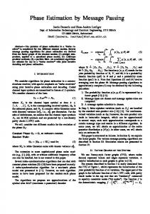
Fig. 1. Comparison of the least squares range estimator with wavelengths A (top) and C (bottom) suitable for the basis in [10] and B (top) and D (bottom) suitable only for the basis described in this paper. Sets B and D result in smaller mean square error when the noise variance σ2 is greater than approximately 1.2 × 10⁻⁴ and 7 × 10⁻⁵ respectively.
That U is unimodular follows immediately from the unimodularity of A1 , . . . , AN −1 . It remains to show that the first column of U is equal to v. Let v1 , . . . , vN −1 be column vectors of length N defined as vk = (v1 , . . . , vk , gk+1 , 0, . . . , 0)′ ,
k = 1, . . . , N − 2
′
vN −1 = (v1 , . . . , vN −1 , gN ) = v. One can readily check that vk+1 = Ak+1 vk for all k = 1, . . . , N − 1. The first column of the matrix A Q1Kis v1 and so, by induction, the first column of the product k=1 Ak is vK for all K = 1, . . . , N − 1. It follows that the first column of U is vN −1 = v as required. Let U2 be the N by N − 1 matrix formed by removing the first column from U, that is, U2 = (u2 , . . . , uN ). By Proposition 2 a basis for Λ∗ is given by projecting the columns of U2 orthogonally to v, that is, a basis matrix for Λ∗ is the N by N − 1 matrix B = QU2 . Given B a general purpose ˆ ∈ ZN −1 such that algorithm [14] can be used to compute w ∗ ˆ = Bw ˆ is a closest lattice point in Λ to Qy ∈ RN . Now x ˆ = Qˆ ˆ = Bw ˆ = QU2 w z x ˆ ∈ ZN . The least squares range estimator rˆ and so zˆ = U2 w is then given by (6).
For both sets the wavelengths are contained in the interval [2, 7] and P = 210 = lcm(A) = lcm(B) so that the identifiable range is the same. The wavelengths A are relatively prime integers and are suitable for the basis of Li et. al. [10] and are used in the simulations in [10]. The wavelengths B are not suitable for the basis of [10] because they can not be scaled to pairwise relatively prime integers. To see this, observe that the smallest positive number by which we can multiply the elements of B to obtain integers is c = 6124949 210 . Multiplying the elements of B by c we obtain the set c × B = {77531, 100409, 149389, 197579} and these elements are not pairwise relatively prime because, for example, gcd(77531, 100409) = 1271. Figure 1 shows the results of simulations with both sets A and B. When the noise variance σ 2 is small wavelengths A result in slightly reduced sample mean square error as compared with B. As σ 2 increases the sample mean square error exhibits a ‘threshold’ effect and increases suddenly. The threshold occurs at σ 2 ≈ 1.2 × 10⁻⁴ for wavelengths A and σ 2 ≈ 3 × 10⁻⁴ for wavelength B. Wavelengths B are more accurate than A when σ 2 is greater than approximately 1.2 × 10⁻⁴ . For N = 5 the two sets of wavelengths are 2310 2310 2310 2310 C = {2, 3, 5, 7, 11}, D = { 2310 877 , 523 , 277 , 221 , 211 }.
For both sets all wavelengths are contained in the interval [2, 11] and P = 2310 = lcm(C) = lcm(D) so that the maximum identifiable range is the same. The basis of Li et. al. [10] can be used for wavelengths C but not for D. The wavelengths C were used in the simulations in [10]. Figure 1 shows the result of Monte-Carlo simulations with these wavelengths. Wavelengths C result in slightly smaller sampler mean square error than D when σ 2 is small, but dramatically more error for σ 2 above the threshold occurring at σ 2 ≈ 7 × 10⁻⁵ . The sets B and D have been selected based on a heuristic optimisation criterion. The properties of this criterion are not yet fully understood and will be the subject of a future paper.
V. S IMULATION R ESULTS We present the results of Monte-Carlo simulations with the least squares range estimator. Simulations with N = 4 and N = 5 wavelengths are performed. For each case we consider two different set of wavelengths. The first set is suitable for the basis of Li et. al. [10] and was used in the simulations in [10]. The second set is suitable only for our basis. In each simulation the true range r0 = 20 and the phase noise variables Φ1 , . . . , ΦN are wrapped normally distributed, that is, Φn = hXn i where X1 , . . . , XN are independent and normally distributed with zero mean and variance σ 2 . In this case, the least squares estimator is also the maximum likelihood estimator. Figure 1 shows the sample mean square
VI. C ONCLUSION We have considered least squares/maximum likelihood estimation of range from observation of phase at multiple wavelengths. The estimator can be computed by finding a closest point in a lattice. This requires a basis for the lattice. Bases have previously been constructed under the assumption that the wavelengths can be scaled to relatively prime integers. In this paper, we gave a construction in the general case and indicated by simulation that this can dramatically improve range estimates. An open problem is how to select wavelengths to maximise the accuracy of the least squares estimator. We will study this problem in future research.
5
R EFERENCES [1] E. Jacobs and E.W. Ralston, “Ambiguity resolution in interferometry,” IEEE Trans. Aerospace Elec. Systems, vol. 17, no. 6, pp. 766–780, Nov. 1981. [2] J. M. M. Anderson, J. M. Anderson, and E. M. Mikhail, Surveying, theory and practice, WCB/McGraw-Hill, 1998. [3] P. J. G. Teunissen, “The LAMBDA method for the GNSS compass,” Artificial Satellites, vol. 41, no. 3, pp. 89–103, 2006. [4] P. J. G. Teunissen, “The least-squares ambiguity decorrelation adjustment: a method for fast GPS integer ambiguity estimation,” Journal of Geodesy, vol. 70, pp. 65–82, 1995. [5] S. D. Chitte, S. Dasgupta, and D. Zhi, “Distance estimation from received signal strength under log-normal shadowing: Bias and variance,” IEEE Signal Process. Letters, vol. 16, no. 3, pp. 216–218, March 2009. [6] H.-C. So and L. Lin, “Linear least squares approach for accurate received signal strength based source localization.,” IEEE Trans. Sig. Process., vol. 59, no. 8, pp. 4035–4040, 2011. [7] X. Li and K. Pahlavan, “Super-resolution TOA estimation with diversity for indoor geolocation,” IEEE Trans. Wireless Commun., vol. 3, no. 1, pp. 224–234, Jan 2004. [8] S. Lanzisera, D. Zats, and K.S.J. Pister, “Radio frequency timeof-flight distance measurement for low-cost wireless sensor localization,” IEEE Sensors Journal, vol. 11, no. 3, pp. 837– 845, March 2011. [9] C. E. Towers, D. P. Towers, and J. D. C. Jones, “Optimum frequency selection in multifrequency interferometry,” Optics Letters, vol. 28, pp. 887–889, 2003. [10] W. Li, X. Wang, X. Wang, and B. Moran, “Distance estimation using wrapped phase measurements in noise,” IEEE Trans. Sig. Process., vol. 61, no. 7, pp. 1676–1688, 2013. [11] D. Odijk, P. Teunissen, and B. Zhang, “Single-frequency integer ambiguity resolution enabled GPS precise point positioning,” J. of Surveying Eng., vol. 138, no. 4, pp. 193–202, 2012. [12] A. Hassibi and S. P. Boyd, “Integer parameter estimation in linear models with applications to gps,” IEEE Trans. Sig. Process., vol. 46, no. 11, pp. 2938–2952, Nov 1998. [13] L. Babai, “On Lov´asz lattice reduction and the nearest lattice point problem,” Combinatorica, vol. 6, pp. 1–13, 1986. [14] E. Agrell, T. Eriksson, A. Vardy, and K. Zeger, “Closest point search in lattices,” IEEE Trans. Inform. Theory, vol. 48, no. 8, pp. 2201–2214, Aug. 2002. [15] K. V. Mardia and P. Jupp, Directional Statistics, John Wiley & Sons, 2nd edition, 2000. [16] R. G. McKilliam, Lattice theory, circular statistics and polynomial phase signals, Ph.D. thesis, University of Queensland, Australia, December 2010. [17] N. I. Fisher, Statistical analysis of circular data, Cambridge University Press, 1993. [18] J. Martinet, Perfect lattices in Euclidean spaces, Springer, 2003. [19] D. Micciancio, “The hardness of the closest vector problem with preprocessing,” IEEE Trans. Inform. Theory, vol. 47, no. 3, pp. 1212–1215, 2001. [20] J. Jalden and B. Ottersten, “On the complexity of sphere decoding in digital communications,” IEEE Trans. Sig. Process., vol. 53, no. 4, pp. 1474–1484, April 2005. [21] R. Kannan, “Minkowski’s convex body theorem and integer programming,” Math. Operations Research, vol. 12, no. 3, pp. 415–440, 1987. [22] C. P. Schnorr and M. Euchner, “Lattice basis reduction: Improved practical algorithms and solving subset sum problems,” Math. Programming, vol. 66, pp. 181–191, 1994. [23] E. Viterbo and J. Boutros, “A universal lattice code decoder for fading channels,” IEEE Trans. Inform. Theory, vol. 45, no. 5, pp. 1639–1642, Jul. 1999. [24] D. Micciancio and P. Voulgaris, “A deterministic single exponential time algorithm for most lattice problems based on Voronoi cell computations,” SIAM Journal on Computing, vol. 42, no. 3, pp. 1364–1391, 2013.
[25] R. G. McKilliam, W. D. Smith, and I. V. L. Clarkson, “Lineartime nearest point algorithms for Coxeter lattices,” IEEE Trans. Inform. Theory, vol. 56, no. 3, pp. 1015–1022, Mar. 2010. [26] R. McKilliam, A. Grant, and I. Clarkson, “Finding a closest point in a lattice of Voronoi’s first kind,” SIAM Journal on Discrete Mathematics, vol. 28, no. 3, pp. 1405–1422, 2014. [27] R. G. McKilliam, B. G. Quinn, I. V. L. Clarkson, and B. Moran, “Frequency estimation by phase unwrapping,” IEEE Trans. Sig. Process., vol. 58, no. 6, pp. 2953–2963, June 2010. [28] R. G. McKilliam, B. G. Quinn, and I. V. L. Clarkson, “Direction estimation by minimum squared arc length,” IEEE Trans. Sig. Process., vol. 60, no. 5, pp. 2115–2124, May 2012. [29] R.G. McKilliam, B.G. Quinn, I.V.L. Clarkson, B. Moran, and B.N. Vellambi, “Polynomial phase estimation by least squares phase unwrapping,” IEEE Transactions on Signal Processing, vol. 62, no. 8, pp. 1962–1975, April 2014. [30] M. Pohst, “A modification of the LLL reduction algorithm,” J. Symbolic Computation, , no. 4, pp. 123–127, 1987.