is repeated for 6 combinations of Eact and Kact. (see Table 2). All the configurations are run with ε = 1% for all the responses. 4.3 Fidelity map and likelihoods.
Bayesian Calibration Using Fidelity Maps Sylvain Lacaze & Samy Missoum Aerospace and Mechanical Engineering Department, University of Arizona, Tucson, Arizona, 85721
ABSTRACT: This paper introduces a new approach for model calibration based on fidelity maps. Fidelity maps refer to the regions of the parameter space within which the discrepancy between computational and experimental data is below a user-defined threshold. It is shown that fidelity maps, which are built explicilty in terms of the calibration parameters and aleatory variables, provide a rigourous approximation of the likelihood for maximum likelihood estimation or Bayesian update. Because the maps are constructed using a support vector machine classifier (SVM), the approach has the advantage of handling numerous correlated responses, possibly discontinuous, at a moderate computational cost. This is made possible by the use of a dedicated adaptive sampling scheme to refine the SVM classifier. A simply supported plate with uncertainties in the boundary conditions is used to demonstrate the methodology. In this example, the construction of the map and the Bayesian calibration is based on several natural frequencies and mode shapes to be matched simultaneously.
1 INTRODUCTION Computational models are used to predict the static or dynamic behavior of structures. However, there might be marked discrepancies between the prediction of the model and experimental data. In order to reduce this difference, the model might need to be calibrated (or updated) by searching the values of parameters (e.g., material properties) that best “match” the data. For instance, in modal analysis, the characteristics of the model (e.g., stiffness and mass distribution) will be modified so as to match experimental natural frequencies and mode shapes (Marwala 2010). The most widely used approach in engineering applications is the least square approach. However, because uncertainties might have a pronounced effect on the responses of the system, this approach, often implemented in a deterministic way, is in general not suitable (Chen, Duhamel, & Soize 2006, Gogu, Haftka, Le Riche, Molimard, Vautrin, et al. 2010). For this reason, statistical approaches have been favored to extract distributions of update parameters and responses. The two most common statistical approaches are the maximum likelihood estimate and Bayesian update. While the maximum likelihood approach (Pratt 1976, Aldrich 1997) finds the most “probable” values of the parameters to be estimated, the Bayesian method (Press & Press 1989, Carlin
& Louis 1997) focuses on refining the parameter distributions inferred from previous knowledge. The implementation of these approaches, which both require the assessment of the likelihood, is severely hampered by difficulties such as the large computational time per simulation and the inclusion of both aleatory and epistemic uncertainties. In addition existing approaches are not able to handle a large number of responses to match without making restrictive independence assumptions. Further difficulties appear in the case of discontinuous responses. The proposed update approach is designed to provide a flexible scheme which tackles the aforementioned technical difficulties such as the inclusion of a large number of correlated responses, the computational time, and discontinuities. This work is based on the construction of the explicit boundary of the region of the parameter space where the discrepancy between model and experiments is below a given threshold. This domain is referred to as “fidelity map” and can be shown to provide a rigorous and efficient approximation of the likelihood. The boundaries are constructed using a Support Vector machine (SVM) which is a classification technique used to explicitly separate data belonging to two classes (Gunn 1998, Vapnik 2000,
Christianini & Taylor 2000, Sch¨olkopf & Smola 2002). All the computational cost is therefore concentrated within the construction of the boundary while the likelihood can be approximated from the fidelity map. The main advantages of the approach stems from the classification paradigm which allows one to manage a large number of (potentially discontinuous) responses simultaneously. This article is constructed as follows. Section 2 provides the notation and the general idea of the proposed work. Section 3 describes the computation of the likelihood and posterior distribution for a given fidelity map. Section 3.1 provides a background on SVM and Section 3.2 on the adaptive sampling to accurately build the SVM. Finally, Section 4 will present results for a demonstrative example of a plate with uncertainty on the boundary conditions. 2 ILLUSTRATIVE EXAMPLE AND NOTATIONS
As an illustrative example, consider a model in the form of a cantilever column (e.g., representative of a building) with wind load (Figure 1(a)). In this toy example, we wish to estimate the bending stiffness of the column K ≡ X based on a set of experimental data y exp (e.g., deflection δ) knowing that the the column is subjected to a random load F ≡ A with known probabilistic distribution.
δ
Likelihood
X
X
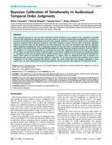
Figure 2: The fidelity map is then used to build an approximation of the likelihood.
Figure 1(b) depicts the construction of the fidelity map corresponding to p experiments and n responses (e.g., displacements, accelerations etc.) per experiment. The fidelity map, constructed accurately with a support vector machine classifier and adaptive sampling (see Section 3), provides the region of the space where the relative discrepancy between model and experiments ∆f i is lower than 1% for every response. This allows the update of the model through maximum likelihood or Bayesian update.
A fidelity map is defined as the region of the parameter space within which the responses belong to a user-defined interval around the experimental data: F M = {(x, a) | ri (x, a) ≤ εi , i = 1, . . . , n}
(1)
where: yi (x, a) − yiexp ri (x, a) = yiexp Using the fidelity map, it can be shown (see Section 3.3) that the likelihood can be efficiently approximated (cf. Figure 2). 3.1 SVM-based fidelity map Fidelity maps are constructed using a support vector machine (SVM) classifier. An SVM defines the boundaries between samples of two different classes (e.g., feasible and infeasible) (Gunn 1998, Vapnik 2000, Sch¨olkopf & Smola 2002, Christianini & Taylor 2000). In the context of fidelity maps, SVM has the following advantages:
p experiments F
K
max ri < εi
3 FIDELITY MAPS AND CONSTRUCTION OF THE LIKELIHOOD
Consider the responses y of a model and the corresponding experimental measurements yexp . The responses of the system are governed by two types of inputs: the first set are the parameters to estimate X (e.g., material property) while the second one, A, will be referred to as “aleatory” parameters. The probability density function (PDF) of a random variable X is noted fX and its cumulative distribution function (CDF) is noted FX .
F
A
• Only one SVM decision function is needed irrespective of the number n of responses y;
n responses ∆δi < 1% K
(a) Model.
(b) Fidelity map.
Figure 1: Illustrative example. Calibration of the stiffness K of a column subjected to a random (aleatory) load F based on experimental responses.
• It is insensitive to discontinuities and can handle binary responses (Basudhar, Missoum, & Harrison Sanchez 2008); • The boundaries can be highly nonlinear and correspond to disjoint non-convex domains;
• The prediction of a class is very efficient, thus allowing the use of Monte-Carlo type sampling. Given N training sample, the SVM classifier is expressed as: s(x) = b +
N X
λ(k) l(k) K(x(k) , x)
(2)
k=1
3.2.2 Adaptive sampling In order to build an accurate SVM at affordable cost, Basudhar and Missoum introduced an adaptive sampling scheme that is used in this work. Assuming the existence of at least one point within the fidelity map (c.f. Section 3.2.1), the SVM can be refined using the following two types of samples (c.f. Basudhar & Missoum 2008, Basudhar & Missoum 2010 for details):
where x(k) is the k th training sample, λ(k) is the corresponding Lagrange multiplier, l(k) is the label (class) that can take values +1 or -1, K is a kernel function (e.g. Gaussian in this work) and b is the bias. The boundary is then defined as s(x) = 0.
A primary sample Also referred as “maxmin” sample. This sample is defined as the point in the space that maximizes the minimum distance to existing samples (i.e., sparse regions) under the constraint that it lies on the SVM boundary (i.e., s(x)=0).
In order to build the fidelity map, an SVM is initially trained using a design of experiments (DOE). The class of each sample is defined based on the discrepancy between the model outputs and the experimental measurements. To be feasible, a training sample must correspond to absolute relative differences ri between the model outputs yi and the measurements yiexp less than a given threshold εi (i.e., issue outputs lying within a “confidence region”). Therefore, the labels used to train the SVM are defined as: � (k) (k) l = +1 if ri ≤ εi , i = 1, . . . , n −1 otherwise
A secondary sample is used to prevent a phenomenon referred as “locking” of the SVM, where adding primary samples only generates small changes of the boundary. For this reason, this sample is also referred to as “antilocking” sample.
where: y (k) − y exp (k) ri = i exp i yi 3.2 Map refinement and adaptive sampling In order for the likelihood to be accurate, a small enough ε is needed as well as an accurate boundary. 3.2.1 Notion of most “feasible” sample It might happen that in the initial DOE there is not a single sample that satisfies the initial fidelity requirement imposed by the various (small) εi . Therefore no feasible sample is available to construct an SVM. In order to solve this issue, the sample x(kc ) with the minimum discrepancy over all the responses is searched. The index kc of the most “feasible sample” is: (k) kc = arg min rmax
(3)
k
where: (k)
(k) rmax = max i
ri − εi εi
!
The sampling schedule used in this work uses two primary samples and one secondary sample per iteration (Basudhar & Missoum 2010). Algorithm 1, summarizes the construction of the fidelity map. Algorithm 1 Fidelity map. Adaptive Sampling. Require: User define how small the fidelity map must be by setting ε; 1: Sample the space ({X, A}) according to a DOE of size np (here, CVT) : w(k) = [x(k) , a(k) ]; 2: Evaluate all samples : y(k) = y(w(k) ); 3: Define the scaled residual relative to each mea yexp −y(k) (k) surements for all points : ri = i yexp i ; i 4: For each point, define � � their “feasibility” : (k)
rmax = maxi
(k)
ri −εi εi
;
Begin adaptive sampling: for j = np + 1 → np + nadapt do ; Set labels ton-1: l(k) = −1, o k = 1, . . . , j − 1; (k) 8: Define K = k|rmax ≤ 0 ; 9: if K = ∅ then; (l) 10: Find kc = arg min rmax ; 5: 6: 7:
l
Define K = {kc }; end if Set l(k) = +1 ∀k ∈ K; Build the SVM as explained in Section 3.1; Add an adaptive sample w(j) as explain in Section 3.2.2; (j) 16: Compute : y(j) , r(j) , rmax ; 17: end for
11: 12: 13: 14: 15:
3.3 Likelihood approximation This section shows how to relate the fidelity map to the likelihood. It can be shown that as the εi tend to zero, the likelihood can be obtained. This can be proven, without loss of generality and for the sake of simplicity, with x and y exp as two scalars. The relation between a PDF and a CDF is given as: fY (x,A) (y exp |x) =
dFY (x,A) exp (y |x) dy
Therefore: fY (x,A) (y exp |x) = P[y exp − ε ≤ Y (x, A) ≤ y exp + ε|x] ε→0 2ε exp The probability P[y − ε ≤ Y (x, A) ≤ y exp + ε|x] is the probability of the responses to lie within the user-defined intervals around the experimental results knowing x. Follows the important result: lim
fY (x,A) (y exp |x) ∝ ∼ P [(x, A) ∈ F M ]
(4)
where ∝ ∼ stems for “approximately proportional to”. This probability can be efficiently estimated using Monte Carlo sampling over the aleatory variables. As ε tends to zero, this probability tends to the likelihood value. 3.4 Estimation based on the approximated likelihood 3.4.1 Maximum Likelihood Estimate Once the fidelity map is constructed, maximum likelihood estimates (MLE) (Xiong, Chen, Tsui, & Apley 2009) can be obtained: xM LE = argmax fY(x,A) (yexp |x)
(5)
where fX (x|yexp ) is the posterior distribution, fY(x,A) (yexp |x) is the likelihood, fX (x) is the prior knowledge, and fY(X,A) (yexp ) is a normalizing constant which represent the overall probability density to observe yexp . In order to sample the posterior distribution, a Markov Chain Monte Carlo algorithm such as the Metropolis-Hastings algorithm (Metropolis, Rosenbluth, Rosenbluth, & Teller 1953, Hastings 1970) can be used to overcome the difficulty of evaluating fY(X,A) (yexp ). Instead of an MLE estimate, one can now use a Bayes estimator defined as the expectation of the posterior distribution: Z Bayes exp xi = E [Xi |y ] = xi fX (x|yexp )dx (7) In order to assess the refinement in the fidelity of the model, in a statistical sense, using the posterior in comparison to the prior, the following fidelity index can be estimated: FI =
P[(X, A) ∈ F M |yexp ] P[(X, A) ∈ F M ]
(8)
where P[(X, A) ∈ F M |yexp ] (resp. P[(X, A) ∈ F M ]) is computed using the posterior distribution fX (x|yexp ) (resp. the prior distribution fX (x)). 4 RESULTS The proposed methodology is applied to the update of a finite element (FE) dynamic model based on modal properties. Model parameter estimation using natural frequencies and mode shapes is a typical example where the number of outputs y is rather high (Allemang 2002, Chen, Duhamel, & Soize 2006, Marwala 2010, Gogu, Haftka, Le Riche, Molimard, Vautrin, et al. 2010).
As mentioned previously, this approach provides a point estimate xest . In order to obtain a distribution of the estimated parameters and have a fully stochastic approach, one can use the Bayesian approach.
The test example used is a simple plate subjected to uncertainty in the boundary conditions. We wish to identify the Young’s modulus given a set of natural frequencies and mode shapes. For comparison purposes, the results are performed along with an approach based on a residual. It is also compared to the product of the individual likelihoods corresponding to the various responses (See Appendix A). The product of likelihoods is used in order to show the influence of correlated model outputs.
3.4.2 Bayesian Estimate Starting with the Bayes formula:
4.1 Finite element Model updating based on modal data
fA|B fB = fB|A fA
Traditional quantities used in model update using modal properties are:
x
At this point it is essential to note that the dependence between the responses is implicitly accounted for.
and specializing it to model update, we obtain: fY(x,A) (yexp |x)fX (x) fX (x|yexp ) = fY(X,A) (yexp )
(6)
• Differences in natural frequencies values (e.g., Euclidean norm of difference). This quantity is traditionally minimized in the form
Table 1: Parameters used for the plate example (S.I. units).
Deterministic To estimate Aleatory Parameter a b ν ρ t E K Value, Distribution 1 1.5 0.33 7800 0.01 N/A U (2 × 10⁵ , 106 ) of a residual through optimization. Various weights can be assigned to the different frequencies if more emphasis is to be given to particular ones; • Differences between the mode shapes. This is typically measured using the Modal Assurance Criterion (MAC) matrix (c.f. Eq. 9); • Differences between the Frequency Response Function (FRFs) measured using the FRAC (Frequency Response Assurance Criterion);
a
b E, ν, ρ, t K
(a) Schematic representation.
(b) FEM representation.
Figure 3: Schematic and Finite Element representation of a simple plate. One side is simply supported while the others are connected to the ground through springs, to model uncertainties in the boundary conditions.
• Mode orthogonality. The “MAC” criterion (Allemang 2002, Marwala 2010) is by far the most widely used: Mij =
2 (Φ∗T i AΦexp,j ) ∗T (Φ∗T i AΦi )(Φexp,j AΦexp,j )
(9)
where Φi is the ith computational mode shape and is the conju“exp” stands for experimental. Φ∗T i gate transpose of the mode shape. A is often the identity matrix or the mass matrix. The MAC value is equal to unity for a perfect match of modes. It should be as close to zero as possible for cross terms. 4.2 Simply supported plate As an example, we consider a rectangular plate. The plate is simply supported. In order to model the uncertainties in the displacement boundary conditions, one dimensional springs of stiffness K are used for three sides of the plate (Figure 3). The finite element model of the plate is constructed with 80 shell elements. We wish to identify the Young’s modulus E of the plate based on Nm = 4 first modes for a total of n = 14 responses. The parameters are summarized in Table 1. In order to define the “experiments”, the FE model is run with E = Eact and K = Kact . The methodology is repeated for 6 combinations of Eact and Kact (see Table 2). All the configurations are run with ε = 1% for all the responses.
(i.e., the approximated likelihood noted LHmcs ) is calculated with 105 Monte Carlo samples according to the distribution of K. The proposed approach is compared to the results using the likelihood of the residual (LHres ) and the product of the likelihoods for the different responses LHprod (see Appendix A). These likelihoods are constructed using Kernel Smoothing (Bowman & Azzalini 1997) and Kriging models(Sacks, Welch, Mitchell, & Wynn 1989, Jones 2001, Forrester & Keane 2009, Basudhar, Dribusch, Lacaze, & Missoum 2012) trained with 65 CVT samples. LHres uses a residual defined as follows (Appendix A): " # Nm Nm 2 X X (λi − λexp ) i R= + (Mii − 1)2 + Mij exp λ i i=1 j=i+1 The graphical results for 2 cases are depicted on Figure 4. Graphical inspection of the likelihoods show that LHmcs exhibits a higher robustness than the two other methods for that example. The failure of the LHprod is natural since the different natural frequencies are strongly correlated, therefore, the assumption of independence leads to incorrect results. On the other hand, the inaccuracy of LHres is not straightforward. A loose explanation stems from the gathering of several responses that are correlated with different spreads within one quantity (similar to conclusion drawn in Gogu, Haftka, Le Riche, Molimard, Vautrin, et al. 2010).
4.3 Fidelity map and likelihoods The fidelity map is constructed in the (E, K) space with 15 Central Voronoi Tessellation (CVT) samples. The boundary is then refined with 50 additional adaptive samples. For each value of E, the probability of being within the fidelity map
4.4 Maximum likelihood estimate In the case where MLE is chosen for estimation, the results for the six cases are summarized in Table 2. As can be seen, the methodology is robust for this example.
5
x 10
1
10
SVM Positive samples Negative Samples
9
LHmcs LHres LHprod Eact
0.9 0.8
8
0.7 0.6
LH
K (N/m)
7
6
0.5 0.4
5
0.3 4
0.2 3
0.1 0 1.2
2 1.4
1.6
1.8
2
2.2
2.4
2.6
E (P a)
2.8
1.4
1.6
1.8
2
2.2
2.4
2.6
2.8
E (P a)
11
x 10
(a) SVM process
3 11
x 10
(b) Likelihood
5
x 10
1
10
SVM Positive samples Negative Samples
9
LHmcs LHres LHprod Eact
0.9 0.8
8
0.7 0.6
LH
K (N/m)
7
6
0.5 0.4
5
0.3 4
0.2 3
0.1 0 1.2
2 1.4
1.6
1.8
2
2.2
2.4
2.6
E (P a)
2.8
1.4
1.6
1.8
2
2.2
E (P a)
11
x 10
(c) SVM process
2.4
2.6
2.8
3 11
x 10
(d) Likelihood
Figure 4: Graphical results of the plate example, showing the fidelity maps and the estimated likelihoods, for Eact = 185 × 109 P a and Kact = 3 × 10⁵ N.m−1 (a and b) and Eact = 235 × 109 P a and Kact = 6 × 10⁵ N.m−1 (c and d).
Table 2: Summary of the 6 experimental configurations and Figures associated (S.I. units).
185 × 109
Eact
235 × 109
Kact
3 × 10⁵
6 × 10⁵
9 × 10⁵
3 × 10⁵
6 × 10⁵
9 × 10⁵
Figures
4(a) & 4(b)
N\a
N\a
N\a
4(c) & 4(d)
N\a
M LE Eest (P a)
184.6 × 10⁹
182.3 × 10⁹
185.8 × 10⁹
232.4 × 10⁹
237.5 × 10⁹
235.4 × 10⁹
Error (%)
0.22
1.46
0.49
1.11
1.06
0.17
Bayes Eest (P a)
184.3 × 10⁹
185.02 × 10⁹
186.7 × 10⁹
233.9 × 10⁹
233.7 × 10⁹
235.5 × 10⁹
Error (%)
0.37
0.008
0.87
0.44
0.54
0.19
4.5 Bayesian update
5
4
In the case of Bayesian update, a wide prior, reflecting a substantial lack of knowledge was chosen. The prior is set with a mean value of 210 GP a and a standard deviation of 21 GP a. Figure 5(a) depicts the likelihood function, the prior distribution and the actual value, for the first case (Eact = 185 × 109 P a and Kact = 3 × 10⁵ N.m−1 ). Figure 5(b) shows the corresponding posterior distribution (Section 3.4.2). The Bayes estimators for the 6 cases are shown in Table 2. As an example of improvement brought by the Bayesian update in comparison to MLE, the fidelity index was computed for one case (Eact = 185 × 109 P a and Kact = 3 × 10⁵ N.m−1 ). A large value of 8.23 was obtained indicating that the posterior distribution gives roughly 8 times more chances to match the measurements. In order to further gauge the benefits of the Bayesian update, the posterior was propagated to the first natural frequency (Figure 6(a)). For comparison, the prior was also propagated (Figure 6(b)). In addition the ideal, unknown, response distribution was computed (Figure 6(c)) using the actual value of the Young’s modulus (Eact ) along with the propagation of the aleatory variables (i.e. K). The distribution of the first natural frequency clearly shows that the benefits of the Bayesian update.
5
5
x 10
3.5
x 10
2.5
3
3
x 10
2
2.5 1.5
2
2 1.5
1
1
1
0.5
0.5
0
25
30
35
40
λ1 (H z)
(a) Prior propagation.
0
25
30
35
λ1 (H z)
(b) Ideal propagation.
40
0
25
30
35
40
λ1 (H z)
(c) Posterior propagation.
Figure 6: Propagations of the uncertainties applied to the first natural frequency of the first configuration (Eact = 185 × 109 P a and Kact = 3 × 10⁵ N.m−1 ) of the plate example.
uncertainties, allow one to efficiently approximate the likelihood with Monte-Carlo simulations. In order to obtain an accurate boundary and reduce the number of model calls, an adaptive sampling scheme is used. Because SVM is a classification method, a large number of correlated model outputs can be used. Finally, this approach do not rely on any assumption, except a user define vector of variables, ε. The next steps of this research will study the scalability of the approach in higher dimensions. In addition, the approach will be tested on real world problems with actual experiments. 6 ACKNOWLEDGMENTS
1
LHmcs Eact Prior
0.9 0.8
1 0.9
Support from the National Science Foundation (award CMMI-1029257) is gratefully acknowledged.
0.8
0.7 0.7
LH
MCMC
0.6 0.5 0.4
0.6 0.5 0.4
0.3
0.3
0.2
0.2
0.1
0.1
0 1.5
2
2.5
E (P a)
3 11
x 10
(a) Plot of the likelihood function, prior knwoledge and actual value.
REFERENCES
0 1.5
2
2.5
E (P a)
3 11
x 10
(b) MCMC samples.
Figure 5: Bayesian process applied to the first case (Eact = 185 × 109 P a and Kact = 3 × 10⁵ N.m−1 ) of the plate example.
5 CONCLUSION An approach to perform model update using fidelity maps has been introduced. The construction of explicit fidelity maps using SVM in a space with parameter to estimate and aleatory
Aldrich, J. (1997). Ra fisher and the making of maximum likelihood 1912-1922. Statistical Science 12 (3), 162–176. Allemang, R. (2002). The modal assurance criterion (mac): twenty years of use and abuse. In Proceedings, International Modal Analysis Conference. Basudhar, A., C. Dribusch, S. Lacaze, & S. Missoum (2012). Constrained efficient global optimization with support vector machines. Structural and Multidisciplinary Optimization, 1–21. Basudhar, A. & S. Missoum (2008). Adaptive explicit decision functions for probabilistic design and optimization using support vector machines. Computers & Structures 86 (19-20), 1904–1917. Basudhar, A. & S. Missoum (2010). An improved adaptive sampling scheme for the construction of explicit boundaries. Structural and Multidisciplinary Optimization 42 (4), 517–529. Basudhar, A., S. Missoum, & A. Harrison Sanchez (2008). Limit state function identification using support vector machines for discontinuous responses and disjoint failure domains. Probabilistic Engineering Mechanics 23 (1), 1– 11.
Bowman, A. & A. Azzalini (1997). Applied smoothing techniques for data analysis: the kernel approach with S-Plus illustrations, Volume 18. Oxford University Press, USA. Carlin, B. & T. Louis (1997). Bayes and empirical Bayes methods for data analysis, Volume 7. Springer. Chen, C., D. Duhamel, & C. Soize (2006). Probabilistic approach for model and data uncertainties and its experimental identification in structural dynamics: Case of composite sandwich panels. Journal of Sound and vibration 294 (1), 64–81. Christianini, N. & S. Taylor (2000). An introduction to support vector machines (and othre kernel-based learning methods). Forrester, A. & A. Keane (2009). Recent advances in surrogate-based optimization. Progress in Aerospace Sciences 45 (1-3), 50–79. Gogu, C., R. Haftka, R. Le Riche, J. Molimard, A. Vautrin, et al. (2010). Introduction to the bayesian approach applied to elastic constants identification. AIAA journal 48 (5), 893–903. Gunn, S. (1998). Support vector machines for classification and regression. ISIS technical report 14. Hastings, W. (1970). Monte carlo sampling methods using markov chains and their applications. Biometrika 57 (1), 97–97. Jones, D. (2001). A taxonomy of global optimization methods based on response surfaces. Journal of Global Optimization 21 (4), 345–383. Marwala, T. (2010). Finite Element Model Updating Using Computational Intelligence Techniques: Applications to Structural Dynamics. Springer. Metropolis, N., A. W. Rosenbluth, M. N. Rosenbluth, & A. H. Teller (1953). Equation of state calculations by fast computing machines. The Journal of Chemical Physics 21 (6), 1087–1092. Pratt, J. (1976). Fy edgeworth and ra fisher on the efficiency of maximum likelihood estimation. The Annals of Statistics 4 (3), 501–514. Press, S. & J. Press (1989). Bayesian statistics: principles, models, and applications. Wiley New York. Sacks, J., W. Welch, T. Mitchell, & H. Wynn (1989). Design and analysis of computer experiments. Statistical science 4 (4), 409–423. Sch¨ olkopf, B. & A. Smola (2002). Learning with kernels: Support vector machines, regularization, optimization, and beyond. the MIT Press. Vapnik, V. (2000). The nature of statistical learning theory. Springer Verlag. Xiong, Y., W. Chen, K. Tsui, & D. Apley (2009). A better understanding of model updating strategies in validating engineering models. Computer Methods in Applied Mechanics and Engineering 198 (15-16), 1327–1337.
A PRODUCT OF THE LIKELIHOODS AND RESIDUAL For comparison with the proposed approach, this appendix introduces two other methods to perform a scalable likelihood computation. These two approaches are used in the result section 4.
A.1 Product of the likelihoods If one assumes n responses to be independent (an obviously wrong assumption!), the likelihood is the
product of the individual likelihoods: x
MLE
= argmax x
n Y
fYi (x,A) (yiexp |x)
(10)
i=1
A.2 A Residual-based likelihood A seemingly intuitive approach is to use a residual that combines n responses into one quantity: R(x, a) =
�2 n � exp X y − yi (x, a) i
i=1
yiexp
(11)
A possible MLE then reads: xMLE = argmax fR(x,A) (0|x)
(12)
x
It is noteworthy to mention that this method does not compute exactly the likelihood as demonstrated in the results section.