Bayesian inference in hidden Markov random fields for binary data defined on large lattices N. Friel† University of Glasgow, UK
A.N. Pettitt Queensland University of technology, Australia
R. Reeves Queensland University of technology, Australia
E. Wit University of Glasgow, UK Summary. A hidden Markov random fields may arise where a Markov random field – a spatial arrangement of correlated discrete states – is corrupted by some observational noise process. We assume that the number of hidden or latent states is known and wish to perform inference on all unknown parameters. The main challenge in such cases is to calculate the likehood of the hidden states, which could be computationally very expensive. Recently new methods have been proposed to circumvent this problem, all of which are restricted to relatively small lattices. The main contribution of this paper is to introduce approximate methods to compute the likelihood for large lattices based on exact likelihood calculations for smaller lattices. We introduce approximate likelihood methods by relaxing some of the dependencies in the latent model, and also by approximating the likelihood by a partially ordered Markov model defined on a collection of sublattices. Results are presented based on simulated data as well as inference for the temporal-spatial structure of the interaction between up- and down-regulated states within the mitochondrial chromosome of the Plasmodium falciparum organism. Keywords: Markov random fields; Autologistic model; Ising model; Latent variables; Markov chain Monte Carlo methods; Normalising constant
1. Introduction This paper is concerned with the problem of carrying out inference for a hidden Markov random field model. This is an example of a general statistical problem of the following type: observed data y masks or hides some unobserved latent or missing process x. Denote all model parameters by θ. Interest may be in inference about parameters θ, or about about the latent or missing data x. The posterior distribution for θ, p(θ|y), is often intractable, but computation can often be simplified by including the hidden or missing data x in the inference procedure. That is, by examining the posterior distribution p(θ, x|y). A standard Bayesian analysis might then proceed by iteratively updating beliefs about θ and x in turn. Widely studied examples of this set-up include mixture models and hidden Markov models. In this paper we consider the situation where the latent hidden variable x takes the form of a Markov random field (MRF). This problem is thus seen as one of performing inference for a hierarchical model, or more generally a directed graphical model, where a hyperprior is placed on the distribution of the hidden MRF. An early analysis of this type of problem appeared in (Besag et al 1991). In fact the hugely influential work of Geman and Geman (1984) examined a similar problem in image analysis, but where the hidden Ising model had a known parameter value. A major difficulty with this type of problem is that the likelihood p(x|θ) of the hidden layer given the model parameters is often intractable, due to the difficulty of calculating its normalising constant. To circumvent this intractability Besag et al (1991) and Ryd´en and Titterington (1998) approximate the likelihood by the pseudolikelihood method of Besag (1974). Heikkinen and H¨ ogmander (1994) †Address for correspondence: Department of Statistics, University of Glasgow, Glasgow G12 8QW, UK. E-mail:
[email protected]
2
Friel, Pettitt, Reeves, Wit
approximate the likelihood by a pseudo likelihood function comprised of tractable full conditional probabilities. Other authors have attempted to estimate the normalising constant by exploiting the fact that the ratio of normalising constants close in parameter space is equal to the expectation of the ratio of the unnormalised likelihoods; see, for example, Huffer and Wu (1998). Here the expectation is taken with respect to the denominator distribution. However a difficulty with this approach is that it involves computing exponentials, which for practical implementations lead to overflow errors. However the method of path sampling (Gelman and Meng 1998) overcomes this to some extent. This by contrast estimates the log of the ratio of normalising constants. This method relies on the fact that the gradient of the log normalising constant is equal to the expectation of the gradient of the log unnormalised density. This in turn implies that the log of the ratio of normalising constants is an integral (in parameter space) of an expectation. This necessitates the use of MCMC simulation techniques to estimate the normalising constant. This clearly presents difficulties if beliefs about the parameters of the MRF are to be updated iteratively in a complete Bayesian framework, not even considering the error present in computing integrals with MCMC. Nevertheless various authors have used path sampling, for example Green and Richardson (2002), Dryden, Scarr and Taylor (2003) and Sebastini and Sørbye (2002). The first two papers extend the problem to one of model selection where the number of hidden states is itself a parameter. All three papers however, use an off-line approach to calculating the normalising constant. Recently new methods have been proposed in the literature to calculate the normalising constant in an efficient manner (Pettitt, Friel and Reeves 2003; Reeves and Pettitt 2004) avoiding the need for simulation methods. The method presented in (Pettitt, Friel and Reeves 2003), involves calculating the normalising constant for a lattice where each column in the lattice has two nearest column neighbours – the lattice can be viewed as being wrapped on a cylinder. Reeves and Pettitt (2004) present an exact method, termed the Recursion method , for calculating the normalising constant for an un-normalised distribution expressible as a product of factors, of which the Ising model and related distributions are examples. This method is constrained, computationally, to relatively small lattices. The main contribution of this article is to show how this method can be extended in different ways to approximate normalising constants for large lattices and allow likelihoods of the latent process to be approximated. Performance of these new likelihood approximations is then illustrated in the context of inference for hidden Markov random fields for simulated and real data. The paper takes the following form. Section 2 introduces the main inference problem, illustrating the difficulties therein. While Section 3 describes some commonly used methods of calculating the likelihood of x given β. Section 4 introduces the various large lattice likelihood approximations, which are then used in the inferential process. In Section 5 a simulation study is carried out to compare the different methods on simulated data. Section 6 describes an application of the methodology to real data involving gene expression levels from a time course microarray experiment for a genome in which the exact location of the all genes on the genome are known. Interest then concerns whether expression levels at a particular gene influence the expression level of neighbouring genes. Finally Section 7 presents a discussion of the various methods including some possible extensions of the methodology. 2. Inference problem 2.1. Hidden Markov random field models Suppose we are given an observed lattice of data values y = {y1 , y2 , . . . , yn } where each value yi is an observed value of some underlying discrete variable xi from a lattice x. We assume that conditional on x the yi ’s are independent, so that p(y|x) =
n Y
p(yi |xi , µ),
i=1
for some parameters µ. If the values of xi in x are all uncorrelated, then y represents a sample from a mixture distribution. Here we are concerned with the situation where x is distributed as a Markov random field taking values {−1, 1}.
Bayesian inference in hidden Markov random fields for binary data defined on large lattices
3
The Ising model is an example of a first order binary Markov random field, defined follows: p(x|β) =
exp(βVf (x)) . z(β)
(1)
Here Vf (x), termed the energy function in statistical physics, is defined as X xi xj , Vf (x) =
(2)
i∼j
where the notation i ∼ j mean that xj is one of the four directly adjacent neighbours of xi , and each neighbouring pair enters the summation only once. Along the edges of the lattice each point has either 2 or 3 neighbours. This describes a first order neighbourhood structure. Following this neighbourhood structure, the full conditional distribution of xi can be written as: X p(xi |x\i ) = p(xi |xN (i) ) ∝ exp β xi xj . (3) xj ∈N (i)
Here x\i denotes the set x excluding the point xi , while the neighbourhood of point xi is denoted by N (i), where again this set is modified along the edges of the lattice. Equivalence between the models formulated in (1) and (3) is given by the Hammersley-Clifford theorem (e.g. Besag 1974). The parameter β controls the extent to which neighbouring points are correlated and V f (x) is a sufficient statistic for β. Large positive values of β lead to realisations of x having patches of −1’s or +1’s. Finally z(β) corresponds to the normalisation constant, or in statistical physics terminology, the partition function: Z exp (βVf (x)) µ(dx), (4) z(β) = x
where µ is a counting measure. The autologistic model, first described by Besag (1974), extends the Ising model to allow for non-equal abundances of the two state values. In this case (1) can be extended as p(x|β) =
exp(β0 V0 (x) + βf Vf (x)) , z(β)
(5)
where the statistic V0 (x) =
n X
xi
(6)
i=1
is the sum of the state variables. Positive or negative values of β0 tend to encourage relatively more +1 or −1 states, respectively. When β0 = 0, the autologistic model reduces to the Ising model. Examples of studies where the autologistic model has been used include (Augustin, Mugglestone and Buckland 1996), (Preisler 1993) and (Wu and Huffer 1997). The Potts model extends both the Ising and autologistic models even further to the case where the MRF takes values {0, 1, . . . , k − 1}. In this case the abundance statistic V0 (x) becomes a vector of dimension k − 1 consisting of counts of the number of lattice points with values equal to each of the first k − 1 possible values. In addition the statistic Vf (x) is modified by replacing the term xi xj with an indicator function taking the value 1 if the two lattice points take the same value, and 0 otherwise. 2.2. Inference for hidden Markov random field models We are now in a position to describe the primary problem of interest, namely making inference about all unknown parameters conditional on the observed data y. In other words, to evaluate the posterior distribution p(x, µ, β|y). Assuming that β and µ are independent, a priori, allows the posterior to be formulated as: (n ) Y p(x, µ, β|y) ∝ p(yi |xi , µ) p(x|β)πβ (β)πµ (µ) (7) i=1
4
Friel, Pettitt, Reeves, Wit
where πβ (·) and πµ (·) are prior distributions for β and µ respectively. To generate samples from the posterior we proceed in standard fashion by running an MCMC sampler drawing parameter values from their full conditional distribution. We describe the algorithm below: Step 1. Update each xi in turn by Gibbs sampling from: p(xi |x\i , y, β, µ) ∝ p(yi |xi , µ)p(xi |xN (i) , β).
(8)
Step 2. Update µ: Carry out a Metropolis-Hastings update of µ from the full conditional distribution: (n ) Y p(µ|x, y, β) ∝ p(yi |xi , µ) πµ (µ). i=1
Step 3.
Update β: Carry out a Metropolis-Hasting update of β from the full conditional distribution p(β|x, µ, y) ∝ p(x|β)πβ (β).
Each of Steps 1 and 2 poses no major problems - it is straightforward to design samplers to sample from the respective full conditionals. However Step 3 is highly problematic. Here the probability of x given β involves knowledge of the normalising constant of the MRF. Examining (4), it is clear that this involves a sum of 2mn terms, which is infeasible even for very small lattice sizes. We focus on this issue in the next section. 3. Likelihood estimation This section illustrates different methods to compute p(x|β). 3.1. Pseudolikelihood estimation The likelihood of x given β, namely p(x|β), carries a severe computational load, since it requires the calculation of z(β). The most common approach to overcome this considerable computational problem is to approximate the likelihood using pseudolikelihood, first presented by Besag (1975). Here p(x|β) is approximated by a product of the full conditional probabilities for each lattice point: p(x|β) ≈
n Y
p(xi |x\i , β).
(9)
i=1
Now by the property of Markov random fields, each term in the product only involves nearest neighbour adjacencies, and so the normalising constant of each full conditional is trivial to compute. This method has been employed in a wide variety of setting. In particular it has been used in the current context of hidden Markov random fields by, for example, Ryd´en and Titterington (1998) and Heikkinen and H¨ ogmander (1994). 3.2. Generalised recursions Generalised recursions for computing the normalising constant of general factorisable models such as autologistic and Potts models have been proposed by Reeves and Pettitt (2004), generalising a result known for hidden Markov Models (e.g. Zucchini and Guttorp 1991; Scott 2002). This method applies to autologistic lattices with a small number of rows, up to about 20, and is based on an algebraic simplification due to the reduction in dependence arising from the Markov property. It applies to un-normalised likelihoods that can be expressed as a product of factors, each of which is dependent on only a subset of the lattice sites. Consider an un-normalised autologistic distribution q(x|β), defined
Bayesian inference in hidden Markov random fields for binary data defined on large lattices
5
on a lattice of size m × m0 , where n = mm0 , and where points are indexed from top to bottom in each column, and where column is ordered from left to right. We can write q(x|β) in factorisable form as q(x|β) =
n−m Y
qi (xi |β),
i=1
where each factor qi depends on a subset xi of x comprising of the points xi , xi+1 , . . . , xm+i . As a result of this factorisation, the summation for the normalising constant, z(β) =
X n−m Y x
can be represented as X z(β) =
X
(xn−m+1 ,...,xn ) xn−m
qn−m (xn−m |β)
qi (xi |β)
i=1
X
qn−m−1 (xn−m−1 |β) · · ·
xn−m−1
X
q1 (x1 |β)
x1
which can be computed much more efficiently than the straightforward summation over the 2 n possible lattice realisations. Full details of a recursive algorithm to compute the above can be found in Reeves and Pettitt (2004). The reader is also referred to Jordan (2004) where the same problem is addressed but from a more graph theoretic perspective. The minimum lag representation for an autologistic lattice with a first order neighbourhood occurs for r given by the smaller of the number of rows or columns in the lattice. Identifying the number of rows with the smaller dimension of the lattice, the computation time increases by a factor of two for each additional row, but linearly for additional columns. In Section 4, we show how the normalising constants of lattices of much larger dimension can be approximated by combining such methods as the forward recursion method with additional approximations. 4. Approximating likelihoods for larger lattices In Friel and Pettitt (2004) it is shown how the Cylinder result can be extended to large lattices using path sampling. Similar extensions to the Recursion method are straightforward. The idea is that a 2m×m0 lattice can be considered to be composed of a top m×m0 lattice and a bottom m×m0 lattice, with an auxiliary parameter and statistic connecting the two lattices on the first and last rows. When this parameter takes the value zero, the two small lattices are independent. The log of the ratio of the normalising constant of the large 2m × m0 lattice (which we would like to know) and the normalising constant of the 2m × m0 lattice consisting of independent m × m0 lattices (which we know) can be expressed as an integral of the expectation of the statistic connecting the two small lattice. Again MCMC techniques are needed to estimate this double integral. However in this Section we show how the recursion method can be exploited in a very natural ways to estimate z(β) for larger lattice sizes, without the need for simulation. 4.1. Reduced depedence approximation Define the vector of states in row i as r i . Writing the distribution of the lattice in terms of the r i ’s gives: p(x|β) = p(r m−m1 +1 , . . . , rm |β)
m−m Y1
p(ri |ri+1 , . . . , rm , β),
i=1
for some number m1 < m. Now we may approximate each conditional probability appearing on the left hand side above by conditioning on a number of rows, m1 say. Thus, p(x|β)
≈ p(r m−m1 +1 , . . . , rm |β) = p(r m−m1 +1 , . . . , rm |β)
m−m Y1
i=1 m−m Y1 i=1
p(ri |ri+1 , . . . , ri+m1 , β) p(ri , . . . , r i+m1 |β) p(ri+1 , . . . , r i+m1 |β)
(10)
6
Friel, Pettitt, Reeves, Wit
Finally we approximate each marginal probability in (10) as p(r i , . . . , r i+m1 |β) =
q(r i , . . . , ri+m1 |β) . zm1 +1×n (β)
(11)
Here q(r i , . . . , ri+m1 |β) amounts to the un-normalised distribution of the m1 +1×n sub-lattice defined on rows i, . . . , i + m1 , where the notation for the corresponding normalising constant zm1 +1×n (β) emphasises the dimension of the sub-lattice. Each such normalising constant can be calculated exactly and using the recursion method, provided m1 ≤ 10. We expect that as β increases, so too would the number m1 of rows needed for a good approximation. However if m1 is large enough, then we would expect that the approximation would be very accurate, since for large values of β the correlation between lattice points a distance m1 away would be small for large m1 . Finally note that using (11) equation (10) can be written more succinctly as: p(x|β) =
exp(βVf (x) + βVc (x))(zm1 ×n (β))m−m1 −1 , (zm1 +1×n (β))m−m1
(12)
We term this approximation the reduced dependence approximation (RDA). Note that a similar idea has been proposed by Stein et al. (2004) to approximate Gaussian likelihoods for large spatial data sets. Note also that the idea above is similar in spirit to the pseudolikelihood estimator. Instead of conditioning on single points, we are conditioning on a large number of rows of the lattice. Clearly, as β becomes smaller the truncation on the number of conditioning rows becomes less critical. From a computational viewpoint (12) shows that each time β is updated, it suffices to only calculate two normalising constants - one for an m1 × n lattice and another for an m1 + 1 × n lattice. In (Friel and Pettitt 2004) the cylinder result was used to carry out maximum likelihood estimation of β for larger lattices, by treating the large lattice as a number of independent smaller lattice (where each smaller lattice had less than 8 rows). This was shown to lead to parameter estimation which improved on the corresponding pseudolikelihood estimation. However here we would expect that (12) should substantially improve on this. In effect the reduced dependence approximation to the true likelihood p(x|β) arises by estimating the true normalising constant z(β) as PSfrag replacements (zm1 ×n (β))m−m1 +1 . (zm1 −1×n (β))m−m1
zˆm1 (β) =
m1 It is possible to calculate z(β) exactly for a 20×20 lattice. In Figure 1 we compare the true normalising constant, z(β), to the approximation, zˆm1 (β), where β = [0, 0.4], for m1 = 3, 4, . . . , 20. Notice that 1
zˆm1 (β)/z(β)
0.9
0.8
0.7
0.6
0.5 2
4
6
8
10
m1
12
14
16
18
20
Fig. 1. Ratio of the approximation to the normalising constant, zˆm1 (β), to the true normalising constant, z(β), for a lattice of dimension 20 × 20 for parameter value β = [0, 0.4] for m1 = 3, 4, . . . , 20.
for m1 ≤ 6, the ratio of true to approximation drops below 0.95, while for example, when m 1 = 10 the ratio equals 0.998. In Figure 2 we display values of zˆm1 (β) for a lattice of dimension 50 × 50 for parameter values β = [0, 0.4], for m1 = 3, 4, . . . , 16. It is known in general the normalisation constant
PSfrag replacements
Bayesian inference in hidden Markov random fields for binary data defined on large lattices
7
2187 2186
zˆm1 (β)
2185 2184 2183 2182 2181 2
4
6
8
m1
12
10
14
16
Fig. 2. Approximation of log normalising constant, zˆm1 (β) for a lattice of dimension 50 × 50 for parameter value β = [0, 0.4] for m1 = 3, 4, . . . , 16.
is a convex function in the parameters β. Notice here that the approximation to the normalisation constant appears convex as a function of m1 . This fact would be useful to help to correct for the approximation. Further notice that the approximation appears to be an under-estimate. 4.2. Partially ordered Markov models Partially Ordered Markov Models (POMMs) (Cressie and Davidson 1998) are a generalisation of the Markov chain to a Directed Acyclic Graph (DAG), and generalise Markov Mesh Models (MMMs) (Abend, Harley and Kanal 1965). They have the advantage that the likelihood is directly available as a product of conditional probabilities, without the need for computing a normalising constant. While there is an equivalent Markov random field for any specific POMM, only a subset of Markov random fields are expressible as POMMs. For other Markov random fields, it may be possible to find an approximating POMM that gives approximately the same probability for any particular lattice. Goutsias (1991) presents an approach for finding a Markov mesh model, which he terms a mutually compatible Gibbs random field, to approximate a general Markov random field, or as he terms it, a general Gibbs random field. We consider a POMM for a particular directed acyclic graph (h, e), where h is the set of nodes, and e the set of edges. Each node of the POMM can take a value from a set of discrete values S = s1 , . . . , sd . Following Cressie and Davidson (1998), the set of minimal nodes is the set of nodes with no predecessors. The set of minimal nodes makes up the zeroth level set. The first level set is that set of all nodes whose predecessors are all members of the zeroth level set. Subsequent level sets consist of those nodes whose predecessors are all members of any previous level set. We now index the nodes in the POMM with index i = 1, . . . , n, where there are n nodes, such that the index moves sequentially through the level sets of the POMM from the zeroth to the final level set. Denoting the j th level set by Lj , the joint likelihood of the nodes can be expressed by p(h) = {
Y
p(hi )}{
Y
i∈L0
p(hi |pa(hi ))}
(13)
j=1 i∈Lj
i∈L0
= {
L Y Y
p(hi )}{
Y
p(hi |pa(hi ))}
(14)
i∈L / 0
where there are L + 1 level sets including the zeroth, where i indexes the nodes, and where pa(h i ) indicates the set of parents of node hi . In a straight forward approach to finding an approximating POMM for a specific Markov random field, and the approach taken by Goutsias (1991), the nodes h in (14) are equated directly with each location xi in the lattice x. However, we propose that the approximation can be made arbitrarily good by treating each node h of a POMM as a sub-lattice with a Markov random field defined upon it. These sub-lattices are then linked into a directed acyclic conditional structure according to (14).
8
Friel, Pettitt, Reeves, Wit
Each sub-lattice is then fully Markovian in its dependence structure, up to its sub-lattice boundaries. Whereas in a fully Markovian model, each sub-lattice depends on all its neighbour sub-lattices, in the approximation we propose, each sub-lattice depends only on its parent sub-lattices, which in a simple implementation, could be, for example, the left and top neighbour sub-lattices only. In the limit, for a sub-lattice of size equal to the lattice, the two models are trivially equivalent. When the sub-lattices are smaller than the entire lattice, then some measure of approximation is introduced, however we argue that such a model must capture the dependence structure and behaviour of the Markov random field with much greater fidelity than a POMM model defined on individual lattice locations. In one approach to constructing such a POMM, which is easy, but not necessarily optimal, we can ensure that all of the dependence relations of the Markov random field appear in the numerator of the resulting POMM. This approach is described below for an autologistic lattice. The autologistic model on the lattice with m rows and n collumns is given by (5) with sufficient statistics V0 and Vf given by (6) and (2). Suppose that the lattice x is divided into sublattices xl , where l ∈ {1, . . . , L}, with ml rows and PL PL nl columns, so that m = l=1 ml and n = l=1 nl , and the probability of each sub-lattice is defined to be p(xl |β) =
1 exp(β0 V0 (xl ) + βf Vf (xl )) zl (β)
(15)
Each sub-lattice is then independent of all the others, and the probability of lattice x under the assumption of independent sub-lattices would be given by p(x|β) =
L Y l=1
1 exp(β0 V0 (xl ) + βf Vf (xl )). zl (β)
Comparing this to the full autologistic model, we see that dependencies across the boundaries of the sub-lattices have been excluded from the model. These dependencies can be re-introduced by defining a Partially Ordered Markov Model with the sub-lattices as nodes. Starting with the bottom right sub-lattice in the zeroth level set, its probability is given by (15) with l = L. The other sub-lattices are dependent on their parent sub-lattices. In general, p(xl |β, pa(xl )) =
1 exp(β0 V0 (xl ) + βf Vf (xl ) + βf Vpa (xl , pa(xl ))), zl (β, pa(xl ))
(16)
where the interactions of the form xi xj between points in the sub-lattice and its parent lattices are collected into Vpa (xl , pa(xl )). This expression reintroduces the dependencies across two of the boundaries of the sub-lattice, corresponding to its boundaries with its parent sub-lattices, noting that those sub-lattices in the bottom row, or left-hand column will have only one parent. Note also that the normalising constant zl (β, pa(xl )) is now a function of the parent sub-lattices. This arises because the model for each sub-lattice must be conditioned on the boundary values along the boundaries which it shares with its parents. The probability of the lattice according to the POMM model as defined above is then p(x|β) = p(xL )
L−1 Y
p(xl |pa(xl )).
(17)
l=1
with p(xl |pa(xl )) given by (16). This POMM model has the same interactions as the full autologistic model, however its normalising constant is no longer independent of the lattice values. By making the sub-lattices of reasonable size, so that the conditional normalising constants of each sub-lattice can be computed easily by the recursion method, a tractable model of the lattice is obtained that shares much of the dependence structure of the full Markov random field model. Since the algebraic part of the block POMM model has been chosen equal to that of the autologistic model, the block POMM can be seen to provide a stochastic approximation to z(β), the normalising
Bayesian inference in hidden Markov random fields for binary data defined on large lattices
9
constant for the autologistic distribution, as a product of normalising constants for each block, zˆp (β) =
l Y
zl (β, pa(xl )).
i=1
The use of the carefully chosen block POMM to match the autologistic distribution in this context is equivalent to using this stochastic approximation to the normalising constant which depends on the current realisation of the array x. The accuracy and variability of this approximation is explored in Figure 3 which shows the ratio of the block-POMM normalizing constant to the true normalizing constant as a function of block height. Here data x were simulated from a MRF model with β = (0, 0.4). For each hidden data point xij , Gaussian noise with mean −0.5 or 0.5 and common variance of 1 was added conditional on xij = −1 or 1 respectively, resulting in an observed data point yij . The MCMC algorithm was then run where only the hidden layer x was updated. After each sweep the ratio of the true normalising constant to the block POMM approximation was calculated for a given block size. Generally it can be seen that the ratio is close to 1 even for realtively small block sizes. NC ratio to the true value as a function of block size on a 20 x 20 array
Ratio of the normalising constant to the true value
1.05
1
0.95
0.9
0.85
0.8
2
3
4
5 6 7 8 Block size (height) with a constant width of 20
9
10
11
Fig. 3. The ratio of the block-POMM normalizing constant to the true normalizing constant as a function of block height, for a constant block width of 20 in a 20 by 20 lattice. Ten chains were used with a run length of 6000 and a burn-in of 500, and the results from all chains were pooled to form the averages and standard deviations shown.
In subsequent sections, we compare the probability estimates given by this model to the other approximate techniques we propose in this paper. 4.3. Block Pseudolikelihood estimation Recall from Section 3.1 that the pseudolikelihood estimate of p(x|β) is obtained as a product of the full conditional distribution of each lattice point. This approach can be extended by considering the full conditional distributions of blocks of lattice locations, conditional upon the rest of the lattice (e.g. Huang and Ogata 2002). p(x|β) ≈
L Y
p(xl |x\l , β)
(18)
l=1
where the lattice is divided into L sub-lattices, and the notation x\l refers to those lattice locations outside sub-lattice xl . In the case of the autologistic model, for example, the full conditional for the sub-lattice is found by picking out all the terms of (5) which involve the sub-lattice xl , p(xl |β, x\l ) =
1 exp(β0 V0 (xl ) + βf Vf (xl ) + βf Vneighs (xl , x\l )) z(β, x\l )
where Vneighs (xl , x\l ) includes all the interaction terms between lattice locations in xl and its boundary neighbours. This is an autologistic model on the sub-lattice, conditioned on the boundary values
10
Friel, Pettitt, Reeves, Wit
of all the neighbouring sub-lattices. Because of the conditioning, the normalising constant is dependent on the boundary values of the neighbouring sublattices. However the normalising constants can be readily computed by the recursion method for reasonably sized sub-lattices. 4.4. Classes of approximations We have considered three broad classes of approximations to the autologistic distribution, namely, (i) a deterministic approximation to the normalising constant, (ii) a stochastic approximation to the normalising constant, and (iii) an approximation to the likelihood involving a product of easily normalised distributions of low dimension relative to the overall joint distribution. In the first case, with the deterministic approximation zˆm1 (β), the effect is equivalent to replacing the prior πβ (β) in equation (7) by πβ (β)ˆ zm1 (β)/z(β). The exploratory numerical illustration for the RDA (see Figure 1), suggests that the approximation provides values of zˆ(β)/z(β) very close to 1. The second case, such as the block POMM (or bock pseudolikelihood) approximation, the approximation for z(β) involves a stochastic element, namely values of the parent sub-lattice which interact with offspring sub-lattices, which can change value from one sweep of the algorithm to the next. In this particular instance the use of the approximation is equivalent to the prior being changed to πβ (β)ˆ zp (β)/z(β) which possibly changes at each sweep or generation of the lattice values, where zˆp (β) is the normalising constant for the block POMM distribution. Thus there is no guarantee that the resulting MCMC algorithm is stationary for the distribution defined in (7), and that the chain is proper. A proper chain would result if the autologistic distribution were replaced in steps 1 and 3 of the algorithm by the block POMM model, not just in step 3, which is used to update β. The third case results when a pseudolikelihood approximation, for example (9), replaces p(x|β) in step 3. This is equivalent to the prior being changed to Qn p(xi |x\i , β) πβ (β) i=1 p(x|β) which is typically not close to πβ (β) by a fixed multiple and generally changes at each sweep at step 1. Additionally, as for the second case, there is no guarantee that the resulting chain has a stationary distribution. In all of these approximate methods for approximating the likelihood of a Markov random field, we are interested in their performance embedded within Markov chain Monte Carlo methods for inference for hierarchical models involving such models. In general we are interested in the computational efficiency of the resulting Markov chains, and the trade off between computational and statistical efficiency in estimates derived from posteriors. We are also interested in whether these approximations introduce any discernable bias or additional variability into posterior distributions. 5. Results of simulations Here data was generated by gathering samples of realisations from autologistic models from the posterior distribution p(x|β). For each hidden data point xij , Gaussian noise with mean µ−1 or µ1 and common variance of 1 was added conditional on xij = −1 or 1 respectively, resulting in an observed data point yij . We assume that the variance of the noise is known. Data of size 50×50 were generated for various combinations of β and µ = (µ−1 , µ1 ). In total 20 independent data sets were generated for each combination of parameters, with the same data being used for each estimation procedures. In all cases a chain of length 5, 000 iterations was gathered after a burn-in of 1, 000 iterations. Prior values for µ were distributed uniformly from the set {(µ−1 , µ1 )| − 5 ≤ µ−1 ≤ 5, µ−1 ≤ µ1 ≤ 5}. The prior for β was a flat Gaussian zero mean prior. The inference procedure was iterated as follows: (a) β was updated using a Metropolis-Hastings update from its full conditional distribution, using either (12), (17), (18) or (9) to approximate p(x|β). (b) µ parameters were updated using a Metropolis-Hastings algorithm from its full conditional distribution. (c) Each point xij in turn, was sampled from its Gibbs distribution, see (8).
Bayesian inference in hidden Markov random fields for binary data defined on large lattices
RDA Block Pseudo Block POMM Pseudo RDA Block Pseudo Block POMM Pseudo RDA Block Pseudo Block POMM Pseudo RDA Block Pseudo Block POMM Pseudo
β0 0.002 (0.007) 0.001 (0.008) 0.003 (0.008) 0.013 (0.0619) 0.011 (0.037) 0.013 (0.039) 0.065 (0.094) -0007 (0.062) 0.071 (0.0527) 0.107 (0.078) 0.267 (0.169) 0.086 (0.203) 0.0643 (0.044) 0.068 (0.06) 0.158 (0.126) 0.047 (0.062)
βf 0.385 (0.02) 0.385 (0.02) 0.4 (0.02) 0.461 (0.095) 0.275 (0.037) 0.279 (0.038) 0.284 (0.053) 0.301 (0.058) 0.426 (0.045) 0.382 (0.057) 0.438 (0.092) 0.467 (0.166) 0.281 (0.042) 0.262 (0.049) 0.294 (0.071) 0.308 (0.062)
µ−1 -0.49 (0.06) -0.5 (0.057) -0.519 (0.062) -0.491 (0.124) -0.544 (0.0892) -0.553 (0.087) -0.677 (0.141) -0497 (0.127) -0.669 (0.187) -0.63 (0.165) -1.13 (0.229) -0.261 (0.227) -0.513 (0.114) -0.459 (0.102) -0.686 (0.137) -0.477 (0.144)
µ1 0.515 (0.058) 0.525 (0.055) 0.507 (0.056) 0.473 (0.135) 0.477 (0.083) 0.473 (0.08) 0.455 (0.11) 0.519 (0.142) 0.496 (0.0393) 0.523 (0.044) 0.438 (0.033) 0.575 (0.128) 0.518 (0.07) 0.512 (0.069) 0.463 (0.084) 0.519 (0.106)
11
true values β = (0, 0.4)
β = (0, 0.3)
β = (0.05, 0.4)
β = (0.05, 0.3)
Table 1. Empirical mean and standard deviations of estimates for 20 samples of 50 × 50 lattices, where the underlying hidden MRF is an Autologistic model with given parameter specifications, where µ = (−0.5, 0.5)
When estimating the likelihood of p(x|β) for RDA method, each row was conditioned on the next 10 rows using the formulation in (10). Both the Block POMM and block pseudolikelihood methods estimate the likelihood p(x|β) by splitting the lattice into 10 × 50 blocks. Tables 1 and 2 displays empirical means and (standard deviations) of hidden autologistic models for various combinations of latent model and noise parameters. Note that the values of β and µ are particularly challenging in terms of high spatial dependence and low signal to noise ratio. Additionally β0 = 0.05 implies that the proportion of −1 to +1 latent states lies approximately in the range [0.1, 0.3], for βf = [0.3, 0.4]. This in turn implies that the posterior standard deviation of µ1 is somewhat smaller than that of µ−1 . The results presented in Tables 1 and 2 suggest that in terms of inference for β, RDA is slightly better than block POMM, which is better than both block pseudolikelihood and pseudolikelihood, which themselves are comparable. In terms of inference for µ, RDA and block pseudolikelihood are comparable, and both are slightly better than pseudolikelihood which is generally better than block POMM. All four approximate likelihood methods differ in terms of computation speed. The results were generated using Matlab running Linux on a pentium IV 2.8GHz processor with 512Mb of ram. The RDA method took 0.9 seconds per full sweep of all parameters. Pseudolikelihood by comparison took 0.4 seconds. Both the block methods were slower overall, taking 2.4 seconds per full sweep. This suggests that RDA is perhaps to be preferred, for inferential purposes, over block pseudolikelihood. The results presented in the paper present empirical posterior mean and standard deviation estimates for 20 datasets. This masks the fact for individual datasets the variability in parameter estimates varies considerably among the different likelihood approximations. Figure 4 displays posterior densities for the βf interaction parameter for inference based on all four approximate likelihood methods from a data set from Table 1 for a hidden autologistic model with parameter specification β = (0, 0.4) and µ = (−0.5, 0.5). 6. Real data example 6.1. Hidden genomic interactions Microarray technology allows the possibility of simultaneous measurement of gene expression levels. In a recent experiment (Bozdech et al 2004), gene expressions were measured across the whole genome of Plasmodium falciparum, the organism that causes human malaria, for 46 1-hour consecutive intervals. The experiment was conducted over the complete asexual intraerythrocytic development cycle in order to establish which genes might be potential drug targets for deregulating the organism in order to prevent malaria. The Plasmodium flaciparum genome consists of 14 linear chromosomes, a
12
Friel, Pettitt, Reeves, Wit
RDA Block Pseudo Block POMM Pseudo RDA Block Pseudo Block POMM Pseudo RDA Block Pseudo Block POMM Pseudo RDA Block Pseudo Block POMM Pseudo
β0 -0.027 (0.053) 0.023 (0.047) 0.085 (0.208) 0.079 (0.328) -0.04 (0.196) 0.038 (0.221) 0.121 (0.234) 0.049 (0.318) 0.211 (0.19) 0.389 (0.239) 0.351 (0.204) 0.155 (0.38) 0.061 (0.206) 0.243 (0.225) 0.337 (0.251) 0.217 (0.301)
βf 0.381 (0.045) 0.359 (0.052) 0.452 (0.125) 0.597 (0.235) 0.26 (0.119) 0.202 (0.13) 0.381 (0.133) 0.511 (0.271) 0.28 (0.126) 0.229 (0.123) 0.456 (0.125) 0.508 (0.286) 0.229 (0.12) 0.161 (0.117) 0.373 (0.143) 0.277 (0.219)
µ−1 -0.311 (0.1) -0.325 (0.093) -0.596 (0.166) -0.479 (0.299) -0.319 (0.127) -0.329 (0.115) -0.684 (0.172) -0.321 (0.176) 0.439 (0.299) -0.412 (0.191) -0.927 (0.223) -0.235 (0.234) -0.326 (0.185) -0.427 (0.165) -0.726 (0.241) -0.472 (0.249)
µ1 0.361 (0.102) 0.343 (0.091) 0.461 (0.139) 0.361 (0.272) 0.438 (0.201) 0.402 (0.163) 0.386 (0.118) 0.198 (0.169) 0.32 (0.067) 0.316 (0.054) 0.239 (0.025) 0.32 (0.098) 0.396 (0.146) 0.376 (0.119) 0.213 (0.076) 0.360 (0.187)
true values β = (0, 0.4)
β = (0, 0.3)
β = (0.05, 0.4)
β = (0.05, 0.3)
Table 2. Empirical mean and standard deviations of estimates for 20 samples of 50 × 50 lattices, where the underlying hidden MRF is an Autologistic model with given parameter specifications, where µ = (−0.3, 0.3).
PSfrag replacements
25
RDA Block POMM Block Pseudo Pseudo
p(βf |y)
20
15
10
5
0 0.2
0.3
0.4
0.5
0.6
0.7
0.8
0.9
1
β1 Fig. 4. Posterior density of βf parameter from hidden autologistic model with β = (0, 0.4) and noise means µ = (−0.5, 0.5) - this data was used in Table 1. Solid line indicates RDA method, while dotted line represents Pseudolikelihood method.
Bayesian inference in hidden Markov random fields for binary data defined on large lattices
13
circular genome and a linear mitochondrial genome. In this example, we focus on the relatively short mitochondrial chromosome, which consist of 72 genes and about which relatively little is known. We define the observations on a 46 × 72 spatial-temporal rectangular lattice where y tg is the log-expression of the gth gene at time point t. Figure 5 displays the data y.
5
10
15
20
25
30
35
40
45 10
20
30
40
50
60
70
Fig. 5. log-differential expressions levels for the mitochondrial genome across 46 1-hour time intervals. Columns are genes and rows are time points.
From a biological point of view, it is interesting to model whether genes are down- or up-regulated and whether this pattern shows any spatial structure. The original publication (Bozdech et al 2004) suggested that there was little evidence for spatial coregulation except on the circular genome, but they used, rather crudely, ordinary Pearson correlations on the original log-expressions. We investigate the temporal-spatial structure of the interaction between up- and down-regulated states within the mitochondrial chromosome of the Plasmodium falciparum, using the methods presented in this paper. For this example we assume that the data hides a lattice of latent states x modelled as a nonhomogeneous autologistic distribution with 2 states {−1, 1} corresponding to ‘up-regulation’ and ’down-regulation’. Thus likelihood of x given model parameters β appears as: p(x|β) ∝ exp (β0 V0 (x) + βt Vt (x) + βg Vg (x)) , where Vt (x) measures the interactions between neighbouring lattice points corresponding to the same gene in the ‘time’ direction, while Vg (x) similarly measures interactions at the same time point between neighbouring genes. The parameters βt and βg allow for the possibility that the strength of the interaction might not be the same in both directions. The parameter β0 , as before, controls the relative abundance of each state. Of course other models could also be proposed to capture more information, for instance extending this model to a 3 state model including a state of ‘no differential expression’. However, (Bozdech et al 2004) suggest that a vast majority of the genes are active, and so we ignore this possibility here. Further extensions might include time or gene specific interaction parameters. In fact, a much more detailed account of this type of analysis for the Mycobacterium Tuberculosis genome is presented in (Friel and Wit 2005), where several possibilities for modelling the latent structure are explored. Returning to the current example – the distribution of y given x is modelled as independent Gaussian noise, with a fixed mean µ− or µ+ conditional on the corresponding state variable equal to −1 or +1 respectively, with common variance σ 2 . The assumption of normality of log-expression levels has been shown to be reasonable for similar experimental conditions (Wit and McClure 2004). Inference was carried out by updating all parameter values from their full conditional distributions. Flat Gaussian zero mean priors were chosen for each of the β parameters. A diffuse inverse Gamma prior was specified for σ. Prior values for µ were distributed uniformly from the set {(µ−1 , µ1 )| − 5 ≤ µ−1 ≤ 5, µ−1 ≤ µ1 ≤ 5}. The boundary values, (−5, 5), were chosen on the basis that log expression levels for similar experiments were considerably inside this range, yielding an uninformative prior. Finally x was updated via Gibbs sampling for each lattice point xi .
14
Friel, Pettitt, Reeves, Wit β0 -0.009 (0.003) -0.005 (0.004) 0.028 (0.013) 0.048 (0.189)
RDA Block pseudo Block POMM Pseduo
1.429 1.334 0.734 1.370
βt (0.025) (0.075) (0.107) (0.262)
0.159 0.12 0.923 1.252
βg (0.015) (0.02) (0.297) (0.382)
µ− 0.812 (0.016) 0.806 (0.017) 0.822 (0.039) 0.933 (0.068)
µ+ 2.060 (0.040) 2.064 (0.039) 1.896 (0.155) 1.963 (0.282)
σ 0.509 (0.010) 0.503 (0.009) 0.56 (0.016) 0.627 (0.048)
Table 3. posterior mean (standard-deviations) of model parameters
Posterior mean (and standard deviations) of model parameters are given in Table 3. Comparing the posterior mean and standard-deviations of parameters from each of the four approximation methods, the same patterns emerge as that of the simultion study. Namely, both the RDA and block pseudolikelihood methods give more precise estimates for the β parameters than the block POMM method. However the block POMM estimate of βt differs considerably from each of the other three methods. As far as inference for µ is concerned, again both the RDA and block pseudolikelihood methods give quite precise estimates, relative to block POMM, which in turn gives a smaller posterior standard-deviation than pseudolikelihood. These results, in light of the evidence presented in the simulation study suggests that the RDA and block POMM methods yield useful estimators of model parameters. We now offer an interpretation of parameter estimates from both of these methods. The large value for βt shows that it is mainly persistent time-effects that are responsible for the structured pattern in the data. However, there is also a significantly positive gene effect, which suggest that the change in expression of a gene tends to coincide with a change in the same direction of the two neighbouring genes. Most likely, this positive spatial effect is due to the operon structure. A transcription factor may bind upstream from several genes and may be responsible for expressing all genes in that region. In Figure 6 an image of the marginal posterior probabilities of membership of a particular lattice point belonging to state 1 is given, where RDA is used in the likelihood approximation. From this lattice, a reconstruction of x is derived by thresholding at lattice points at 0.5 probability. By looking across the genome direction, this image can be used to determine how many transcription factors control the expression of this chromosome. It seems that the expressions of these 76 genes are controlled by at least 2 transcription factors. In the time direction, the reconstruction shows clearly that the expression spans exactly one cell-cycle.
5
5
10
10
15
15
20
20
25
25
30
30
35
35
40
40
45
45 10
20
30
40
(a)
50
60
70
10
20
30
40
50
60
70
(b)
Fig. 6. (a) An image displaying posterior probabilities that each lattice point takes the value +1. Dark intensities indicate low probability, while light indicates high probability. (b) A thresholded version of image (a) (at threshold probability 0.5)
Bayesian inference in hidden Markov random fields for binary data defined on large lattices
15
7. Discussion In this paper we have presented new approximations to the likelihood of a realisation from a binary Markov random field. These approximations have been shown to provide useful approximations in the context of inference for hidden Markov random fields. In particular, RDA appears to be superior to the other three methods, in terms of bias and standard deviations of the estimates, and indeed length of time per iteration. The block pseudolikelihood approximation performed almost as well. Although the block POMM approximation is computationally similar to the block pseudolikelihood method, it did not perform nearly as good. We suggest that the reason maybe because although the block POMM method gives a properly normalised likelihood (with no approximation) it is being used to approximate the autologistic distribution, but where the spatial parameters do no correspond exactly. It might be fairer to the block POMM method to generate observed data from the block POMM model and consider the resulting estimates. We suggest that the block POMM model is worthy of further consideration. All of the introduced likelihood approximations can be easily extended to Potts models, where the number of latent states is more than two. Finally the usefulness of the different methods are demonstrated in terms of the gene expression dataset quantifying time and gene neighbouring effects.
Acknowledgements The authors wish to kindly acknowledge Richard Davis for his assistance with computational aspects of this work. Nial Friel wishes to thank the School of Mathematical Science, QUT for its hospitality during June 2005. References Abend, K., T. Harley and L. Kanal (1965), Classification of binary random patterns. IEEE Transactions on Information Theory IT-11, 538–544 Augustin, N., M. Mugglestone and S. Buckland (1996), An autologistic model for spatial distribution of wildlife. Journal of Applied Ecology 33, 339–347 Besag, J., J. York and A. Molli´e (1991), Bayesian image restoration, with two applications in spatial statistics. Annals of the Institute of Statistical Mathematics 43, 1–59 Besag, J. E. (1974), Spatial interaction and the statistical analysis of lattice systems (with discussion). Journal of the Royal Statistical Society, Series B 36, 192–236 Besag, J. E. (1975), Statistical analysis of non-lattice data. The Statistician 24, 179–195 Bozdech, Z., M. Llin´ as, B. L. Pulliam, E. D. Wong, J. Zhu and J. L. DeRisi (2004), The Transcriptome of the Intraerythrocytic Developmental Cycle of Plasmodium falciparum. PLoS Biology 1(1) Cressie, N. and J. Davidson (1998), Image analysis with partially ordered Markov models. Computational Statistics and Data Analysis 29(1), 1–26 Dryden, I. L., M. R. Scarr and C. C. Taylor (2003), Bayesian texture segmentation of weed and crop images using reversible jump Markov chain Monte Carlo methods. Applied Statistics 52(1), 31–50 Friel, N. and A. N. Pettitt (2004), Exact maximum likelihood estimation of the autologistic model on the lattice. Journal of Compuational and Graphical Statistics 13, 232–248 Friel, N. and E. Wit (2005), Markov random field model of gene interactions on the M. Tuberculosis genome. Technical report, University of Glasgow, Department of Statistics Gelman, A. and X.-L. Meng (1998), Simulating normalizing contants: from importance sampling to bridge sampling to path sampling. Statistical Science 13, 163–185 Geman, S. and D. Geman (1984), Stochastic relaxation, Gibbs distributions, and the Bayesian restoration of images. IEEE Transactions on Pattern Analysis and Machine Intelligence 6, 721–741
16
Friel, Pettitt, Reeves, Wit
Goutsias, J. (1991), Unilateral approximation of Gibbs random field images. Computation vision Graphics and Image Processing: Graphical Models and Image Processing 53, 240–257 Green, P. J. and S. Richardson (2002), Hidden Markov models and disease mapping. Journal of the American Statistical Association 97, 1055–1070 Heikkinen, J. and H. H¨ ogmander (1994), Fully Bayesian approach to image restoration with an application in biogeography. Applied Statistics 43, 569–582 Huang, F. and Y. Ogata (2002), Generalized pseudo-likelihood estimates for Markov random fields on lattice. Annals of the Institute of Statistical Mathematics 54(1), 1–18 Huffer, F. W. and H. Wu (1998), Markov chain Monte Carlo for autologistic regression models with application to the distribution of plant species. Biometrics 54, 509–525 Jordan, M. (2004), Graphical models. Statistical Science 19, 140–158 Pettitt, A. N., N. Friel and R. Reeves (2003), Efficient calculation of the normalising constant of the autologistic and related models on the cylinder and lattice. Journal of the Royal Statistical Society, Series B 65(1), 235–247 Preisler, H. K. (1993), Modelling spatial patterns of trees attacked by bark-beetles. Applied Statistics 42, 501–514 Reeves, R. and A. N. Pettitt (2004), Efficient recursions for general factorisable models. Biometrika 91, 751–757 Ryd´en, T. and D. M. Titterington (1998), Computational Bayesian analysis of hidden Markov models. Journal of Computational and Graphical Statistics 7, 194–211 Scott, S. L. (2002), Bayesian methods for hidden Markov models: Recursive computing in the 21st century. J. Am. Statist. Assoc. 97(457), 337–51 Sebastini, G. and S. H. Sørbye (2002), A Bayesian method for multispectral image data classification. Nonparametric Statistics 14, 169–180 Stein, M. L., Z. Chi and L. J. Welty (2004), Approximating likelihoods for large spatial data sets. Journal of the Royal Statistical Society, Series B 66(2), 275–296 Wit, E. and J. McClure (2004), Statistics for Microarrays: Design, Analysis and Inference. Wiley, Chichester Wu, H. and F. W. Huffer (1997), Modelling the distribution of plant species using the autologistic regression model. Ecological Statistics 4, 49–64 Zucchini, W. and P. Guttorp (1991), A hidden Markov model for space time precipitation. Water Resour. Res. 27, 1917–23