optimization method, and (ii) a sequential maximum a posteriori (MAP) estimation approach, which reduces to a sequential iterative extended Kalman filtering ...
Bayesian optimal estimation for output-only nonlinear system and damage identification of civil structures Hamed Ebrahimian 1, Rodrigo Astroza 2, Joel P. Conte 3, Costas Papadimitriou 4 1
Postdoctoral Scholar, Department of Mechanical and Civil Engineering, California Institute of Technology, USA 2 Assistant Professor, Faculty of Engineering and Applied Sciences, University of Los Andes, Chile 3 Professor, Department of Structural Engineering, University of California San Diego, USA 4 Professor, Department of Mechanical Engineering, University of Thessaly, Greece
Abstract This paper presents a new framework for output-only nonlinear system and damage identification of civil structures. This framework is based on nonlinear finite element (FE) model updating in the time-domain, using only the sparsely measured structural response to unmeasured or partially measured earthquake excitation. The proposed framework provides a computationally feasible approach for structural health monitoring and damage identification of civil structures when accurate measurement of the input seismic excitations is challenging (e.g., buildings with significant foundation rocking, bridges with piers in deep water) or the measured seismic excitations are erroneous and/or distorted by significant measurement error (e.g., malfunctioning sensors). Grounded on Bayesian inference, the proposed framework estimates the unknown FE model parameters and the ground acceleration time histories simultaneously, using the sparse measured dynamic response of the structure. Two approaches are presented in this study to solve the joint structural system parameter and input identification problem: (i) a sequential maximum likelihood (ML) estimation approach, which reduces to a sequential nonlinear constrained optimization method, and (ii) a sequential maximum a posteriori (MAP) estimation approach, which reduces to a sequential iterative extended Kalman filtering method. Both approaches require the computation of FE response sensitivities with respect to the unknown FE model parameters and the values of base acceleration at each time step. The FE response sensitivities are computed efficiently using the direct differentiation method (DDM). The two proposed approaches are validated using the seismic response of a five-story reinforced concrete building structure, numerically simulated using a state-of-the-art mechanics-based nonlinear structural FE modeling technique. The simulated absolute acceleration response time histories of three floors and the relative (to the base) roof displacement response time histories of the building to a bidirectional horizontal seismic excitation are polluted with artificial measurement noise. The noisy responses of the structure are then used to estimate the unknown FE model parameters characterizing the nonlinear material constitutive laws of the concrete and reinforcing steel and the (assumed) unknown time history of the ground acceleration in the longitudinal direction of the building. The same nonlinear FE model of the structure is used to simulate the structural response and for estimating the dynamic input and system parameters. Thus, modeling uncertainty is not considered in this paper. Although the validation study demonstrates the 1
estimation accuracy of both approaches, the sequential MAP estimation approach is shown to be significantly more efficient computationally than the sequential ML estimation approach. Keywords: Output-only system identification; joint parameter and input estimation; nonlinear finite element model; Bayesian method; stochastic filter; direct differentiation method; structural health monitoring. 1. Introduction Structural damage identification (ID) based on linear modal ID is perhaps the most popular approach for structural health monitoring (SHM) (e.g., [1], [2], [3], [4]). In this method, the modal parameters of an equivalent linear-elastic viscously damped model of the structure of interest are identified before and after a potentially damage-inducing event using low-amplitude vibration data. The structural damage is then detected as a statistically significant change in the identified modal parameters before and after the loading event. The location and extent of damage in the structural system is usually determined through linear finite element (FE) model updating using modal parameters (e.g., [5]). Nevertheless, SHM based on linear modal ID has been criticized for important shortcomings, the most important of which is the underlying assumption of linear response behavior of civil structures [6]. Different frameworks for mechanics-based nonlinear FE model updating have been developed recently (e.g., [7], [8], [9]). These frameworks provide an advanced approach for system and damage ID, and SHM of civil structures, which overcome the important shortcomings of the damage ID methods based on linear modal ID. In this approach, the measured input excitation and output response of the structure are utilized to update, in the time domain, a state-of-the-art mechanics-based nonlinear FE model able to capture the potential damage and failure mechanisms of the structure of interest. The updated FE model can then be interrogated to reconstruct the structural response during the potentially damaging event and provide detailed information about various characteristics of damage in the structural components and system. However, measuring the complete earthquake input excitation for real-world civil structures is often difficult. For example, beyond the traditional case of measuring incomplete and/or erroneous (i.e., distorted by significant measurement noise) seismic input ground accelerations for civil structures, measuring the seismic input excitation in the case of underground structures, multi-span bridges spanning over deep water, and buildings with multiple underground stories can be challenging, if not impossible. Therefore, state-of-the-art input-output nonlinear FE model updating frameworks for structural health monitoring and damage ID need to be extended to account for the effects of unknown, and/or erroneous input earthquake excitation. This is specifically the objective of this paper, which proposes a framework for joint structural system parameters and input identification. Estimating the unknown input forces in structural systems has been the subject of past studies. Huang et al. ( [10], [11], [12]) have used a conjugate gradient optimization method to estimate the exciting force time history and time-dependent system parameters of simple structural models. They have applied their estimation technique to nonlinear single degree-of-freedom (SDOF) and multi degree-of-freedom (MDOF) mass-spring-dashpot models, and a linear elastic cantilever beam model representing the mechanical arm in a cutting tool. An extended inverse estimation algorithm based on the extended Kalman filtering and recursive least squares methods 2
has been developed by Lee and Liu [13] to estimate the unknown input load applied on a nonlinear SDOF model representing a tower structure. Ma et al. ( [14], [15]) presented an inverse method to identify input forces in structural models using the extended Kalman filtering method. Their method has been validated using a nonlinear MDOF mass-spring-dashpot model and a linear elastic cantilever beam model. A method based on the sensitivity of structural responses has been developed by Lu and Law [16] for identifying both the system parameters and the input forces. Using the numerically simulated and experimentally measured responses of linear elastic beams, different case studies were performed to validate their method. Huang et al. [17] presented an approach, referred to as the quadratic sum-squares error with unknown inputs, to estimate jointly the model parameters and unknown input force excitation in structural systems. The simulated response of a two-story linear elastic structural frame model, a nonlinear MDOF shear-building model, and the measured response of a small-scale (physical) three-story linear elastic frame model were used to validate their approach. Lourens et al. [18] proposed an algorithm for estimating jointly the input and states of a linear elastic structural model from a limited number of acceleration measurements. This algorithm, which is a linear minimumvariance unbiased estimation method, was validated using numerically simulated and experimentally measured data, including the vibration data recorded from a real bridge in Wetteren, Belgium. A procedure for joint system and input force identification based on the unscented Kalman filtering method was proposed by Al-Hussein and Haldar [19] and validated using two-dimensional linear elastic structural frame models. Eftekhar Azam et al. [20] proposed a dual implementation of the Kalman filter for estimating the unknown input and states of a linear state-space model by using sparse noisy acceleration measurements. Moreover, Naets et al. ( [21], [22]) presented an estimation technique based on the extended Kalman Filter to estimate jointly state, input, and parameters of structural models. The structural models in all the above-mentioned studies consist of either linear elastic, or highly simplified SDOF and MDOF nonlinear mass-spring-dashpot models. These models are derived based on inaccurate simplifying assumptions that result in crude response predictions for large and complex real-world civil structures. Consequently, there is a need to develop computationally feasible nonlinear structural system parameter and input identification methods that can be used with state-of-the-art, high fidelity, high spatial resolution, mechanics-based structural models. This paper provides a novel framework for output-only (or blind) mechanics-based nonlinear structural FE model updating and damage ID of civil structures using sparsely measured response of the structure to earthquake excitation. This framework is built upon an existing nonlinear FE model updating approach using both input and output dynamic measurement data, which was developed by the authors ( [7], [8], [9]). In the proposed framework, the unknown FE model parameters and the ground acceleration time histories are estimated jointly, using only the sparsely measured dynamic response of the structure. This framework offers a computationally feasible tool for output-only SHM and damage ID of civil structures. 2. Output-only nonlinear system and input identification The time-discretized equation of motion of a nonlinear FE model at time step i ( i 1 k , where k denotes the total number of time steps) is expressed as
3
M θ qi θ C θ qi θ γ i q1:i θ , θ fi θ
(1)
M θ nDOF nDOF
where
γ i q1: i θ, θ nDOF 1
= mass matrix; Cθ nDOF nDOF = damping matrix; = history-dependent (or path-dependent) internal resisting force vector;
q i θ, q i θ, q i θ nDOF 1 = nodal displacement, velocity, and acceleration response vectors,
n 1 respectively; θ nθ 1 = vector of unknown FE model parameters; f i θ DOF = dynamic load vector; and nDOF = number of degrees of freedom. The FE model parameters may include parameters characterizing the nonlinear material constitutive laws, geometry, restraints, constraints, inertial properties, damping properties, and gravity loads. In the case of uniform (or n n ig where L DOF u g = base acceleration rigid base) seismic excitation, f i θ MθLu n
1
g ig u influence matrix, and u denotes the seismic input ground acceleration vector. Using a recursive numerical integration rule, such as the Newmark-beta method [23], Eq. (1) is reduced to a nonlinear vector-valued algebraic equation that can be solved recursively and iteratively for the nodal displacement response vector at each time step. Therefore, the nodal response vectors of the FE model at time step i can be expressed as a nonlinear function of the FE model parameter vector ( θ ), time history of the input ground acceleration vector ( T u1:g i u1gT , u 2gT , ... , uigT ), and the initial conditions of the FE model ( q0 , q0 ) as
qi , qi , qi hi θ , u1:g i , q0 , q0
(2)
where h i ... is referred to as the nonlinear nodal response function of the FE model at time step i. In general, the response of a FE model at each time step, corresponding to the measured response of the structure of interest, can be expressed as a linear or nonlinear function of the nodal displacement, velocity, and/or acceleration response vectors at that time step. Denoting the n 1 response quantity predicted by the FE model at time step i by yˆ i y , it follows that ~
yˆ i hi θ , u1:g i , q 0 , q 0
(3)
where h i ... is the nonlinear response function of the FE model at time step i. The dynamic response of a civil structure can be measured using an array of sensors deployed in the structure. The measured response vector of the structure, y i , is related to the FE predicted response, yˆ i , through vi θ, u1:g i
y
i
yˆ i θ , u1:g i
(4)
n 1
in which v i y is the simulation error vector and accounts for the misfit between the measured and FE predicted responses of the structure. In general, this misfit stems from the measurement noise, FE model parameter uncertainty, and modeling uncertainties. The latter stand for the mathematical idealizations and imperfections characterizing the FE model, which result in an inherent misfit between the FE model prediction and the measured structural response [24]. In the absence of modeling uncertainties, the simulation error due to model 4
parameter uncertainty is minimized through the parameter estimation process, and therefore, in this case, v i in Eq. (4) accounts only for the measurement noise [8]. Furthermore, it is assumed here that the measurement noises are stationary, zero-mean, independent Gaussian white noise processes (i.e., statistically independent across time and measurement channels) [25]. Therefore, the probability distribution function (PDF) of the simulation error vector in Eq. (4) is expressed as p v i
1
2π ny / 2
R
1/ 2
e
1 T 1 v R vi 2 i
(5)
in which R denotes the determinant of the diagonal matrix R
ny ny
, which is the (time-
invariant) covariance matrix of the simulation error vector (i.e., R E v i v i , i ). T
In the proposed output-only structural system parameters and input identification method, the FE model parameter vector ( θ ) and the values of the seismic input ground acceleration at each time step ( u1:g k ) are time-invariant unknown parameters, which are modeled as random variables (the corresponding random variables are denoted by Θ and U1:g k , respectively). The unknown FE model parameters and the ground acceleration time history are estimate jointly such that their joint posterior PDF given the measured response of the structure is maximized, i.e.,
θˆ , uˆ g 1: k
MAP
arg max p θ, u1:g k
θ, u g 1: k
y1: k
(6)
T
T T T in which y1: k y1 , y 2 ,..., y k = time history of the measured response of the structure, and MAP stands for the maximum a posteriori estimate. Two approaches are proposed in this study to solve the estimation problem defined in Eq. (6): (i) the sequential maximum likelihood (ML) estimation method using a sequential nonlinear optimization approach, and (ii) the sequential maximum a posteriori (MAP) estimation method, which is equivalent to a sequential iterative extended Kalman filtering method.
2.1. Sequential ML estimation method Using Bayes’ rule, the posterior probability distribution in Eq. (6) can be expressed as
p θ, u
g 1: k
y1: k
p θ, u p y
p y1: k θ, u1:g k
g 1: k
(7)
1: k
where p y1: k θ, u1:g k
= likelihood function, p θ,u = prior joint PDF of Θ and U
g 1: k
g 1: k
, and
p y1: k = normalizing constant independent of Θ and U1:g k . It is assumed here that Θ and
g g U1:g k are statistically independent; therefore, p θ, u1: k p θ p u1: k . Moreover, the prior
PDFs of Θ and U1:g k are assumed uniform (i.e., non-informative priors). Thus, Eq. (7) reduces to 5
in which c
p θ p u1g: k
p y1 : k
y1:k c p y1: k θ, u1:g k
p θ, u1:g k
(8)
is a constant independent of Θ and U1:g k . As a result, the MAP
estimation problem stated in Eq. (6) reduces to a ML estimation problem as [26]
θˆ , uˆ g 1: k
ML
arg max p y1: k θ, u1:g k
θ, u g 1:k
(9)
According to Eq. (4), the likelihood function is equal to the PDF of the simulation error discrete time history, i.e., p y1: k θ, u1:g k p v1: k . Since the simulation error is modeled through
independent Gaussian white noise processes, the likelihood function is given by
k
p y1: k θ, u1:g k p v i
p y1: k θ, u
g 1: k
k
i 1
i 1
1
2π
ny / 2
R
1/ 2
e
1 2
y h θ ,u i
i
g 1:i
,q0 ,q0
T
R
1
y h θ ,u i
g 1 :i
i
,q0 ,q 0
(10)
As presented in [8], to enhance the robustness of the parameter estimation procedure, the variance of the components of the simulation error vector (i.e., the diagonal entries of matrix R ) are also treated as unknowns and estimated jointly with the other unknowns (i.e., θ and u1:g k ) through an extended ML estimation framework. Thus, not only the FE model parameters and the input ground acceleration time histories are estimated, but also the amplitude (variance) of the measurement noise of each measured quantity. This results in a joint system parameter, input, and noise identification problem. The diagonal entries of the covariance matrix R are stacked in a row vector called the simulation error variance vector r rj , 1 j ny , where r j is the jth diagonal entry of R . To solve the ML estimation problem, it is more convenient to minimize the negative natural logarithm of the likelihood function, which results in the following nonlinear optimization problem to jointly estimate the unknown FE model parameters, the ground acceleration time histories, and the simulation error variance vector.
θˆ , uˆ
g 1: k
, rˆ arg min J y1: k , θ, u1:g k , r
θ ,u
g 1:k
,r
n k n k yij hij θ, u1:g i 1 g J y1: k , θ, u1: k , r ln rj 2 2 j 1 rj j 1 i 1 y
y
(11)
2
(12)
where J ... = optimization objective function, y ij = jth component of the measured structural response vector at time step i, and similarly hij = jth component of the FE predicted structural
response vector at time step i, and the dependence of J ... on the initial conditions of the FE model ( q 0 and q 0 ) is dropped to ease the notation. The nonlinear optimization problem defined 6
in Eqs. (11)-(12) can be solved using gradient-based optimization methods, which require the computation of the gradient vector of the objective function with respect to the estimation parameters. The gradient vector can be derived as
J J θ
J
J
u1:g k
r
T
(13)
where 1g:i hij θ, u 1g:i hij θ, u rj θ g g 1:i hij θ, u 1:i yij hij θ, u , 1 l k g l rj u
y k J θ j 1 i 1 n
y k J g l u j 1 i 1 n
y
ij
1g: i J k 1 k y ij hij θ, u 2 r j 2r j 2 i 1 rj
(14) (15)
2
J J r r1
J r2
hij θ, u1:g i J . The term rny θ
(16)
in Eq. (14) is the rate of variation (or
th sensitivity) of the j component of the FE predicted response vector at time step i with respect to the FE model parameter vector θ , and is referred to as the FE response sensitivity with respect hij θ, u1:g i to the unknown FE model parameters. Likewise, the vector in Eq. (15) is the rate ulg th of variation (or sensitivity) of the j component of the FE response vector at time step i with lg ), and is referred to as the FE response respect to the base acceleration vector at time step l ( u sensitivity with respect to the base acceleration(s). It should be noted that since the structural system is causal, its response depends on the past and current inputs, but not on the future inputs. hij θ, u1:g i 0 if l i . FE response sensitivities can be computed Therefore, in Eq. (15), u lg approximately using the finite difference method (FDM), which requires multiple runs of the FE model. The computational cost of the FDM increases significantly as the number of sensitivity parameters and the scale of the FE model increase. Alternatively, FE response sensitivities can be computed more efficiently (computationally) and more accurately using the direct differentiation method (DDM), which is based on the exact (consistent) differentiation of the FE numerical scheme with respect to the sensitivity parameters ( [27], [28], [29], [30]). The frameworks proposed in this study use the DDM to compute the FE response sensitivities with respect to the unknown FE model parameters and the base accelerations at discrete times. The DDM provides significant computational efficiency of the frameworks proposed herein for output-only FE model updating, especially when the FE model is large-scale and computationally demanding to run. where
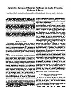
It is proposed to use a sequential estimation approach to solve the extended ML problem. In this approach, the estimation time interval is divided into successive overlapping time slots, referred 7
to as the estimation windows. The ML estimation problem is solved at each estimation window to estimate the unknown parameters. The parameter estimates are then transferred to the next estimation window and used as initial estimates. The unknown parameters consist of some FE model parameters, the values of the base accelerations at each time step over the estimation window, and the simulation error variances. The estimated FE model parameters and simulation error variances are directly transferred from one estimation window to the next and used as initial estimates. The estimated base acceleration time history over the estimation window is subdivided in two parts; the first part, which does not overlap with the next estimation window, is taken as final estimate. The second part, however, is transferred to the next estimation window and used as initial estimate for the next estimation sequence. Figure 1 illustrates schematically the proposed sequential estimation approach. The estimation windows have a constant length (tl = window length in number of time steps) and constant length overlap with the next window (to = length of overlap between two consecutive windows in number of time steps). The sliding (or moving) rate is defined as the difference (in number of time steps) between the starting point of two consecutive windows, i.e., t s t l t o . As shown in Figure 1, the mth estimation window spans from time step t1m to time step t 2m , where t1m t1m1 t s , and t 2m t1m t l . The first part of the estimated base acceleration time history at the mth estimation window, which does not overlap with the next estimation window, is denoted by ˆ gm,m m denotes the second part of the estimated base acceleration time uˆ tgm,:mt m t 1 . Likewise, u t t :t 1
1
s
1
s 2
history that is transferred to the next window as initial estimate.
8
Figure 1: Schematic representation of the proposed sequential estimation approach.
The proposed sequential ML estimation method for the mth estimation window can be summarized as
θˆ , uˆ
g ,m t1m : t2m
, rˆ arg min J y t m : t m , θ, uˆ 1:gt m 1 , utgm,:mt m , r g θ ,u m m ,r t1 : t2
1
2
1
ny ny t2m k 1 g g ,m ˆ J y t m : t m , θ, u1: t m 1 , ut m : t m , r ln rj 1 2 1 1 2 2 j 1 i t1m 2 j 1
1
2
(17)
yij hij θ, uˆ 1:gt m 1 , u tgm,:mi 1
1
rj
2
(18)
in which uˆ 1:g t m 1 is the base acceleration time history from time step 1 to time step t1m 1 , which 1
was estimated in previous estimation windows and is used as a fixed known vector during the mth estimation sequence. The estimation uncertainty is quantified using the parameter estimation covariance matrix, which is approximated asymptotically using the Cramér–Rao lower bound (CRLB). The CRLB is defined as the inverse of the Fisher information matrix (FIM) [31]. Similar to the process shown in [8], the FIM for the sequential estimation problem defined in Eqs. (17)-(18) can be derived as (see Appendix I)
I θθ nθ nθ I θ, utgm,:mt m , r I u g θ 1 2 tl nug nθ 0 ny nθ
where t l nu g
I I θu g
ugug
nθ tl n
tl n
ug
ug
0 n t n y
l
θ
t n l
ug
0 tl nug ny Ir r ny ny
0 n n
ug
y
(19)
is the size of utgm,:mt m , which is the vector of the base acceleration time history to 1
2
th
be estimated at the m estimation window. The sub-matrices I θθ , I θu g , and I u g u g are derived as
I θθ
g ,m ˆg 1 hij θ, u1:t1m 1 , u t1m : i θ j 1 i t1m rj
I θu g
g ,m ˆg 1 hij θ, u1: t1m 1 , ut1m : i θ j 1 i t1m rj
ny
ny
t2m
T
t2m
h θ, uˆ g m , u gm,m 1:t1 1 t1 : i ij θ
g ,m ˆg 1 hij θ, u1: t1m 1 , ut1m : i u tgm,:mt m j 1 i t1m rj 1 2 ny
Iugug
t2m
T
T
h θ, uˆ g m , u gm,m 1: t1 1 t1 : i ij g , m ut m : t m 1 2
h θ, uˆ g m , u gm,m 1: t1 1 t1 : i ij g , m ut m : t m 1 2
(20)
(21)
(22)
9
T Furthermore, it can be shown that I u g θ I θu g . Considering that the FIM given in Eq. (19) is a
block matrix, the lower bound for the covariance matrix of the FE model parameters and the base acceleration time history is simply obtained as Θ I θθ Cov g ,m Ut m : t m I u g θ 1 2
I θu g I u g u g
1
at θ , u gm m , r t1 : t2
(23)
true
where T E Θ E Θ Θ E Θ Θ Cov g ,m Ut m : t m 1 2 E U gm m E U gm m Θ E Θ T t :t t1 :t2 1 2
in
which
E Χ EY
g ,m m | Θ,U m
t1m: t2
m ,R
t1 : t2
U
E Utgm :t m E Utgm :t m 1 2 1 2
θ, u
Χ x p y t
E Θ E Θ
m m 1 :t 2
g ,m t1m :t2m
,r
true
T g E Ut m :t m 1 2
g t1m :t2m
E U tgm :t m 1 2
U
g t1m :t2m
dy t1m :t2m
T
and
(24)
the
matrix
inequality A B means that A B is a positive semidefinite matrix. The right hand side of Eq. (19) is evaluated at the true values (or true state of nature) of the unknown parameters. However, since in a real-world application, the true parameter values are unknown, they are approximated with the corresponding parameter estimates. Considering the asymptotic efficiency of the ML estimation method and assuming the identifiability of the estimation problem ( [32], [33]), θˆ , uˆ tgm,:mt m , and rˆ converge asymptotically to their true values, respectively, when no modeling 1
2
uncertainties exist (i.e., ideal condition). Therefore, the parameter estimation covariance matrix asymptotically converges to the CRLB evaluated at the parameter estimates. Lower bounds for the marginal covariance matrices of the FE model parameters and base acceleration time history can be derived as follows ( [34], [35]).
CovΘ I θθ I θu g I u gu g
1
I u gθ
1
1 g ,m I Cov U I u gθ I θθ I θu g g u g t1m :t 2m u
(25)
1
(26)
Table 1 summarizes the proposed sequential ML estimation algorithm. Table 1: Sequential ML estimation algorithm for output-only nonlinear FE model updating. 1. Set the estimation window length t l , and the sliding rate t s . Find the overlap length t o t l t s . Set t10 t s 1 . 2. Set the initial values: θˆ 0 , rˆ0 . Set uˆ tg0,0:t 0 0 . 1
2
3. For the m estimation window (m = 1, 2, …, N, where N is the number of estimation windows): th
3.1. Set t1m t1m1 t s , and t 2m t1m t l . 3.2. Retrieve the estimated FE model parameters, simulation error variances, and base acceleration
10
time history from the last estimation window (i.e., θˆ m 1 , rˆm 1 , and uˆ tgm,m1:t1m1 ). 1
2
3.3. Set θˆ m , 0 θˆ m1 , and rˆm , 0 rˆm 1 .
ˆ gm,m 3.4. Set uˆ tgm,:mt m t uˆ tgm,m1 1t : t m1 , and u t t 1
1
o
1
s
2
1
m o 1: t2
0 (see Figure 1).
3.5. Solve the optimization problem defined in Eqs. (17)-(18) to find θˆ m , uˆ tgm,:mt m , and rˆm . 1
2
3.6. Find I θθ , I θu g , and I u gu g using Eqs. (20)-(22). 3.7. Compute the CRLB for the estimation covariance matrix of the FE model parameters and the base acceleration time histories using Eqs. (25) and (26), respectively. 3.8. Move on to the next estimation window (m = m + 1) and repeat step 3.
The proposed sequential ML estimation method has two shortcomings that may adversely affect its estimation accuracy and/or computational efficiency: (i)
The ML estimation is asymptotically efficient [31]. This means that, for a large number of informative data samples (e.g., y t m : t m with a large estimation window length t l t 2m t1m ), 1
2
the ML estimator is unbiased and the parameter estimation covariance matrix converges to the CRLB. Thus, to have an efficient estimation, the estimation windows should be long enough. Nevertheless, by increasing the length of the estimation window, the number of estimation parameters and, therefore, the dimension of the optimization problem increase, which in turn requires multiple iterations to find the optimized solution. (ii)
Although the optimal parameter estimates are transferred from one estimation window to the next, no information about their plausibility or degree of belief is transferred between two consecutive windows. The prior probability distribution of the estimation parameters at each estimation window is always assumed to be uniform (non-informative), regardless of the estimation accuracy achieved at the last estimation window. Starting from a noninformative prior at each estimation window results in more iteration to find the optimized solution, which, in turn, increases the computational cost. This important shortcoming is resolved through a sequential maximum a posteriori (MAP) estimation method.
2.2. Sequential MAP estimation method To improve the shortcomings of the sequential ML estimation method, an alternative method is proposed in this section, referred to as the sequential maximum a posteriori (MAP) estimation method. In this method, the posterior joint PDF of the FE model parameters and base acceleration discrete time history is maximized at each estimation window using an iterative linearization approach. Both the posterior mean estimates and covariance matrix of the estimation parameters (which include the input time history) are then transferred to the next estimation window and used as prior information to solve the MAP estimation problem at that window. Therefore, the uncertainties in the estimated model parameters and base acceleration time history is transferred from one estimation window to the next. As will be shown later, this method reduces to an iterative extended Kalman filtering (EKF) approach at each estimation window [36]. 11
Following up on the sequential estimation approach presented in the previous section, the natural logarithm of the posterior joint PDF of the FE model parameters and base acceleration discrete time history at the mth estimation window is derived as
log p θ, utgm,:mt m y t m : t m 1
2
1
2
c log p y
t1m : t2m
θ, utgm,:mt m 1
2
log p θ, u g ,m t1m : t2m
(27)
in which c log p y t m : t m is a normalization constant. In this equation, the time history of 1 2 the base acceleration from time step 1 to t1m 1 , i.e., u1:g t m 1 , is assumed to be deterministic (i.e., 1
known) and equal to the mean estimates obtained from the previous estimation sequences. For notational convenience, an extended parameter vector at the mth estimation window is defined as n t n 1 θ l g
T
u . By substituting Eq. (10) for the likelihood ψ m θT , utgm,:mt m T , where ψ m 1 2 function into Eq. (27) and assuming a Gaussian distribution for the prior joint PDF, it follows that
log p ψ m y t m :t m 1
2
k 12 y 0
t1m : t2m
ht m : t m ψ m , uˆ 1:gt m 1 1
2
1
ψ
T 1 ˆ m Pˆ ψ ψm ψ 2
1
m
T
ˆ ψ
R 1 y t m : t m ht m : t m ψ m , uˆ 1:g t m 1
m
1
2
1
2
1
(28)
where k0 is a constant, and ψˆ m and Pˆ ψ are the prior mean vector and covariance matrix of the ~
t n t n
extended parameter vector at the mth estimation window. The matrix R l y l y is a block diagonal matrix, in which the blocks are defined as the simulation error covariance matrix R , i.e., R n n y y 0 R 0
0 R ny ny tl ny tl ny
0
0
R n n y
y
0
(29)
in which t l t 2m t1m is the estimation window length. To find the MAP estimate of ψ m , the
log p ψ m y t
posterior joint PDF in Eq. (28) is maximized, i.e., h t
m m 1 : t2
ψ , uˆ g
m
ψm
1: t1 1 m
m m 1 : t2
ψm
0 . Therefore,
T
R 1 y t
m m 1 : t2
ht
m m 1 : t2
ψ , uˆ Pˆ ψ g
m
1: t1 1 m
ψ
1
m
ψˆ m 0
(30)
12
Eq. (30), which is a nonlinear algebraic vector equation in ψ m , can be solved iteratively using a m m 1 : t2
ht m : t m 1
2
ψ , u at ψˆ g
first-order approximation of ht
1: t1 1 m
m
ψ m , uˆ 1:g t m 1 ht m : t m ψˆ m , uˆ 1:g t m 1 1
1
2
1
m
as
ht m : t m ψ m , uˆ 1:g t m 1 1
2
1
ψ
ψm ψm
The matrix
ψ
h t
m m 1 : t2
m
, u1:g t
m 1
1
ψ m
m
ψˆ m h.o.t.
(31)
ψˆ m
represents the FE response sensitivities with respect to the
ˆm ψm ψ
extended parameter vector, evaluated at the prior mean of the extended parameter vector, ψˆ m . This matrix is denoted by C hereafter for ease of notation. Substituting Eq. (31) into Eq. (30) and neglecting the higher order terms (h.o.t.) results in the following (first-order approximate) equation for the MAP estimate of ψ m :
ˆ m ψ ˆ m CT R 1C Pˆ ψ ψ
1 1
ˆ m , uˆ 1:g t m 1 CT R 1 y t m : t m h t m : t m ψ 1
2
1
2
1
(32)
in which ψˆ m is the updated (or the posterior) mean estimate of ψ m . It can be shown that the term
C R~ C Pˆ C R~ T
1
ψ
1 1
T
1
is equivalent to the Kalman gain matrix [36]. The updated ψˆ m from Eq.
(32) is iteratively used as the new point for the linearization of ht
m m 1 : t2
ψ , u in Eq. (30) to g
m
1: t1 1 m
find an improved estimate of ψ m . This iterative scheme at each estimation window is equivalent to the iterative EKF method for parameter-only estimation [36]. Following the iterative EKF procedure, the prior covariance matrix of the extended parameter vector Pˆ ψ, m is updated to the posterior covariance matrix Pˆ ψ, m after each iteration until convergence is achieved (i.e., until Eq. (30) is solved within a specified tolerance level). It is moreover assumed that both the prior and posterior joint PDFs of the extended parameter vector are Gaussian. The updated estimation covariance matrix can be obtained as ( [36], [37])
ˆ m Pˆ ψ, m E Ψ m ψ
Ψ
m
ˆ m ψ
T
I KC Pˆ ψ,m I KCT KRK T
(33)
where Ψ m is the random vector representing the unknown extended parameter vector, ψ m , and
~ K CT R 1C Pˆ ψ
C R~
1 1
T
1
is the Kalman gain matrix. Furthermore, to improve the convergence of the iterative EKF procedure, a disturbance is added to the posterior covariance matrix at each iteration to provide the prior covariance matrix for the next iteration, i.e., ˆ ˆ P ψ , i 1 Pψ , i Q
(34)
13
where Q is a constant diagonal matrix with small (relative to the diagonal entries of matrix Pˆ ψ , i ) positive diagonal entries. The matrix Q is referred to as process noise covariance matrix in the Kalman filtering approach ( [36], [37]). The subscript i in Eq. (34) denotes the iteration number. The recursive MAP estimation procedure can be summarized as follows. At each estimation window, the prior estimates of the mean and covariance matrix of the extended parameter vector are updated iteratively following an iterative EKF approach, until some convergence criteria are satisfied. The resulting posterior mean vector and covariance matrix of the extended parameter vector are then transferred to the next estimation window where they are used as prior information. The estimated FE model parameters are directly transferred from one estimation window to the next and used as initial estimates. Transferring the estimated base acceleration time history, however, requires more elaboration. As mentioned earlier, the estimated base acceleration time history over the estimation window is divided in two parts. The first part, which does not overlap with the next estimation window, is taken as final estimate at the end of the iterative EKF process. The second part, however, is transferred to the next estimation window and used as initial estimate for the next estimation sequence. The uncertainties associated with the FE model parameters and the second part of the estimated base acceleration time history are transferred to the next estimation window by deriving the conditional posterior covariance matrix given known values for the first part of the estimated base acceleration time history, based on which the prior covariance matrix of the extended parameter vector for the next estimation window is derived. The process is described in detail in the following section, and is summarized in Table 2. Suppose that the final posterior mean estimate of the extended parameter vector at the (m-1)th estimation window is obtained as (see Figure 1)
ˆ m 1 θˆ Tm 1 , uˆ g ,m 1 ψ t :t
m1 1
T
m1 ts 1
1
, uˆ tg ,mt1 : t m1 1
s
T
m1 2
T
(35)
The final posterior estimate of the covariance matrix of the extended parameter vector for the (m1)th estimation window is correspondingly partitioned as
Pˆ θ θ Pˆ u θ Pˆ u θ
Pˆ ψ, m 1
Pˆ θ u Pˆ u
g ,1
Pˆ u
g ,2
Pˆ θ u
g ,1
g ,1
u
g ,1
g ,2
u
g ,1
Pˆ u Pˆ u
g ,2
g ,1
u
g ,2
g ,2
u
g ,2
(36)
in which utgm,m1:t1m1 t 1 and utgm,m1 1t : t m1 are denoted as u g ,1 and u g , 2 for notational convenience. The 1
1
s
1
s
2
prior mean estimate of the extended parameter vector for the mth estimation window is defined as
ˆ m θˆ Tm 1 , uˆ g , m ψ t :t
m 1
m 1 to
T
, uˆ tg , mt m 1
T
1: t 2
m
o
T
(37)
14
where uˆ tgm,m: t m t uˆ tgm,m1 1t : t m1 is transferred from the previous window, and uˆ tgm,mt 1
1
o
1
s
1
2
as a zero vector, i.e., uˆ tgm,mt 1
m o 1: t2
m o 1: t2
is initialized
0 . The conditional posterior covariance matrix of the estimation
parameters that are transferred from the (m-1)th to the mth estimation window can be derived as Pˆ θ ,u
g,2
u
g ,1
Θ θˆ Θ θˆ T E g , 2 mg ,21 g , 2 mg ,21 uˆ g ,1 U uˆ U uˆ Pˆ θ θ Pˆ u θ g ,2
Pˆ θ u Pˆ u
g ,2
g ,2
u
g ,2
Pˆ θ u Pˆ u u g ,2
Pˆ u
g ,1
g ,1
g ,1
u
g ,1
1
Pˆ θ u Pˆ u u
g ,1
g ,2
g ,1
T
(38)
g , 2 denotes the random vector characterizing u g , 2 (or utgm,m1 1t : t m1 ). Finally, the prior in which U 1
s
2
covariance matrix of the extended parameter vector for the mth estimation window is defined as
Pˆ g , 2 g ,1 ˆP θ,u u ψ 0
ˆP g ,2 g ,2 u u 0
where Pˆ ug ,2 u g ,2 is the prior covariance matrix of utgm,mt 1
m o 1: t2
(39)
which is selected as a diagonal matrix
with identical diagonal entries, i.e., Pˆ ug , 2u g , 2 p 2 t s t s , where denotes the identity matrix, and p is the prior standard deviation of the random (unknown) base accelerations sampled in the time interval t1m t o 1 : t 2m at the mth estimation window. The parameter p is selected as constant for all the estimation windows. Table 2 summarizes the proposed sequential MAP estimation algorithm for output-only nonlinear FE model updating.
It should be noted that unlike in the sequential ML estimation method presented above, the simulation error variances are not estimated in this method. Accurate estimation of the simulation error variances was required to compute the CRLBs in the sequential ML estimation method; however, the estimation accuracy of the sequential MAP estimation method is relatively insensitive to the assumed (initially estimated) values of the simulation error variances. Nevertheless, if needed, the simulation error variances can be treated as unknowns, modeled as random variables, and estimated through the sequential MAP estimation method. For this purpose, the extended parameter vector ψ m can be augmented by including the simulation error variance vector, r , and Eqs. (30) to (33) can be re-derived accordingly. Table 2: Sequential MAP estimation algorithm for output-only nonlinear FE model updating. 1. Set the estimation window length t l , and the sliding rate t s . Find the overlap length t o t l t s . Set t10 t s 1 . 2. Set the initial values: θˆ 0 , Pˆ θθ ,0 , and p . Set uˆ tg ,0:t 0 and Pˆ ug , 2u g , 2 p 2 t s t s . 0 1
0 2
15
3. Set ψ ˆ θˆ T0 0
uˆ tg ,0: t 0 1
T
0 2
T Pˆ , and Pˆ θθ ,0 ψ ,0 0
0 Pˆ u
g ,0
u
g ,0
.
4. Define the process noise covariance matrix Q and the simulation error covariance matrix R . Set up ~ R using Eq. (29). 5. For the mth estimation window (m = 1, 2, …, N, where N is the number of estimation windows): 5.1. Set t1m t1m 1 t s , and t 2m t1m tl . 5.2. Retrieve the posterior estimates of the mean vector and covariance matrix of the extended parameter vector from the last estimation window (i.e., ψˆ , and Pˆ ). ψ , m 1
m 1
ˆ m, 0 ψ ˆ m , where ψˆ m is defined in Eq. (37). 5.3. Set ψ 5.4. Set Pˆ ψ ,m, 0 Pˆ ψ , m , where Pˆ ψ ,m is defined in Eq. (39).
5.5. Iterate (i = 1, 2, …):
ˆ m, i ψˆ m, i 1 , Pˆ ψ , m, i Pˆ ψ , m, i 1 Q . a. Set ψ b. Run the FE model using ψˆ m,i ; obtain FE response and response sensitivities:
yˆ t
m m 1 : t2
ht
m m 1 : t2
ψˆ , uˆ 1:g t m ,i
m 1 1
, C
ht
m m 1 : t2
ψ , uˆ g
m
ψ m
1: t1 1 m
.
ˆ m, i ψm ψ
c. Compute the Kalman gain matrix: K CT R 1C Pˆ ψ, m , i
1 1
CT R 1 .
d. Find the corrected estimates of the mean vector and covariance matrix of the extended parameter vector:
ˆ m, i ψ ˆ m , i K y t m : t m yˆ t m : t m , Pˆ ψ,m, i I KC Pˆ ψ,m, i I KC T KRK T . ψ 1
2
1
2
e. Check for convergence: if ψˆ m , i ψˆ m , i 1 tol1 ψˆ m ,i 1 or i tol2 (where tol1 = tolerance limit for relative change in the estimated parameter vector, and tol2 = max. number of iterations), then move to the next estimation window (m = m + 1, go to step 5); otherwise, iterate again at the current estimation window (i = i + 1, go to step 5.5).
3. Direct differentiation method (DDM) for nonlinear finite element response sensitivity analysis with respect to uniform base excitation DDM is based on the exact (consistent) differentiation of the FE numerical scheme with respect to the sensitivity parameters. As mentioned earlier, the equation of motion, Eq. (1), reduces to a nonlinear algebraic vector equation at each time step when applying a single-step time integration scheme, such as the Newmark-beta method. Following the Newmark-beta method, the acceleration and velocity vectors at time step i are approximated as
16
q i a1 q i a2 q i 1 a3 q i 1 a4 q i 1 , q i b1 q i b2 q i 1 b3 q i 1 b4 q i 1
(40)
where a1 to a4 and b1 to b4 are integration coefficients and can be found in [23]. Substitution of these equations into Eq. (1) results in the following nonlinear vector-valued algebraic equation in q i : a1 M ψ qi ψ b1 C ψ qi ψ γ i q1:i ψ , ψ fi ψ
(41)
~ i 1 ψ fi ψ f i ψ M ψ a 2 q i 1 ψ a 3 q i 1 ψ a 4 q i 1 ψ Cψ b2 q i 1 ψ b3 q i 1 ψ b4 q
(42)
in which
and ψ is the sensitivity parameter vector, i.e., parameters with respect to which the FE response sensitivity is computed. Herein, the sensitivity parameters are the unknown FE model parameters and the values of the base acceleration time history at all time steps. FE response sensitivity computation for FE model parameters using the DDM is well documented in the literature (e.g., [27], [28], [29], [30]). This section describes the FE response sensitivity computation with respect to the discrete time input base acceleration. For the sake of derivation simplicity, it is assumed here that ψ u gj , which is the uniform (or rigid) base acceleration vector at time step j. As mentioned earlier, in the case of earthquake base excitation, the external force vector in Eqs. (41) and (42) takes the form fi M Luig . Eq. (41) gj to obtain the FE response sensitivity with respect to the is differentiated with respect to ψ u uniform base acceleration vector at time step j as
γ i q1:i q i f a1M b1C g ig T q i u j u j
(43)
KTdyn
k
in which the matrix in the left hand side of Eq. (43) is called the dynamic tangent stiffness dyn matrix, K T k 1 and is available from the FE solution if a Newton-Raphson iterative scheme is used to solve Eq. (41) or if at least the consistent (or algorithmic) tangent stiffness matrix γ i q1:i is computed in the last iteration performed to solve Eq. (41) at time step i. The qTi derivation of Eq. (43) recognizes that
γ i q1: i 1 , q, u1:g i u gj
0 . Following Eq. (42), the right q qi
hand side of Eq. (43) is derived as fi u
g j
ML
u ig u
g j
q i 1
u
M a2
g j
a3
q i 1 u
g j
a4
q i 1
q i 1 q i 1 q i 1 C b2 g b3 g b4 g u u j u j u j g j
(44)
17
in which the matrices
q i 1 q i 1 , , and q i 1g are available from the last time step sensitivity gj gj j u u u
computation. Moreover, it is clear that
ig u δ ij n g n g , where δ is the Kronecker delta. u u gj u
Therefore, Eq. (43), which is a linear algebraic equation, can be solved in one-step to compute the FE response sensitivity with respect to the uniform base acceleration vector at time step j, qi . Once Eq. (43) is solved, the sensitivities of the nodal velocity and acceleration response u gj gj can be easily obtained using Eq. (40). The FE response sensitivity vectors with respect to u computation is then repeated at each time step after convergence is achieved for the FE response computation (i.e., solution of Eq. (41)). To provide the required computational tool in this study, the DDM method to compute the nonlinear FE response sensitivities with respect to the uniform base excitation was implemented in the open source finite element analysis software framework OpenSees [38].
4.
Validation study
Numerically simulated structural response data obtained from a three-dimensional (3D) 5-story 2-by-1 bay reinforced concrete (RC) building frame structure subjected to bidirectional horizontal seismic excitation are used to verify the performance of the proposed parameter and input estimation framework. A mechanics-based nonlinear FE model of the building frame, developed in OpenSees [38] is used to simulate the seismic response of the structure. In the simulation phase, the FE model of the structure and the bidirectional seismic input excitation are assumed to be completely known. Simulated structural response quantities are contaminated with artificial measurement noise to represent measured structural response quantities. In the estimation phase, the North-South (NS) component of the base excitation is assumed to be measured and known, while the East-West (EW) component is assumed to be unknown (i.e., unmeasured due to, for example, sensor malfunctioning). Moreover, a set of five FE model parameters characterizing the nonlinear material behavior of the concrete and reinforcing steel are treated as unknown parameters to be estimated. The measured structural dynamic responses are utilized to estimate jointly the five FE model parameters and the full discrete time history of the base acceleration in the EW direction. The two output-only nonlinear FE model updating approaches presented above are implemented in MATLAB [39] and interfaced with OpenSees for FE response and response sensitivity computations. 4.1. 3D RC building frame The building frame has two bays in the EW and one bay in the NS direction, with plan dimensions of 10.0 × 6.0 m (Figure 2). It has a total height of 20.0 m with a uniform story height of 4.0 m. The building is designed as an intermediate moment-resisting RC frame for a moderate seismic risk zone (downtown Seattle, WA) with Site Class D. The resulting design short-period and one-second spectral accelerations are S MS 1.37 g and S M 1 0.53 g , respectively. Dead and live loads and the corresponding seismic masses are calculated according to the 2012 International Building Code [40]. The longitudinal beams have a square cross section of 18
dimensions 0.40 × 0.40 m and are reinforced with 3 #8 longitudinal reinforcement bars at both the top and bottom, and with #3 @ 100 mm as shear reinforcement. The transverse beams have a rectangular cross section of dimensions 0.40 × 0.45 m and are reinforced with 4 #8 longitudinal reinforcement bars at both the top and bottom, and with #3 @ 100 mm as shear reinforcement. The structure has six identical columns with cross-section dimensions 0.45 × 0.45 m reinforced with 8 #8 longitudinal reinforcement bars, and with #3 @ 150 mm as shear reinforcement. Grade 60 reinforcing steel is used for the columns and beams. Figure 2 shows a 3D view of the building frame and the beam and column cross-sections with reinforcement details.
Figure 2: RC building frame: isometric view and beam and column cross-section.
The FE model of the structure is developed using nonlinear fiber-section, displacement-based, beam-column elements, formulated using Bernoulli-Euler beam theory [41]. The material nonlinearity can spread over several integration points along the element, which are called monitored sections. These sections are discretized into fibers, the stress-strain behavior of which is characterized by realistic uniaxial material models (see Figure 3). The concrete material model used is based on the Popovics-Saenz model ( [42], [43]). A typical cyclic stress-strain response of this material model is shown in Figure 4(a). In general, this material model is governed by six parameters, which are subdivided into two primary parameters and four secondary parameters. The two primary parameters ( E c = initial stiffness or Young’s modulus, and f c = concrete compressive strength) are treated as unknown FE model parameters to be identified. The other four parameters are: c = strain at the concrete compressive strength, f cu = concrete ultimate (crushing) strength, u = concrete strain at ultimate strength, and = ratio between the unloading slope from u and the initial stiffness. These parameters are assumed to be known and constant, since the simulated response of the structure is not sensitive to these parameters for the level of earthquake excitation considered in this study. In other words, the concrete material model is not expected to reach its post-peak (softening) branch of response at many concrete 19
fibers, and therefore, these parameters will not be identifiable. As long as their assigned values are physically meaningful, they are not expected to affect the estimation results. The (constant) values of these parameters are selected based on engineering judgement as c 0.004 , f cu 10 MPa , u 0.01 , and 0.2 . The longitudinal steel reinforcing bars are modeled using the modified Giuffré-Menegotto-Pinto material model [44] with smooth curved-shaped loading and unloading branches as illustrated in Figure 4(b). This material model is characterized by eight parameters, which are subdivided into three primary parameters and five secondary parameters. The three primary parameters are: E = elastic (or Young’s) modulus, σ y = initial yield strength, and b = strain-hardening ratio; they are treated as unknown FE model parameters. The five secondary parameters are assumed to be known and constant with the values suggested in [44]. Thus, the FE model parameter vector is T defined as θ E σ y b Ec f c . The true (exact) values of the FE model parameters are 400 MPa , btrue 0.05 , Ectrue 30 GPa , and f c true 40 MPa . taken as E true 200 GPa , σ true y
Figure 3: Hierarchical discretization levels in distributed plasticity structural FE models using fibersection displacement-based beam-column elements (adapted from [7]).
20
(a) (b) Figure 4: Typical cyclic stress-strain behavior of the uni-axial material models used: (a) PopovicsSaenz for the concrete, and (b) Giuffré-Menegotto-Pinto for the reinforcing steel.
The two horizontal ground acceleration records from the 2004 Parkfield earthquake (Cholame 2 west station) are selected for this study [45] (see Figure 5). The nonlinear structural response simulation is performed by first applying the dead loads quasi-statically and then the base excitation dynamically. The nonlinear time history analysis is performed using the Newmark average acceleration method [23] to recursively integrate the equations of motion in time with a constant time step size of t 0.025 sec (equal to the sampling time interval of the ground acceleration record resampled at 40 Hz). The Newton-Raphson method is used to solve iteratively the nonlinear incremental equilibrium equations at each time step. Rayleigh damping [23] is used to model the damping energy dissipation characteristics of the structure, beyond material hysteretic energy dissipation, by assuming a damping ratio of 2% ( [46], [47]) for the first and third modes after applying the gravity loads ( T1 1.43 sec , T2 1.37 sec , and T3 1.30 sec ). It should be noted that the Rayleigh damping coefficients that are used in the estimation phase are identical to those used in the simulation phase. In other words, the Rayleigh damping coefficients are assumed to be known and constant in the estimation phase of this study. The measured structural response time histories consist of the floor absolute acceleration responses at the first, fourth, and fifth (or roof) levels and the relative (to base) roof displacement response. All the responses are measured in both the NS and EW directions at the northeast corner of each level. The acceleration response time histories are polluted with statistically independent, zero-mean, 1% g root-mean-square (RMS) Gaussian white noise processes, while the displacement response time history is polluted with a zero-mean, 5 mm RMS, Gaussian white noise. The noise levels considered are unrealistically high and are unlikely to be seen in the real world; nevertheless, they are considered here to exercise the estimation framework under extreme noisy conditions. Only the strong motion part of the base acceleration time history, which is approximately the first 5 seconds (see Figure 5), is used in this validation study. Nevertheless, the estimation frameworks presented above have been tested successfully for estimating longer input ground motion time histories.
Figure 5: 2004 Parkfield earthquake ground motion (Cholame 2 west station, resampled at 40 Hz); top: 90° component applied in the NS direction; bottom: 360° component applied in the EW direction. 21
4.2. Sequential ML estimation method Two cases as listed in Table 3 are considered to examine the performance of the sequential ML estimation method for output-only nonlinear FE model updating. The two cases differ in the characteristics of the estimation window. The estimation window for Case #1 (EW1) has a length of 100 time steps (i.e., t l 100 0.025 2.5 sec ) and a sliding rate of 50 time steps ( t s 50 0.025 1.25 sec ). By using EW1, the length of the seismic input time history to be estimated (i.e., [0,5] sec) is divided into three estimation windows. The estimation window for Case #2 (EW2) extends over the whole 5 seconds of the seismic input time history to be estimated. In other words, Case #2 is a batch estimation case, in which the entire time history of the base acceleration is estimated jointly with the FE model parameters, and the simulation error variances in a single estimation sequence. Other estimation cases have been investigated and can be found in [48]. Table 3: Validation case studies for the sequential ML estimation method. Case #
Estimation window
Window length
Overlap length
1 2
EW1 EW2
100 200
50 -
Initial estimate of the FE model parameters and base acceleration time history: The initial estimates of the FE model parameters ( θˆ 0 ) are arbitrarily selected as θˆ0,1 0.80 E true , θˆ0,2 1.40 σ true , θˆ0,3 1.20 b true , θˆ0,4 0.80 Ectrue , and θˆ0,4 0.70 f ctrue . The initial estimates of the y
base accelerations are selected as zero as specified in Table 1. The feasible search domains for the FE model parameters and the base acceleration at each time step are selected as 0.5 θˆ 0 θ 2.0 θˆ 0 and 1.0 g uig 1.0 g , respectively. The range of variation of the material
parameter values to be identified is usually relatively narrow and can be estimated using engineering judgement or prior test results on material samples. Nevertheless, a wide range of variation is considered here to examine the accuracy of the estimation method when searching through a large domain. Initial estimate of the simulation error variances: In this study, the simulation error variance corresponds to the measurement noise variance. In a real world application, the statistics of the measurement noise are unknown, but can be approximated by quantifying different sources of measurement noise (e.g., sensor noise, electrical noise, data acquisition system noise, etc.) and adding them appropriately. Here, the true value of the measurement noise variance for the absolute acceleration and relative displacement time histories, which are respectively polluted true 9.6 103 m 2 / s 4 and with 1% g and 5 mm RMS Gaussian white noises, are rAcc true rDisp 2.5 10 5 m 2 . The initial estimate of the simulation error variance is selected as rˆAcc,0 2.17 102 m2 / s4 for the acceleration response data and rˆDisp ,0 9 106 m2 for the displacement response data, which corresponds to 1.5% g RMS and 3 mm RMS measurement 22
noise, respectively. The feasible search domain for the simulation error variance vector is set as 0.1 rˆ0 r 10 rˆ0 . A large search domain was selected for the simulation error variances since in practice, little prior information is available about the amplitude of the measurement noise. Optimization algorithm and convergence criteria: The nonlinear optimization problem defined in Eqs. (17) and (18) is solved using an interior-point method ( [49], [50]) in this study, which is available as a part of the MATLAB optimization toolbox [51]. The convergence criterion for the optimization algorithm is defined by two conditions. The optimization process is considered converged if any of the following two conditions are satisfied. Condition 1: Condition 2:
ˆ ψ ˆ ψ m m 1 ˆ ˆ r r m m 1 J ψ, r
10 4
(45)
2
10 4
(46)
where ψˆ m is the normalized estimated parameter vector at the mth optimization iteration, in which each component of the estimated parameter vector is normalized by the corresponding initial estimate. ... 2 denotes the second order (or Euclidean) norm, and ... denotes the infinity norm (i.e., maximum absolute value of the vector components). Figure 6 compares the true and estimated EW component of the base acceleration time history for the two cases considered. The estimation error time history, which is defined as the difference between the true and estimated base acceleration time histories, is also shown in Figure 6 for each case. It is observed that the EW base acceleration time history is very well estimated in both cases. The base acceleration at the last few time steps is not estimated correctly due to insufficient pertinent information in the measured response of the structure.
(a)
(b) Figure 6: Left: Comparison of the true and estimated base acceleration time history in the EW direction; Right: estimation error time history; (a): Validation Case #1, and (b): Validation Case #2 for the 23
sequential ML estimation method.
Figure 7 shows the standard deviation (S.D.) of the estimated base acceleration time history. It is obtained from the marginal posterior covariance matrix defined in Eq. (26). The S.D.s of the discrete time values of the estimated base acceleration are larger in Case #1 than in Case #2. This means that by increasing the estimation window length, the uncertainties associated with the estimated base acceleration time history decrease.
(a) (b) Figure 7: Standard deviation (S.D.) of the estimated base acceleration time history in the EW direction; (a): Validation Case #1, and (b): Validation Case #2 for the sequential ML estimation method.
Table 4 compares the final estimates of the five unknown FE model parameters normalized by their corresponding true values and the estimated standard deviation of each model parameter (approximated using the CRLB) normalized by the corresponding estimated value, σˆ θi θˆi , which is an estimate of the coefficient of variation (C.O.V.) of the estimated material parameter. This table also reports the relative root mean square error (RRMSE) of the estimated base acceleration time history in the EW direction. The RRMSE is defined as
uˆ k
ˆ1g:k % RRMSE u
i 1
g i
u ig ,true
u ig ,true k
2
100
(47)
2
i 1
Table 4: Comparison of FE model parameter estimation results in Validation Case #1 and Case #2 for the sequential ML estimation method. Final estimates of material parameters Case #
Eˆ
σˆ y
bˆ
Eˆ c
fˆc
f ctrue
Final estimates of C.O.V. (%)
σtrue y
1
1.00
0.99
1.02
1.00
1.00
0.37
0.32
2
1.00
1.00
1.02
1.00
1.01
0.44
0.35
btrue
Ectrue
C.O.V.( Eˆ c )
C.O.V.( fˆc)
(%)
1.78
0.93
1.28
5.24
1.46
1.26
1.48
4.81
C.O.V.( Eˆ ) C.O.V.(ˆ y ) C.O.V.(bˆ)
E true
ˆ g ) RRMSE(u
It is observed that the FE model parameters are estimated with comparable accuracy (i.e., comparable final estimates and C.O.V.) in both cases. Moreover, the RRMSE of the estimated base acceleration time history is small and comparable in both cases. Based on the results 24
presented in Table 4 and Figure 7, it can be concluded that by increasing the estimation window length in Case #2, the accuracy of the estimated base acceleration time history is improved and the associated estimation uncertainty is reduced. The results presented in Table 4 and Figure 6 verify that the estimation algorithm was successful in steering the initial incorrect FE model parameter values to their true values, and simultaneously estimating the base acceleration time history with very good accuracy. Table 5 reports the estimated simulation error variances for the eight measurement channels, normalized by the corresponding true measurement noise variance. The simulation error variance estimation is inaccurate in both Case #1 and Case #2. As shown in Appendix I, the CRLB for the ith component of the simulation error variance vector is asymptotically approximated by 2 k rˆi2 , where k is the total number of data samples used in the estimation process (i.e., k = 100 for Case #1 and k = 200 for Case #2). Therefore, the estimation accuracy of the simulation error variance depends on the number of time samples of the measured data used in the estimation. It should be recognized that incorrect estimation of the simulation error variances adversely affects the estimation of the CRLB for the estimated FE model parameters and base acceleration time history, since the Fisher information matrix defined in Eqs. (20)-(22) depends on the estimated simulation error variances. However, as mentioned earlier, increasing the length of the estimation window, and therefore the number of data samples, increases the computational cost. Table 5: Comparison of the estimated simulation error variances in Validation Case #1 and Case #2 for the sequential ML estimation method. Final estimates of simulation error variance, r / r true Case #
Acc1EW
Acc1NS
Acc4EW
Acc4NS
Acc5EW
Acc5NS
Disp5EW
Disp5NS
1
2.08
1.17
0.63
0.90
0.63
0.96
0.80
0.79
2
0.52
0.88
0.67
1.01
0.63
1.13
0.71
0.78
Figure 8 shows the convergence history of the five FE model parameters for Case #1 and Case #2. The vertical dashed lines in the sub-figures of Figure 8(a) indicate that the iterations have converged for the corresponding estimation window. In this figure, the number of iterations is equal to the number of evaluations of the ML objective function, which in turn is equal to the number of partial FE model runs (from time zero to the time corresponding to the end of the current estimation window). Spike-like behavior is observed in the convergence histories in this figure, which is the result of perturbation in the estimation parameters by the optimization algorithm [51]. Table 6 reports the total number of estimation iterations (which is equal to the total number of FE model runs) and the total wall-clock computation time (in hours) required for Case #1 and Case #2. Each case study was run in parallel on a Dell Precision T7610 desktop workstation using a single Intel Xeon E5-2630 (2.6 GHz) processor with six cores. It is observed that the sequential ML estimation method requires a huge number of iterations and becomes computationally prohibitive for large-scale nonlinear FE models.
25
(a) (b) Figure 8: Convergence history of the estimated FE model parameters; (a): Validation Case #1, and (b): Validation Case #2 for the sequential ML estimation method. Table 6: Comparison of computational (wall-clock) time required by Validation Case #1 and Validation Case #2 for the sequential ML estimation method. Case # 1 2
Total number of iterations
Total computation time (hr)
1227
95
808
168
4.3. Sequential MAP estimation method Two cases, as listed in Table 7, are considered in this section to investigate the performance of the proposed sequential MAP estimation method. The two cases examine the effects of the characteristics of the estimation window on the performance of the proposed estimation method. 26
Other cases have been studied to investigate the effects of convergence criterion and also measurement data type on the performance of the proposed estimation method. These studies are reported in [48]. In both cases, the estimation window has a length of 50 time steps (i.e., tl 50 0.025 1.25 sec ). The sliding rate of the estimation window for Case # 1 (EW1) is 25 time steps (i.e., t s 25 0.025 0.625 sec ), while it is 15 time steps (i.e., t s 15 0.025 0.375 sec ) for the estimation window of Case # 2 (EW2). When using EW1, the estimation interval (i.e., the first five seconds of the earthquake record) is subdivided into seven estimation windows, while it is subdivided into eleven estimation windows when using EW2. EW2 has a wider overlap length than EW1; therefore, the estimation results obtained using EW2 are expected to be more accurate than those obtained using EW1. However, the increase in estimation accuracy when using EW2 is expected to be associated with a higher computational cost than when using EW1. The tolerance parameters for the convergence criterion (see Table 2, step 5.5.e) are set to and for both cases. Table 7: Validation cases studies for the sequential MAP estimation method. Case #
Estimation window
Window length
Overlap length
1 2
EW1 EW2
50 50
25 35
Initial estimate of mean vector and covariance matrix of FE model parameters: The initial estimates of the FE model parameters ( θˆ 0 ) are the same as in the previous validation study using the sequential ML estimation method. The covariance matrix of the initial estimates of the FE model parameter vector, which quantifies the uncertainty in these initial estimates, is selected as a diagonal matrix Pˆ θθ, 0 pθ, i . The term pθ , i , which is the ith diagonal entry of Pˆ θθ, 0 , is the
variance of the initial estimate of the ith FE model parameter and is selected as pθ , i 0.10 θˆ0, i
2
.
Initial estimate of mean vector and covariance matrix of base accelerations: The initial estimates of the base accelerations in the first estimation window are selected as zero (see Table 2, step 2). The covariance matrix of the initial estimates of the base acceleration vector in the first estimation window is selected as a diagonal matrix with identical diagonal entries, i.e., Pˆ ug , 0u g , 0 p 2 t l t l , in which p = 0.05 g and represents the standard deviation of the initial estimate of the base acceleration at each discrete time. Process noise covariance matrix: The process noise covariance matrix Q introduced in Eq. (34), serves the purpose to increase the prior estimation uncertainties and, therefore, increase the relative importance attributed by the estimation algorithm to the measurement data versus the prior information transferred from the last estimation iteration. In other words, the diagonal entries of matrix Q serves as a random disturbance to fuel the search of the estimation algorithm for optimum parameter estimates. A large process noise variance will result in large estimation variability and may result in estimation algorithm instability, but can improve the estimation convergence; a low variance will slow down the convergence of the parameter estimates to their 27
optimum values and may result in non-optimal solutions, but the estimation variability will be low. The matrix Q is selected as a time-invariant (constant) diagonal matrix. The first n θ diagonal entries, which correspond to the FE model parameters, are selected as 10 8 , and the remaining diagonal entries, which correspond to the base accelerations, are selected as 10 4 . Simulation error covariance matrix: In this study, the diagonal entries of the simulation error covariance matrix R (see Eq. (5)), represent the measurement noise variances. As in the previous validation study, the amplitude of the measurement noise is estimated as 1.5% g RMS for acceleration response time histories and 3 mm RMS for displacement response time histories. It should be noted that the process and simulation error covariance matrices have an important effect on the performance and convergence of the estimation process. Further systematic studies to investigate the effects of the process and simulation error covariance matrices on the stability and convergence properties of the sequential MAP estimation method are needed, but out of the scope of this paper. Figure 9 compares the true and estimated EW component of the base acceleration time history for the two validation cases considered here. The estimation error time histories are also shown in Figure 9. It is observed that the EW base acceleration time history is very well estimated in both cases.
(a)
(b) Figure 9: Left: Comparison of the true and estimated base acceleration time history in the EW direction; Right: estimation error time history; (a): Validation Case #1, and (b): Validation Case #2 for the sequential MAP estimation method.
Figure 10 shows the standard deviation (S.D.) of the estimated base acceleration time history. It is obtained from the marginal posterior covariance matrix of the first part of the estimated 28
acceleration time history at each estimation window (i.e., uˆ g ,1 ), which is equal to the submatrix ˆ g ,1 g ,1 in Eq. (36). Figure 10 shows notch points in the estimated S.D. time histories. These P u u notch points are located at the starting point of each estimation window (i.e., t1m , where m denotes the mth estimation window). The structural response data measured across the mth estimation window are most sensitive to uˆ gm and, therefore, there is more information about uˆ gm t1
t1
in the measured response than about other unknown base accelerations over the mth estimation window. Consequently, uˆ gm has a relatively smaller estimation uncertainty than other estimated t1
base accelerations over the mth estimation window. Comparing Figure 10(a) with Figure 10(b) shows that the use of EW2, which has a larger overlap ratio than EW1, results in less uncertainty in the estimated base acceleration time history. In both cases, the estimated S.D. of the estimated base acceleration time history has a right tail, corresponding to the last estimation window, with relatively large estimated S.D. values. The measured response data across the last estimation window have limited information about the base acceleration time history in this window and, therefore, the estimated base accelerations in the last window have relatively larger uncertainties than in the prior estimation windows. Comparing Figures 9 and 10 with Figures 6 and 7, respectively, shows that although the amplitudes of the estimation error time histories are comparable between the two estimation methods, the uncertainties in the base acceleration time histories estimated using the sequential MAP method are overall significantly smaller than those estimated using the sequential ML estimation method.
(a) (b) Figure 10: Estimated standard deviation (S.D.) of the estimated base acceleration time history in the EW direction; (a): Validation Case #1, and (b): Validation Case #2 for the sequential MAP estimation method.
Figures 11-12 show the time histories of the posterior mean (normalized by the corresponding true parameter value) and coefficient of variation (C.O.V.) of the FE model parameters for Case #1 and Case #2, respectively. The vertical dashed lines in these figures indicate that the iteration limit has been reached for each estimation window. It is observed that all the material parameters are iteratively updated from their initial to final estimates, which are converged closely to the corresponding true parameter values with reasonable accuracy and small C.O.V. in both cases. A competing effect between the estimated elastic modulus of steel and concrete is clear. While the elastic modulus of steel is slightly over-predicted, the elastic modulus of concrete is underpredicted. Indeed, the estimation accuracy of elastic moduli will be improved by increasing the length and overlap of the estimation windows and using tight convergence criteria. The 29
estimation time histories of the strength- ( y , f c ) and post-yield ( b ) related material parameters start with a flat-like stage (over the first estimation window) followed by a period of rapid changes, when the structural response becomes nonlinear and sensitive to the strength and post-yield related material parameters after the first estimation window.
Figure 11: Time histories of the posterior mean and C.O.V. of the estimated FE model parameters for Validation Case #1 of the sequential MAP estimation method.
30
Figure 12: Time histories of the posterior mean and C.O.V. of the estimated FE model parameters for Validation Case #2 of the sequential MAP estimation method.
Table 8 reports the final estimates of the material parameters (i.e., the posterior mean estimate of the FE model parameters obtained at the last estimation iteration), the final estimates of the C.O.V. of the material parameters, and the RRMSE of the estimated base acceleration time history in the EW direction as defined in Eq. (47). Table 9 reports the total number of estimation iterations (which is equal to the total number of partial FE model runs) and the total wall-clock computation time (in hours) required for the two cases. As in the first validation study, each case study was run in parallel on a Dell Precision T7610 desktop workstation using a single Intel Xeon E5-2630 (2.6 GHz) processor with six cores. The presented results demonstrate the successful performance of the proposed sequential MAP estimation method for output-only nonlinear FE model updating.
31
Table 8: Comparison of FE model parameter estimation results in Validation Case #1 and Case #2 for the sequential MAP estimation method. Final estimates of material parameters Case #
Eˆ
σˆ y E true
σ true y
bˆ
b true
Eˆ c
E ctrue
fˆc
f c true
Final estimates of C.O.V. (%) C.O.V. ( Eˆ )
C.O.V. (σˆ y )
C.O.V.(bˆ)
C.O.V.( Eˆ c )
C.O.V.( fˆc )
ˆ g ) RRMSE(u
(%)
1
1.02
1.00
1.02
0.95
0.95
0.04
0.02
0.06
0.09
0.10
6.69
2
1.01
1.00
1.02
0.98
0.97
0.03
0.02
0.06
0.08
0.09
5.10
Table 9: Comparison of computational (wall-clock) time required by Validation Case #1 and Validation Case #2 for the sequential MAP estimation method. Case #
Total number of iterations
Total computation time (hr)
1
111
7
2
253
14
4.4. Comparison of the two estimation methods In the sequential ML estimation method, no information about the estimation uncertainty is transferred from one estimation window to the next. This results in a set of only weakly integrated (as compared to the MAP estimation method) optimization problems that are solved sequentially; only the final point estimates (first moment estimates of the parameters) are transferred from one estimation window to the next, where they are used as initial estimates. The efficiency of the estimator depends on the length of the estimation window (i.e., the number of data points across the window). Therefore, an unbiased estimation requires using a relatively long estimation window, which in turn results in increasing the dimension of the optimization problem, and the associated computational cost. In the sequential MAP estimation method, on the other hand, the information obtained about the estimation parameters across an estimation window flows into the next window, by transferring both the parameter estimates and their estimation covariance matrix. The estimation at each window is more strongly integrated (as compared to the ML method) with the previous and next windows, and the efficiency of the estimator depends on the whole time history of the measured response data. The sequential MAP estimation enables using shorter estimation windows than those used in the sequential ML estimation method. Using relatively short estimation windows allows for incremental assimilation of information from the measurement data about the estimation parameters, and improves the overall performance and accuracy of the estimation algorithm. Comparing the estimation results obtained from the two estimation methods shows that the estimation accuracies in all cases presented are similar between the two estimation approaches. This can be concluded by comparing the results presented in Figure 6 vs. Figure 9, Figure 7 vs. Figure 10, and Table 4 vs. Table 8. Nevertheless, the sequential MAP estimation method is computationally much more efficient than the sequential ML estimation method in the presented case studies; this can be concluded by comparing the computational wall-clock times presented in Table 6 and Table 9, respectively. Although the characteristics of the estimation windows are not identical in the case studies presented (due to the reasons mentioned above), there is an order of magnitude difference between the computational wall-clock times of the ML and MAP 32
estimation methods. It should also be noted that the computational efficiency of the two estimation approaches can be optimized by tuning the characteristics of the estimation windows and the convergence criteria. This objective was not pursued in this study. Nevertheless, because of the abovementioned fundamental differences, a significant disparity in the computational demands of the two methods is expected. The computational efficiency of the sequential MAP estimation method makes it a more suitable approach than the sequential ML estimation method for large-scale, nonlinear FE models of civil structures. 5.
Conclusions
This paper presented a novel framework for output-only nonlinear system and damage identification of civil structures. This framework is based on nonlinear finite element (FE) model updating using only the measured structural response to earthquake excitation. A sequential estimation approach was proposed to solve the output-only nonlinear system and damage identification problem. In this approach, the estimation time interval is sub-divided into successive overlapping estimation windows. The estimation problem is solved sequentially over all the estimation windows and at each estimation window, it is solved iteratively to produce a set of estimation results that are transferred to the next estimation window where they are used as prior information. Two method were proposed to estimate sequentially the FE model parameters and the seismic input ground acceleration time histories using only dynamic response measurements: (i) A sequential maximum likelihood (ML) estimation method, which reduces to a sequential nonlinear constrained optimization method. In this method, the unknown FE model parameters, the input ground acceleration time histories, and the simulation error variances (which in this study were equivalent to the measurement noise variances) are estimated jointly using an interior-point method. The estimation uncertainty is quantified using the parameter estimation covariance matrix, which is approximated asymptotically by the Cramér–Rao lower bound (CRLB). Although the estimated parameter values are transferred from one estimation window to the next, no information about the parameter estimation uncertainty is transferred between consecutive estimation windows. The prior probability distribution of the estimation parameters at each estimation window is assumed uniform, regardless of the estimation accuracy achieved at the previous estimation window. Starting from a non-informative prior at each estimation window renders this method computationally expensive and may prelude its use for large-scale, real-world applications. (ii) A sequential maximum a posteriori (MAP) estimation method, which reduces to a sequential iterative extended Kalman filtering method. In this method, the posterior joint PDF of the FE model parameters and base acceleration discrete time histories is maximized at each estimation window using an iterative linearization approach. Estimates of the posterior mean vector and covariance matrix of the estimation parameters are then transferred to the next estimation window where they are used as prior information to solve the MAP estimation problem. Both approaches require the computation of FE response sensitivities with respect to the unknown FE model parameters and the base accelerations at discrete times. The FE response sensitivities were computed accurately and efficiently using the direct differentiation method (DDM). The DDM to compute the FE response sensitivities with respect to a uniform (or rigid) 33
base acceleration discrete time history was implemented in the open source finite element analysis software framework OpenSees. Numerically simulated structural response data from a three-dimensional 5-story 2-by-1 bay reinforced concrete (RC) frame building subjected to bidirectional horizontal seismic excitation were used to verify the performance of the two proposed approaches. While the sequential ML estimation method estimated the unknown FE model parameters and the input ground acceleration time history with acceptable accuracy, it was found to be computationally very expensive. The sequential MAP estimation approach, on the other hand, was found drastically more efficient computationally for a comparable level of estimation accuracy. It thus provides a promising approach for large-scale, real-world applications involving large and complex nonlinear FE models of civil structures. It should be noted that contrary to the sequential ML estimation method, the sequential MAP estimation method is currently an unconstrained estimation process. The model parameters are not constrained to remain in a feasible domain and therefore, they may take unphysical values during the estimation process. This is especially likely when the model parameters are weakly identifiable or unidentifiable. Estimating unphysical values for the model parameters may result in divergence of the FE analysis procedure and consequently, divergence of the estimation process. Efforts are underway to develop a constrained sequential MAP estimation method. The proposed framework can conceptually be applied to different types of structural systems (e.g., buildings, bridges) with different types of structural materials (e.g., reinforced concrete, steel, masonry) to jointly estimate various model parameters (e.g., material, damping, inertia) and different types of input excitation time histories (e.g., base acceleration, forces). Further studies are required to investigate the identifiability of the joint structural system parameter and input identification problem, and develop methods for optimal sensor placement in order to determine the type and number of measurement data channels needed to successfully solve the output-only estimation problem. Acknowledgment The authors wish to thank Dr. Quan Gu at Xiamen University, China, and Dr. Frank McKenna at the Pacific Earthquake Engineering Research (PEER) Center at UC Berkeley for their help with the implementation in OpenSees of the DDM for earthquake ground acceleration input as sensitivity parameters. Their assistance was most valuable and is highly appreciated. Rodrigo Astroza acknowledges the financial support from the Universidad de los Andes – Chile through the research grant Fondo de Ayuda a la Investigación (FAI) and from the Chilean National Commission for Scientific and Technological Research (CONICYT), FONDECYT-Iniciación research project No. 11160009 References [1] S. W. Doebling, C. R. Farrar, M. B. Prime and D. W. Shevitz, "Damage Identification and
Health Monitoring of Structural and Mechanical Systems from Changes in their Vibration Characteristics: A Literature Review," Report LA-13070-MS, Los Alamos, New Mexico, 1996. 34
[2] E. P. Carden and P. Fanning, "Vibration Based Condition Monitoring: A Review,"
Structural Health Monitoring, vol. 3, no. 4, pp. 355-377, 2004. [3] R. Astroza, H. Ebrahimian, J. P. Conte, J. I. Restrepo and T. C. Hutchinson, "System Identification of a Full-scale Five-story Reinforced Concrete Building Tested on the NEESUCSD Shake Table," Structural Control and Health Monitoring, vol. 23, no. 3, pp. 535-559, 2016. [4] E. Ntotsios, C. Karakostas, V. Lekidis, P. Panetsos, I. Nikolaou, C. Papadimitriou and T. Salonikos, "Structural Identification of Egnatia Odos Bridges based on Ambient and Earthquake Induced Vibrations," Bulletin of Earthquake Engineering, vol. 7, pp. 485-501, 2009. [5] B. Moaveni, X. He, J. P. Conte, J. I. Restrepo and M. Panagiotou, "Damage Identification Study of a Seven-Story Full-Scale Building Slice Tested on the UCSD-NEES Shake Table," ASCE Journal of Structural Engineering, vol. 137, no. 6, pp. 705-717, 2011. [6] G. Kerschen, K. Worden, A. F. Vakakis and J. Golinval, "Past, Present and Future of Nonlinear System Identification in Structural Dynamics," Mechanical Systems and Signal Processing, vol. 20, p. 505-592, 2006. [7] H. Ebrahimian, R. Astroza and J. P. Conte, "Extended Kalman Filter for Material Parameter Estimation in Nonlinear Structural Finite Element Models using Direct Differentiation Method," Earthquake Engineering and Structural Dynamics, vol. 44, no. 10, pp. 1495-1522, 2015. [8] H. Ebrahimian, R. Astroza, J. P. Conte and R. A. de Callafon, "Nonlinear Finite Element Model Updating for Damage Identification of Civil Structures using Batch Bayesian Estimation," Mechanical Systems and Signal Processing, DOI: 10.1016/j.ymssp.2016.02.002, 2016. [9] R. Astroza, H. Ebrahimian and J. P. Conte, "Material Parameter Identification in Distributed Plasticity FE Models of Frame-Type Structures Using Nonlinear Stochastic Filtering," ASCE Journal of Engineering Mechanics, vol. 141, no. 5, pp. 04014149 1-17, 2015. [10] C.-H. Huang, "An Inverse Nonlinear Force Vibration Problem of Estimating the External Forces in a Damped System with Time-dependent System Parameters," Journal of Sound and Vibration, vol. 242, no. 5, pp. 749-756, 2001. [11] C.-H. Huang, "A Non-Linear Inverse Vibration Problem of Estimating the External Forces for a System with Displacement-Dependent Parameters," Journal of Sound and Vibration, vol. 248, no. 5, pp. 789-807, 2001. [12] C.-H. Huang, C.-C. Shih and S. Kim, "An Inverse Vibration Problem in Estimating the Spatial and Temporal-dependent External Forces for Cutting Tools," Applied Mathematical Modelling, vol. 33, no. 6, pp. 2683-2698, 2009. [13] M.-H. Lee and Y.-W. Liu, "Input Load Identification of Nonlinear Tower Structural System using Intelligent Inverse Estimation Algorithm," Procedia Engineering, vol. 79, pp. 540549 , 2014. [14] C.-K. Ma and C.-C. Ho, "An Inverse Method for the Estimation of Input Forces Acting on Non-linear Structural Systems," Journal of Sound and Vibration, vol. 275, no. 3-5, pp. 953971, 2004. [15] C.-K. Ma, J.-M. Chang and D.-C. Lin, "Input Forces Estimation of Beam Structures by an 35
Inverse Method," Journal of Sound and Vibration, vol. 259, no. 2, pp. 387-407, 2003. [16] Z. R. Lu and S. S. Law, "Identification of System Parameters and Input Force from Output Only," Mechanical Systems and Signal Processing, vol. 21, no. 5, pp. 2099-2111, 2007. [17] H. Huang, J. N. Yang and L. Zhou, "Adaptive Quadratic Sum-Squares Error with Unknown Inputs for Damage Identification of Structures," Structural Control and Health Monitoring, vol. 17, no. 4, pp. 404-426, 2010. [18] E. Lourens, C. Papadimitriou, S. Gillijns, E. Reynders, G. De Roeck and G. Lombaert, "Joint Input-Response Estimation for Structural Systems based on Reduced-order Models and Vibration Data from a Limited Number of Sensors," Mechanical Systems and Signal Processing, vol. 29, pp. 310-327, 2012. [19] A. Al-Hussein and A. Haldar, "Novel Unscented Kalman Filter for Health Assessment of Structural Systems with Unknown Input," ASCE Journal of Engineering Mechanics, vol. 141, no. 7, p. 04015012, 2015. [20] S. Eftekhar Azam, E. Chatzi and C. Papadimitriou, "A Dual Kalman Filter Approach for State Estimation via Output-Only Acceleration Measurements," Mechanical Systems and Signal Processing, Vols. 60-61, pp. 866-886, 2015. [21] F. Naets, J. Croes and W. Desmet, "An Online Coupled State/Input/Parameter Estimation Approach for Structural Dynamics," Computer Methods in Applied Mechanics and Engineering, vol. 283, pp. 1167-1188, 2015. [22] F. Naets, J. Croes and W. Desmet, "Stable Force Identification in Structural Dynamics using Kalman Filtering and Dummy-Measurements," Mechanical Systems and Signal Processing, Vols. 50-51, pp. 235-248, 2015. [23] A. K. Chopra, Dynamics of Structures: Theory and Applications to Earthquake Engineering, Englewood Cliffs, N.J.: Prentice-Hall, 4th Ed., 2012. [24] J. L. Beck and L. S. Katafygiotis, "Updating Models and their Uncertainties. Part I: Bayesian Statistical Framework," ASCE Journal of Engineering Mechanics, vol. 124, no. 4, pp. 455-461, 1998. [25] J. L. Beck, "Bayesian System Identification based on Probability Logic," Structural Control and Health Monitoring, vol. 17, no. 7, p. 825–847, 2010. [26] H. Ebrahimian, R. Astroza and J. P. Conte, "Output-only Identification of Civil Structures using Nonlinear Finite Element Model Updating," in SPIE 9438, Health Monitoring of Structural and Biological Systems, San Diego, CA, 2015. [27] C. A. Vidal, H.-S. Lee and R. B. Haber, "The Consistent Tangent Operator for Design Sensitivity Analysis of History-Dependent Response," Computing Systems in Engineering, vol. 2, no. 5-6, pp. 509-523, 1991. [28] M. Kleiber, H. Antunez, T. D. Hien and P. Kowalczyk, Parameter Sensitivity in Nonlinear Mechanics: Theory and Finite Element Computations, New York, N.Y.: John Wiley & Sons, 1997. [29] Y. Zhang and A. Der Kiureghian, "Dynamic Response Sensitivity of Inelastic Structures," Computer Methods in Applied Mechanics and Engineering, vol. 108, no. 1-2, p. 23–36, 1993. [30] J. P. Conte, P. K. Vijalapura and M. Meghella, "Consistent Finite-Element Response Sensitivity Analysis," ASCE Journal of Engineering Mechanics, vol. 129, no. 12, p. 1380– 36
1393, 2003. [31] T. K. Moon and W. C. Stirling, Mathematical Methods and Algorithms for Signal Processing, Upper Saddle River, N.J.: Prentice-Hall, 2000. [32] G. C. Goodwin and R. L. Payne , Dynamic System Identification: Experiment Design and Data Analysis, New York, N.Y.: Academic Press, 1977. [33] S. M. Kay, Fundamentals of Statistical Signal Processing. Volume 1: Estimation Theory, Upper Saddle River, N.J.: Prentice Hall, 1993. [34] P. Tichavsky, C. H. Muravchik and A. Nehorai, "Posterior Cramer–Rao Bounds for Discrete-Time Nonlinear Filtering," IEEE Transactions on Signal Processing, vol. 46, no. 5, pp. 1386-1396, 1998. [35] H. L. Van Trees, Optimum Array Processing, Part IV of Detection, Estimation, and Modulation Theory, New York, N.Y.: John Wiley & Sons, 2002. [36] D. Simon, Optimal State Estimation: Kalman, H Infinity, and Nonlinear Approaches, Hoboken, N.J.: John Wiley & Sons, 2006. [37] R. S. Bucy and P. D. Joseph, Filtering for Stochastic Processes with Applications to Guidance, New York, N.Y.: John Wiley & Sons, 1968. [38] OpenSees, "Open System for Earthquake Engineering Simulation," [Online]. Available: http://opensees.berkeley.edu/. [Accessed 08 2015]. [39] "MATLAB (2012)," The MathWorks Inc., Natick, Massachusetts, United States. [40] International Code Council, 2012 International Building Code, Country Club Hills, 2011. [41] F. F. Taucer, E. Spacone and F. C. Filippou, "A Fiber Beam-Column Element for Seismic Response Analysis of Reinforced Concrete Structures," UBC/EERC 91-17, Earthquake Engineering Research Center, College of Engineering, UC Berkeley, Berkeley, CA, 1991. [42] T. A. Balan, F. C. Filippou and E. P. Popov, "Constitutive Model for 3D Cyclic Analysis of Concrete Structures," ASCE Journal of Engineering Mechanics, vol. 123, no. 2, p. 143–153, 1997. [43] A. Zona, M. Barbato and J. P. Conte, "Finite Element Response Sensitivity Analysis of Continuous Steel-Concrete Composite Girders," Steel and Composite Structures, vol. 6, no. 3, pp. 183-202, 2006. [44] F. C. Filippou, E. P. Popov and V. V. Bertero, "Effects of Bond Deterioration on Hysteretic Behavior of Reinforced Concrete Joints," EERC Report 83-19, Earthquake Engineering Research Center, College of Engineering, UC Berkeley, Berkeley, CA, 1983. [45] "Center for Engineering Strong Motion Data, CESMD - A Cooperative Effort," [Online]. Available: http://strongmotioncenter.org/. [Accessed 08 2015]. [46] M. Panagiotou, Seismic Design, Testing and Analysis of Reinforced Concrete Wall Buildings, Ph.D. Thesis, Department of Structural Engineering, University of California San Diego, La Jolla, CA, 2008. [47] ATC Task Group 7, "Modeling and Acceptance Criteria for Seismic Design and Analysis of Tall Buildings," PEER/ATC 72-1, Pacific Earthquake Engineering Research Center, Richmond, CA, 2010. [48] H. Ebrahimian, Nonlinear Finite Element Model Updating for Nonlinear System and Damage Identification of Civil Structures, Ph.D. Thesis, Department of Structural 37
Engineering, University of California San Diego, La Jolla, CA, 2015. [49] R. H. Byrd, M. E. Hribar and J. Nocedal, "An Interior Point Algorithm for Large-scale Nonlinear Programming," SIAM Journal on Optimization, vol. 9, no. 4, p. 877–900, 1999. [50] R. H. Byrd, J. C. Gilbert and J. Nocedal, "A Trust Region Method Based on Interior Point Techniques for Nonlinear Programming," Mathematical Programming, vol. 89, no. 1, pp. 149-185, 2000. [51] The MathWorks, "MATLAB Optimization Toolbox, User's Guide, R2014a," The MathWorks Inc., Natick, MA, 2014. Appendix I: Derivation of the (Exact) Fisher Information Matrix T The Fisher information matrix (FIM) is defined as I E s s where s ... denotes the score
function and the expectation is taken with respect to the conditional joint PDF
θ, u , r with conditioning on the FE model parameters, base acceleration time
p yt
true
g ,m
m
1
m m t1 : t2
m
: t2
history, and simulation error variances inside the mth estimation window. The score function is defined as the gradient of the log-likelihood function with respect to the parameters to be estimated [31]. For the ML estimation problem stated in Eqs. (17)-(18), the score function can be derived as
s θ, r , uˆ 1:g t
m 1
1
, u tg ,:mt , y t m 1
m 2
m m 1 : t2
m 1
m 1
m 2
m 1
m 2
m 1
m 1
m 2
m 1
m 2
m 1
m 2
m 1
m 2
θ, r , uˆ g , u g , m y 1: t 1 t :t t :t θ θ, r, uˆ 1:g t 1 , u tg ,:mt y t : t u tg ,:mt g ,m ˆg θ, r , u1: t 1 , u t : t y t : t r m 1
T
m 2
m 1
T T
(I1)
in which is the log-likelihood function defined as the natural logarithm of the likelihood function defined in Eq. (10), i.e.,
θ, r , u t
g ,m m m 1 : t2
, yt
m m 1 : t2
n t tl ny t 1 ln 2π l ln rj y i yˆ i θ, u tg ,:mi 2 2 j 1 2 i t
y
m 1
where yˆ i θ, utgm,:mi hi θ, uˆ 1:g t m 1 , utgm,:mi 1
m 2
1
1
m 1
T
R 1 y i yˆ i θ, u tg ,:mi m 1
(I2)
is the FE predicted structural response vector at time step
i and the dependence of yˆ i on uˆ 1:g t m 1 is dropped to ease the notation. Substituting Eq. (I2) 1
into Eq. (I1) yields
38
t yˆ θ, u g , m T t :i i R 1 y yˆ θ, u g , m i i t :i i t θ T t yˆ i θ, u tg ,:mi R 1 y yˆ θ, u g , m i i g ,m t :i u i t t :t t 1 t l r 1 w i 2 2 i t m 2
m 1
m 1
s θ, r , uˆ 1:g t
, ut 1
g ,m
m 1
m m 1 : t2
, yt
m m 1 : t2
m 2
m 1
m 1
m 1
m 1
m 1
m 2
m 2
m 1
in which r
1
1 r1
1 r2
1 ... rny
y yˆ θ, u g , m t :i i1 i1 wi 2 r1 m 1
(I3)
T
2
and the vector w i is defined as
yi 2 yˆ i 2 θ, u tg ,:mi m 1
2
...
2 2
r
yin yˆ in θ, u tg ,:mi y
y
m 1
2 ny
r
2
T
(I4)
It should be noted that the derivative of vector a m1 with respect to vector b n1 is denoted as C
a , where C is a m n matrix defined as cij ai . The FIM, which is b b j
symmetric, can be obtained as
I θ, u tg ,:mt m 1
m 2
I θθ n n , r I u θ t n n I r θ n n
θ
θ
g
l
u
y
θ
g
θ
I I θu
g
u u
g
g
nθ tl n
tl n
I ru
g
u
g
u
g
I θr n n
t n l
ny tl n
u
g
u
u r t n n I rr n n θ
g
I
y
g
l
u
y
(I5)
y
g
y
The submatrix I θθ in Eq. (I5) can be derived as
39
g ,m ˆg θ, r, u1:t1m 1 , u t1m :t2m , Yt1m :t2m I θθ E θ
t2m yˆ i θ, utgm.m:i 1 E m θ i t1
yˆ θ, u gm,m i t1 : i m m θ i t1 j t1 t2m
t2m
yˆ θ, u gm,m i t1 : i m θ i t1 t2m
T
R
1
T
θ, r, uˆ g m , u gm,mm , Y m m 1:t1 1 t1 :t2 t1 :t2 θ
i
g ,m t1m : i
i
j
j
j t1m
R 1 E Yi yˆ i θ, u tgm,:mi 1
T
g ,m t1m : j
Y yˆ θ, u j
T
g ,m t1m : j
j
R δij
T
yˆ θ, u gm,m i t1 : i R 1 θ
yˆ θ, u gm,m j t1 : j R θ
Y yˆ θ, u Y yˆ θ, u t2m
T
1
g ,m 1 yˆ j θ, u t1m : j R θ
(I6)
where the measured structural response in the mth estimation window is modeled as a random m m 1 : t2
E Yi yˆ i θ, utg ,:mi m 1
. Eq. (I6) uses the relation Yi yˆ i θ, utg ,:mi Vi r , which implies that
vector denoted by Yt
assuming that θ, r, u
g ,m t1m : i
m 1
are the true values of these quantities. Therefore, it
can be concluded that
g ,m ˆg 1 hij θ, u1:t1m 1 , u t1m : i I θθ θ j 1 i t1m rj The submatrix I θu g in Eq. (I5) can be obtained as t2m
ny
I θu g
g ,m ˆg θ, r, u1: t1m 1 , ut1m : t2m , Yt1m : t2m E θ
t2m g ,m yˆ i θ, ut1m :i E m θ i t1
yˆ θ, u gm,m i t1 : i θ i t1m j t1m t2m
t2m
yˆ θ, u gm,m i t1 : i m θ i t1 t2m
T
R
1
T
θ, r, uˆ g m , u gm,m m , Y m m 1: t1 1 t1 : t2 t1 : t2 g ut m : t m 1 2
i
g ,m t1m : i
i
j
R 1 E Yi yˆ i θ, utgm,:mi 1
j
j
T
g ,m t1m : j
g ,m t1m : j
(I7)
Y yˆ θ, u
R δij
j
j t2m
Y yˆ θ, u Y yˆ θ, u
yˆ θ, u gm,m i t1 : i R u gm,mm t1 : t2 1
h θ, uˆ g m , u gm,m 1:t1 1 t1 :i ij θ
t2m
T
T
T
T
yˆ θ, u gm,m j t1 : j R u gm,mm t1 : t2 1
g ,m 1 yˆ j θ, ut1m : j R g ,m ut1m : t2m
(I8)
Therefore,
40
g ,m ˆg 1 hij θ, u1: t1m 1 , u t1m : i θ j 1 i t1m rj t2m
ny
I θu g
T
h θ, uˆ g m , u gm,m 1: t1 1 t1 : i ij g , m ut m : t m 1 2
(I9)
The third submatrix in Eq. (I5), I θr , can be derived as
g ,m ˆg θ, r, u1:t1m 1 , ut1m : t2m , Yt1m : t2m I θr E θ tm tl 2 E 2 i t1m
yˆ θ, u gm,m t1 : i i θ
g ,m tm t 2 yˆ i θ, ut1m : i l 2 i t1m θ
T
R
1
T
θ, r, uˆ g m , u gm,mm , Y m m 1:t1 1 t1 : t2 t1 : t2 r
1
r
g ,m t1m : i
r
Yi yˆ i θ, utgm,:mi
1 T
T
R E Yi yˆ i θ, u 1
1 T
0
g ,m tm 1 2 yˆ i θ, ut1m : i 2 i t1m θ
T
t m t m y ˆ i θ, utgm,:mi 1 2 2 1 2 i t1m j t1m θ
R
1
Yi yˆ i θ, utgm,:mi
T
1
m W j t1 t2m
T j
R 1 E Yi yˆ i θ, utgm,:mi 1
W
(I10) T j
in which the vector w i , as defined in Eq. (I4), is modeled as a random variable denoted by Wi . Using Eq. (I4), the term E Yi yˆ i θ, utg ,:mi WjT can be developed as
E Yi yˆ i θ, utgm,:mi 1
m 1
2 E Yi1 yˆi1 Y j1 yˆ j1 r12 2 E Yi 2 yˆi 2 Y j1 yˆ j1 2 WTj r1 E Y yˆ Y yˆ 2 iny j1 j1 iny 2 r1
1
Y
t2 n
1
yˆ t n 2
2
2 E Yi 2 yˆi 2 Y j 2 yˆ j 2 r22
E Yi 2 yˆi 2 Y jny yˆ jny rn2y
E Yiny yˆiny
Y
j2
E Yiny yˆiny
2 yˆ j 2
2 2
Y
jny
2 ny
r
r
E Yi1 yˆi1 Y jny yˆ jny rn2y
The components of this matrix are in the form E Yt1m yˆ t1m Yt 2n yˆ t 2n 2 m n , it is clear that E Yt m yˆt m
2 E Yi1 yˆi1 Y j 2 yˆ j 2 r22
. When
yˆ jny
2 2
2
t1 t 2 or
E Y yˆ E Y yˆ 2 0 tm tm tn tn 1
1
2
2
0
On the other hand, when t1 t 2 and m n , due to the symmetry of the Gaussian probability distribution assumed for the measurement noise, it follows that
E Yt1m yˆ t1m
Yt n yˆt n 2 2
2
E Yt1m yˆ t1m 3 0
Therefore, E Yi yˆ i θ WTj 0 , and from Eq. (I10), it follows that Iθr ITrθ 0 . Similarly, it can be shown that I u g r IT g 0 . ru
41
The submatrix I u g u g in Eq. (I5) can be derived as Iugug
g ,m ˆg θ, r, u1: t1m 1 , ut1m : t2m , Yt1m : t2m E utgm,:mt m 1 2
tm g ,m 2 yˆ i θ, ut1m : i E g ,m m i t1 ut1m : t2m
yˆ θ, u gm,m i t1 : i g ,m m m u i t1 j t1 t1m : t2m t2m
t2m
yˆ θ, u gm,m i t1 : i g ,m ut m : t m i t1m 1 2 t2m
T
T
θ, r, uˆ g m , u gm,mm , Y m m 1: t1 1 t1 : t2 t1 : t2 g ,m u t m : t m 1 2
R 1 Y yˆ θ, u g ,m i i t1m : i
T
Y yˆ θ, u j
j
j t2m
yˆ θ, u gm,m i t1 : i R u gm,mm t1 : t2 1
T
g ,m t1m : j
Y yˆ θ, u j
g ,m t1m : j
j
R δij
T
t2m
R 1 E Yi yˆ i θ, utgm,:mi 1
T
yˆ θ, u gm,m j t1 : j R u gm,mm t1 : t2 1
g ,m 1 yˆ j θ, ut1m : j R u gm,mm t1 : t2
(I11)
Therefore, it follows that Iugug
g ,m ˆg 1 hij θ, u1: t1m 1 , ut1m : i utgm,:mt m j 1 i t1m rj 1 2 ny
t2m
T
Finally, the last submatrix in Eq. (I5), I rr , can be obtained as T ˆ g m , u gm,mm , Y m m θ, r, uˆ g m , u gm,mm , Y m m θ , r , u 1: t1 1 t1 : t2 t1 : t2 1: t1 1 t1 : t2 t1 : t2 I rr E r r
t2m
t2m
2 l
h θ, uˆ g m , u gm,m 1: t1 1 t1 : i ij g , m ut m : t m 1 2
t2m
(I12)
(I13)
t2m
T t 1 1 T tl 1 t 1 r r r E WiT l E Wi r 1 E Wi W Tj 4 4 i t1m 4 i t1m 4 i t1m j t1m From Eq. (I4), it can be found that
E Y yˆ θ, u g , m t :i i1 i1 E Wi r12 1 r1
1 r2
...
m 1
1
2
E Yi 2 yˆ i 2 θ, u tg ,:mi
m 1
r22
2
E Yin yˆ in θ, u tg ,:mi ...
y
y
rn2 y
m 1
2
T
T
1 r rn y
From Eq. (I4), the term E Wi WTj can be developed as
42
E Y yˆ 2 Y yˆ 2 i1 i1 j1 j1 4 r1 2 2 E Yi 2 yˆ i 2 Y j1 yˆ j1 T E Wi W j r22 r12 2 Y j1 yˆ j1 2 E Yiny yˆ iny rn2 r12 y
E Yi1 yˆ i1 2 Y j 2 yˆ j 2 2
r12 r22
E Yi 2 yˆ i 2 2 Y j 2 yˆ j 2 2
r24
E Y
iny
yˆ iny 2 Y j 2 yˆ j 2 2
rn2 r22 y
E Yi1 yˆ i1 2 Y jny yˆ jny 2
E Yi 2 yˆ i 2 2 Y jny yˆ jny 2 r22 rn2 y 2 2 E Yiny yˆ iny Y jny yˆ jny 4 rn y r12 rn2
y
The components of this matrix are in the form E Yt1m yˆ t1m 2 Yt 2n yˆ t 2n 2 . When t1 t 2 or m n , it follows that
E Yt1m yˆ t1m
Y 2
t 2n
yˆ t2n
E Y
E Y
E Yt1m yˆ t1m
2
2
t 2n
yˆ t2n
ˆ 2 Yt 2 n yˆ t 2n 2 However, when t1 t 2 and m n , the term t1m y t1m Gaussian assumption of the zero-mean measurement noise,
E Yt m yˆ t m 1
1
Y 2
t n 2
yˆ t
2
n
2
r 2
r
m n
reduces to, from the
E Y yˆ 4 3 r 2 m t m t m 1
1
From the above, the last term in Eq. (I13) (double sum) can be developed as 1 r2 1 1 t2m t2m m m E Wi WTj tl2 tl r2 r1 i t1 j t1 1 rny r1
1 r1rny 1 r2 rny tl 1 rn2y
1 r1r2 1 r22 1 rny r2
3 r2 1 1 r2 r1 1 rny r1
1 r1r2 3 r22 1 rny r2
1 r1rny 1 r2 rny 3 rn2y
from which
t2m
t2m
E W W i
i t1m j t1m
T j
t r 2 l
1
r
1 T
1 r2 1 0 2tl 0
0 1 r22
0
0 0 1 rn2y
Therefore, from Eq. (I13), submatrix I rr can be expressed as
43
T T T T t2 t2 t2 t2 I rr l r 1 r 1 l r 1 r 1 l r 1 r 1 l r 1 r 1 4 4 4 4
1 r2 1 tl 0 2 0
0 1 r22
0
0 0 1 rn2y
from which 1 r2 1 tl 0 I rr 2 0
0 1 r22
0
0 0 1 rn2y
(I14)
44