I. INTRODUCTION
Bearing Estimation via Spatial Sparsity using Compressive Sensing
ALI CAFER GURBUZ, Member, IEEE TOBB University of Economics and Technology VOLKAN CEVHER, Member, IEEE Ecole Polytechnique Federale de Lausanne JAMES H. McCLELLAN, Fellow, IEEE Georgia Institute of Technology
Bearing estimation algorithms obtain only a small number of direction of arrivals (DOAs) within the entire angle domain, when the sources are spatially sparse. Hence, we propose a method to specifically exploit this spatial sparsity property. The method uses a very small number of measurements in the form of random projections of the sensor data along with one full waveform recording at one of the sensors. A basis pursuit strategy is used to formulate the problem by representing the measurements in an overcomplete dictionary. Sparsity is enforced by `1 -norm minimization which leads to a convex optimization problem that can be efficiently solved with a linear program. This formulation is very effective for decreasing communication loads in multi sensor systems. The algorithm provides increased bearing resolution and is applicable for both narrowband and wideband signals. Sensors positions must be known, but the array shape can be arbitrary. Simulations and field data results are provided to demonstrate the performance and advantages of the proposed method. Manuscript received November 10, 2009; revised September 6, 2010; released for publication May 10, 2011. IEEE Log No. T-AES/48/2/943822. Refereeing of this contribution was handled by T. Luginbuhl. This work was supported by the Marie Curie IRG Grant “Compressive Data Acquisition and Processing Techniques for Sensing Applications” with Grant PIRG04-GA-2008-239506, and an AROMURI Grant: “Multi-Modal Inverse Scattering for Detection and Classification of General Concealed Targets,” Contract DAAD19-02-1-0252. Authors’ addresses: A. C. Gurbuz, Department of Electrical and Electronics Engineering, TOBB University of Economics and Technology, Sogutozu Cad. No. 43, Sogutozu, Anakara, 06560, Turkey, E-mail: (
[email protected]); V. Cevher, Ecole Polytechnique Federale de Lausanne, Laussanne, Switzerland (with joint appointment at the Idiap Research Institute, Martigny, Switzerland); J. H. McClellan, School of Electrical and Computer Engineering, Georgia Institute of Technology, Atlanta, GA 30332-0250. c 2012 IEEE 0018-9251/12/$26.00 ° 1358
Source localization [1, 2] is of great interest in many areas including array signal processing, sensor networks, remote sensing, and wireless communications. Several methods exist to address the problem of estimating the direction of arrivals (DOAs) of multiple sources [3] using the signals received at the sensors. The most commonly used methods include generalized cross correlation (GCC), beamforming, minimum variance distortionless response (MVDR), multiple signal classification (MUSIC) algorithms, and subspace-based methods like Root-MUSIC and ESPRIT, estimation of signal parameters via a rotational invariant technique. These algorithms acquire the source signals at the Nyquist rate and must transmit all measurements to a central processor in order to estimate just a small number of source bearings. The communication load between sensors can be drastically reduced, however, by exploiting spatial sparsity, i.e., the fact that the number of sources we are trying to find is much less than the total number of possible source bearings. The sparsity property of signals has been utilized in a variety of applications including image reconstruction[4], medical imaging [5], radar imaging [6], blind source separation [7], and shape detection [8]. In the literature, sparsity information has also been used previously for beamforming and source localization [9—11]. In [9] the DOA estimation of narrowband sources impinging on a uniform circular array was considered, and `1 regularization was applied with an error constraint applied in angle space to a small number of conventional beamformer outputs. In [10] the `1 norm of the signal energies for narrowband sources was minimized subject to a constraint on the `2 norm of the measurement errors. This formulation leads to second-order cone (SOC) programming where the optimization is performed over the entire signal space. The very high computational complexity of this formulation can be reduced by introducing the singular value decomposition (SVD) of the measured data matrix. The method in [11] tries to reconstruct the signals for sparse sources in the time domain with a combined `1 —`2 norm minimization similar to [10]. In [12] a new hardware architecture exploiting compressive sensing (CS) for direction estimation is also used. Although prior research has validated the benefits of exploiting spatial sparsity in source localization, such as improved resolution, the methods also require a high sampling rate of source signals, which increases the communication load between sensors. This is an important consideration for energy efficient wireless sensor networks. Furthermore, in some applications, data acquisition might be very expensive. For example, the Allen Telescope Array northeast of San Francisco has a frequency
IEEE TRANSACTIONS ON AEROSPACE AND ELECTRONIC SYSTEMS VOL. 48, NO. 2 APRIL 2012
coverage from 0.5 to 11.2 GHz for scientific studies. Moreover, most algorithms assume narrowband source signals. Our goal is to exploit the spatial sparsity of sources to accomplish source localization in arbitrary shaped sensor arrays for both narrowband and wideband signals by using a very small number of measurements, thereby improving the communication efficiency of sensor networks. CS [13—15] is a recently developed mathematical framework, which asserts that a sparsely representable signal can be reconstructed using a small number of linear measurements. For example, consider a signal x = ª s, which is sparse in the basis defined by the columns of ª . According to CS, if nontraditional linear measurements y = ©x in the form of randomized projections are taken, the signal x can be exactly reconstructed with a high probability from M = C(¹2 (©, ª ) log N)K compressive measurements [16] where ¹2 (©, ª ) is the mutual coherence between © and ª , by solving a convex optimization problem of the following form: min ksk1
subject to y = ©ª s
(1)
which can be solved efficiently with linear programming. The key result is that the required number of measurements is linked linearly to the sparsity K of the signal. In our application to source localization, we do not place any sparsity constraints on the source signals; rather, we only assume sparsity in the bearing domain, i.e., spatial sparsity, so that the “signal” we are trying to reconstruct is the bearing domain vector, not the source signals themselves. We cannot, however, take compressive measurements (random projections) of the bearing vector directly. Instead, we are only able take random projections of the received signals at the sensors, which in turn can be linearly modeled as delayed and weighted combinations of multiple source signals at different bearings. These are used in our formulation to find the bearing domain vector; see [17], [18]. Reconstructing the linear relation between the bearing vector and the received signals at the sensors requires construction of a dictionary of source signals. The problem of finding an “optimal” representation in terms of the given dictionary elements can be formulated in terms of basis pursuit [19, 20]. We use this basis pursuit strategy to formulate the source localization problem as a dictionary selection problem where the dictionary entries are produced by synthesizing the sensor signals for each discrete bearing on a grid of possible bearings. Spatial sparseness implies that only a few of the dictionary entries will be needed to match the measurements. When the source signals are known, e.g., as in active radar, it is possible to directly create the dictionary entries by delaying the known reference
signals [6, 21]. When the source signals are unknown but incoherent, we show that we can eliminate the high-rate analog-to-digital converters (ADCs) from all but one of the array elements by using CS to perform the beamforming calculation. We must devote one sensor to acquiring a reference signal, and this operation must be done at a high rate, i.e., Nyquist-rate sampling; the other sensors only need to do compressive sampling. Practical applications of such sensors are shown in [22]. By using the data from the reference sensor, we show that one can relate the compressive measurements at all other sensors to the bearing domain vector linearly, because we assume that although the locations of the sensors can be arbitrary, their locations with respect to the reference sensor are known. This enables us to use sparsity information within a regularization framework; hence the sparse bearing vector can be found by solving an `1 minimization problem, which is detailed in Section II. Our compressive bearing estimation approach based on spatial sparsity has several advantages over other approaches in the literature, such as GCC, MVDR, MUSIC, and previous methods using sparsity [9—11], which require Nyquist sampling at the sensors. Creating a bearing spectrum with many fewer measurements decreases the communication load in wireless networks and enables lower data acquisition rates, which might be very important for high bandwidth applications. Moreover, the array geometry can be arbitrary but known. Other advantages include increased resolution and robustness to noise. The optimization is done over convex functionals; hence, an accurate initialization is not required and the global minimum can be found. Also since the optimization is done over the angle space only, rather than over all signal spaces as in [10], [11], the problem dimensions are much smaller, thereby reducing the computational complexity of our algorithm. While previous methods could locate up to L ¡ 1 sources where L is the number of sensors for uniform arrays, the proposed method can also locate more sources than the number of sensors, without breaking the spatial sparsity assumption. The organization of the paper is as follows. Section II briefly explains the source localization problem and describes the compressive bearing estimation algorithm. Section III details the selection of parameters involved in our method. Section IV provides experimental and field data results to demonstrate the advantages and disadvantages of the proposed approach. Section V summarizes our conclusions. II.
THEORY: CS FOR BEARING ESTIMATION
We discuss the problem of estimating the bearings of P sources from the signals received by a collection of L sensors. A general observation model for the ith
GURBUZ, ET AL.: BEARING ESTIMATION VIA SPATIAL SPARSITY USING COMPRESSIVE SENSING
1359
sensor is ³i (t) =
P X p=1
hip (t) ¤ sp (t) + ni (t)
(2)
where sp (t) is the signal for the pth source, ni (t) is the noise at sensor i, hip (t) is the transfer function between the pth source and the ith sensor, and ¤ operator denotes convolution. The assumptions made in this paper for the bearing estimation problem are as follows. The array geometry can be arbitrary but is known, the parameters of the propagation medium, i.e., the wave speed, or the impulse response hip (t) are known, the medium is homogeneous, and the sources are in the far field of the array. Additional assumptions are that the spatial sparsity, i.e., the number of sources, is much less than the total number of possible bearings on a discrete grid, and the source signal correlations are small. We don’t assume that the number of sources P is known. We consider first the simple case of DOA estimation of a known single source signal to present the proposed method. Then the method is developed for cases where the source signal is unknown, as well as for multiple sources. A. DOA Estimation of a Known Source Signal When the source signal s(t) is known and lies in the far field of the array, we can use the plane wave approximation for the wavefronts. Sensor i receives a time-delayed and attenuated version of s(t) μ ¶ R ³i (t) = ws t + ¢i (¼S ) ¡ (3) c where w is the attenuation and is assume to be constant over frequency and time, ¼S = (μS , ÁS ) is the angle-pair consisting of the unknown azimuth and elevation angles of the source, R is the range to the source, and ¢i (¼S ) is the relative time delay (or advance) at the ith sensor for a source with bearing ¼S with respect to the origin of the array. The sampled received signal vector ³i is μ ¶ μ ¶¸ · 1 Nt ¡ 1 T , : : : , ³i t0 + (4) ³i = ³i (t0 ), ³i t0 + Fs Fs and consists of Nt samples taken at a rate Fs starting at the initial time t0 . Finding the DOA is equivalent to finding the relative time delay, so we ignore the attenuation and assume that the R=c term is known, or constant across the array. The sensor positions are assumed known and are given by ´i = [xi , yi , zi ]T . The time delay ¢i in (3) is determined from the sensor geometry and the propagation speed c in the medium: 2 3 cos μS sin ÁS 1 6 7 ¢i (¼S ) = ´iT 4 sin μS sin ÁS 5 : (5) c cos ÁS 1360
The source angle-pair ¼S lies in the product space [0, 2¼)μ £ [0, ¼)Á , which we discretize to produce a bearing-angle dictionary. In other words, we enumerate a finite set of angles for both azimuth and elevation to generate a set of N angle pairs B = f¼1 , ¼2 , : : : , ¼N g, where N determines our resolution. Let the b vector denote a bearing pattern, which selects members of the discretized angle-pair set B, i.e., a non-zero positive value at index j of b selects a target at the az-el pair for ¼j . When we have only one source, we expect the bearing pattern vector b to have only one non-zero entry, i.e., maximal sparseness. We can relate the bearing pattern vector b linearly to the received signal vector at the ith sensor as follows: ³i = ªi b: (6) In (6) the jth column of ªi is a time-shifted version of the source signal s(t) corresponding to the jth index of the bearing pattern b, which indicates the proper time shift for angle-pair ¼j : 0 + ¢i (¼j ))]T [ªi ]j = [s(t00 + ¢i (¼j )), : : : , s(tK¡1
(7)
where t0 = t ¡ R=c. The matrix ªi is the dictionary, or sparsity basis, corresponding to all discretized angle-pairs B at the ith sensor. Standard sensors sample the received signal (4) at its Nyquist rate Fs , which is typically high. Here, we propose a new data acquisition model based on CS, which would require many fewer samples to construct the bearing pattern vector when the number of sources is small. According to CS, a very small number of “random” measurements carry enough information to completely represent the signal. Applying CS to our problem, we take linear projections of each sensor signal ³i onto a second set of basis vectors 'im , m = 1, 2, : : : , M of length Nt , which can be written in matrix form for the ith sensor as ¯i = ©i ³i = ©i ªi b
(8)
where ªi is the dictionary in (6), ©i is an M £ Nt measurement matrix constructed using 'im as the rows of ©i , and M7 ¿ Nt . The required number of measurements M depends on the mutual coherence [13], [14] between ©i and ªi . It has been shown [23] that a random measurement matrix ©i whose entries are independent and identically distributed (IID) Bernoulli or Gaussian random variables will have low coherence, i.e., require less measurements, with any fixed basis ªi such as spikes, sinusoids, wavelets, Gabor functions, curvelets, etc. In Section IV several types of measurement matrices are tested. Type I random matrices have entries drawn from N (0, 1), type II random matrices have random §1 entries with probability of 12 , and a type III random matrix is constructed by randomly selecting some rows of an Nt £ Nt identity matrix, which amounts to random time sampling. Selecting
IEEE TRANSACTIONS ON AEROSPACE AND ELECTRONIC SYSTEMS VOL. 48, NO. 2 APRIL 2012
different types of measurement matrices impacts the source localization performance, but it will also lead to different hardware implementations. All-digital, all-analog, or mixed mode implementations might be used. For all-analog implementations, analog mixers can be used for the multipliers and low-pass filters for the integrators to generate ¯i [24]. Generating type II measurement matrices is relatively simple, particularly if pseudorandom binary sequences are used since they can be generated by a state machine [25]. Depending on the structure of ©i , other analog implementations are possible [6, 26]. The set of compressive samples from all the sensors ¯i=1:L is used to find the sparsity pattern vector b by solving the following `1 minimization problem bˆ = arg min kbk subject to Ab = ¯ (9) 1
where ¯ = [¯1T , : : : , ¯LT ]T , and A = ©ª with [ª1T , : : : , ªLT ]T , and © = diagf©1 , : : : , ©L g.
ª=
B. DOA Estimation of an Unknown Source Signal In passive sensing problems, the source signal s(t) is not known and is often estimated jointly with the source angle-pair ¼S . When s(t) is unknown, we cannot construct ª in the `1 minimization problem (9). One alternative is to use the received signal at only one sensor, sampled at the Nyquist rate or higher, as the presumed source signal. This high-rate sensor is called the reference sensor (RS). The other sensors would collect compressive samples at a low rate. We show that this compressive sampling scheme for arrays is sufficient to determine the location of not only one source, but also a sparse set of sources. For the case of a single source, the high-rate RS records the signal ³0 (t). Since we can calculate the time shift for the ith sensor with respect to the RS using (5), the data at the ith sensor for an unknown source at bearing ¼S is ³i (t) = ³0 (t + ¢i (¼S )). Then, the sparsity matrix ªi for the sensor i can be constructed using appropriate shifts of ³0 (t) for each ¼j in B. Note that solving (9) can be done at the RS. RS needs to know the random measurement matrices ©i for each sensor i, but only requires a very small number of measurements from each sensor to construct and solve (9). C. Effects of Additive Sensor Noises In general the ith sensor receives a noisy version of the RS signal (or the source signal) as ³i (t) = ³0 (t + ¢i (μS , ÁS )) + ni (t). Then the compressive measurements ¯i at the ith sensor have the following form: ¯i = ©i ³i = ©i ªi b + ui (10) where ui = ©i ni » N (0, ¾ 2 ). It is shown in [27]—[30] that a stable recovery of the bearing pattern vector b is possible by solving either of the following relaxed `1
minimization problems: bˆ = arg min kbk1
s.t. kAT (¯ ¡ Ab)k1 < ²1 (11)
or min kbk1
s.t. k¯ ¡ Abk2 < ²2 :
(12)
The `1 minimization in (11) is a linear program while (12) is a SOC program (SOCP) [31]. The optimization problems in (9), (11), and (12) all minimize convex functionals, so a global optimum is guaranteed. D. DOA Estimation of Multiple Unknown Sources Now assume we have another source s2 (t) impinging on the array at the bearing ¼2 . If the coherence between s2 (t) and s1 (t) is small, then we can show that its effect is similar to additive noise when the array is looking in the direction of the first source signal. In order to show that this additive noise behavior is a correct interpretation, we examine the constraint in (11), because (11) yields a sparse solution for b even in the presence of noise. The recorded RS signal is ³0 (t) = s1 (t) + s2 (t)
(13)
assuming equal amplitude signals. The shifted RS signal at the ith sensor is ³0 (t + ¢i (¼n )) = s1 (t + ¢i (¼n )) + s2 (t + ¢i (¼n )) (14) when the assumed bearing is ¼n , and this signal is used to populate the nth column of the A matrix. On the other hand, the true received signal at the ith sensor is ³i (t) = s1 (t + ¢i (¼1 )) + s2 (t + ¢i (¼2 ))
(15)
where we have different time shifts for the two signals. The terms in the Dantzig selector (11) constraint, AT ¯ and AT A are actually autocorrelation and crosscorrelation. For AT ¯ we get a column vector whose nth element is R11 (¢i (¼n ), ¢(¼1 )) + R12 (¢i (¼n ), ¢(¼2 )) + R12 (¢i (¼n ), ¢(¼1 )) + R22 (¢i (¼n ), ¢(¼2 ))
(16)
where R11 is the autocorrelation of signal s1 (t), R22 the autocorrelation of s2 (t), and R12 the crosscorrelation. For the matrix AT A, the element in the nth row and rth column is R11 (¢i (¼n ), ¢(¼r )) + R12 (¢i (¼n ), ¢(¼r )) + R12 (¢i (¼n ), ¢(¼r )) + R22 (¢i (¼n ), ¢(¼r )):
(17)
Now we make two assumptions: first, that the crosscorrelation is small (this is the incoherence assumption); second, that the signals decorrelate at
GURBUZ, ET AL.: BEARING ESTIMATION VIA SPATIAL SPARSITY USING COMPRESSIVE SENSING
1361
small lags, i.e., the autocorrelations fall off rapidly away from zero lag. Then we can examine the constraint in (11), and observe that in order to make AT ¯ ¡ AT Ab small we should make sure that the large elements in the vector AT ¯ are cancelled by the large terms in AT Ab. With our “incoherence” assumptions, the two largest elements in AT ¯ occur when ¼n = ¼1 and ¼n = ¼2 , because these are cases where we have peaks in the autocorrelations, i.e., R11 (¢i (¼1 ), ¢(¼1 )) and R22 (¢i (¼2 ), ¢(¼2 )). When we cancel the element R11 (¢i (¼1 ), ¢(¼1 )), we use the row of AT Ab corresponding to ¼n = ¼1 , so the vector b must select the column where ¼r = ¼1 . Likewise, to cancel the element R22 (¢i (¼2 ), ¢(¼2 )), we use the ¼n = ¼2 row and the ¼r = ¼2 column. Our assumptions say that all the other elements will be relatively small. The bottom line of this analysis is that (11), with a well-chosen ², will allow the matching of the two signals at their true bearings. The `1 minimization of the selector vector b will tend to pick the signals whose autocorrelation is large. The preceding analysis can be modified for the case where the signals have different amplitudes, but when the relative amplitudes become too different we expect that the `1 minimization would pick only the larger of the two. This same reasoning can be extended to the case with P unknown sources at bearings (μ1 , Á1 ), (μ2 , Á2 ), : : : , (μP , ÁP ), impinging on the array of sources. Both experimental and field data results demonstrating bearing estimation from multiple unknown sources are given in Section IV.
correctly reconstruct the bearing pattern vector and miss some sources (underfitting), or will try to explain significant portions of the noise by introducing spurious peaks [10]. If the noise statistics can be estimated, a good choice of ² can be made [9—11]. However, in most cases it might be hard to get a reliable noise variance estimate. In such cases other methods like the L-curve method [32, 33] or the cross-validation (CV) method [34, 35] are generally used. For the numerical solution of (11) or (12), a convex optimization package called `1 -magic [36] is used and the computational cost1 is O(N 3 ) due to Newton’s iterations in the interior point methods used in convex optimization [31, 37]. The computational complexity of our method is similar to [9] but lower than [10] which has a complexity of O((N £ T)3 ), where T is the number of snapshots used. Although this complexity was reduced by introducing an SVD of the received data to O(P 3 N 3 ) where P is the estimated number of sources in SVD, the factor of P 3 makes it higher also adding a problem of estimating the source number as well. On the other hand the cost of the CS method is higher than the cost of subspace methods like MUSIC, which are typically O(L3 ). To reduce the computational complexity of our algorithm other suboptimal solvers like iterative hard thresholding [38], orthogonal matching pursuit (OMP) [39] and CoSaMP [40] can also be used. Although these algorithms don’t guarantee the global optimal solution, they provide computationally efficient sparse solutions. IV. EXPERIMENTAL RESULTS
III. ALGORITHM ISSUES An important part of the source localization problem is selecting the grid density parameter N and regularization parameter ²1,2 . Since discrete bearings are used to create the sparsity dictionary the source bearings are confined to the selected grid. Increasing the grid size increases the complexity of the algorithm, while using too coarse a grid causes the algorithm to miss source locations. The proper grid resolution should be such that the received signal from an off grid source is well correlated with one column of the sparsity matrix corresponding to the closest grid location, as discussed in Section IID. Resolution power of the array or the number of array elements can also be used in this selection. Our results confirm those of [10], which indicate that 1± uniform sampling usually suffices, and such grid sizes are used in the results shown in Section IV. Our method is also suitable for multiresolution grid refinement. Any selected bearing region can be subdivided into a finer grid. Selecting the regularization parameter ²1,2 is very important. If the regularization parameter is not set properly, the minimizer in (11) either will not 1362
In this section, several experimental and field data results for the compressive bearing estimator (COBE) algorithm are presented. First we illustrate how COBE works. Then the COBE algorithm is compared with the conventional beamforming, MVDR, MUSIC, and `1 -SVD [10] algorithms under various conditions. The effect of using different measurement matrices © and properties of COBE such as bias and noise performance, and the number of sources to be located are analyzed. The section concludes with results from processing acoustic field data. The first scenario uses three speech sources obtained from [41] placed in the far field of 7 sensors randomly placed in a 4 £ 4 m2 area. An RS is added at the origin for a total of L = 8 sensors. The sources are placed at 36± , 78± , and 154± , and the source signals are shown in Fig. 1. All sources are WAV files that we assume are unknown. The number of sources is not assumed to be known. For this example, the sources are sampled at 44.1 kHz. Segments of length 0.1 s, i.e., Nt = 4410, are extracted from the source signals with t0 = 0:2 s to be used 1 We
assume ML · N.
IEEE TRANSACTIONS ON AEROSPACE AND ELECTRONIC SYSTEMS VOL. 48, NO. 2 APRIL 2012
Fig. 1. (a) Source signals. (b) Compressive measurements from all sensors, 160 in total from 8 sensors (including RS). (c) Angle space obtained by least squares. (d) COBE result.
in the processing. For COBE only the RS takes standard time samples, the remaining 7 compressive sensors take only 20 compressive measurements, each using random measurement matrices for each sensor drawn independently from N (0, 1). Including RS which also generates 20 measurements, a total of 160 measurements are used. Note that the total number of compressive measurements is much less than the number of standard time samples that should be communicated to RS. This is possible because we are not trying to reconstruct the signals. We are only reconstructing DOAs in discrete μ space, which has a resolution of 1± . White Gaussian noise (WGN) is added to the compressive measurements with a signal-to-noise ratio (SNR) of 10 dB. Fig. 1(b) shows the compressive measurements ¯ from all sensors. These measurements are the only information we have about the sources along with the RS data for bearing estimation. The COBE algorithm uses (11) for reconstructing angle space and the obtained result is shown in Fig. 1(d). The peaks correspond to the true DOAs.
Instead of doing an `1 minimization, if we minimized the `2 norm of the sparsity pattern vector b using the same error constraint the result in Fig. 1(c) is obtained. Although three peaks at correct DOAs are observed, the result is more smooth and not sparse as in Fig. 1(d). The same setup is used to analyze the effect of errors in sensor locations or time shifts in the measurements. The locations of all compressive sensors are randomly disturbed with standard deviation 5 cm, 10 cm, and 20 cm. In each case the data dictionary A is created by the RS using the erroneous positions of the sensors but the compressive measurements are created with the true positions of the sensors. The results obtained with (11) for each disturbance level is shown in Fig. 2. It can be seen from Fig. 2(a) that when the error in sensor locations are small the algorithm performs similar to knowing the sensor locations exactly which is shown in Fig. 1(d). When increasing the disturbance in sensor locations to 10 cm as in Fig. 2(b), the performance of the algorithm degrades.
GURBUZ, ET AL.: BEARING ESTIMATION VIA SPATIAL SPARSITY USING COMPRESSIVE SENSING
1363
Fig. 2. Angle space obtained with average (a) 5 cm, (b) 10 cm, (c) 20 cm deviation in sensor locations.
While dominant peaks are at correct target locations, algorithm produces many small peaks at wrong directions. Further increasing the disturbance degrades the performance and erroneous targets are observed. This result shows that the proposed algorithm can robustly handle small time shifts or small errors in sensor locations. A. Comparison with Previous Methods To compare COBE with previous methods, two of the speech sources from Fig. 1 were processed with a 7-element uniform linear array. Two sources are placed in the far field of the sensors at 60± and 70± . The COBE method is compared with wideband versions of conventional beamforming, MVDR, MUSIC [1], and `1 -SVD [10]. Comparisons are done at two signal durations (200 and 10 snapshots) and two SNR values (20 and 0 dB). The results are shown in Fig. 3. 1364
In Fig. 3(a), all methods are tested with 200 snapshots and SNR = 20 dB. The length of each snapshot is 100 samples. COBE uses the same data length for all cases but forms 20 compressive measurements to create 140 measurements in total for all the sensors. A random measurement matrix whose entries are drawn from N (0, 1) is used to generate the compressive measurements. In all cases, the algorithms could locate the two sources at their correct DOAs. It is observed that the L1-SVD and COBE algorithm results are sparse compared with other methods as expected and this phenomena is more dominant as the SNR or number of snapshots is decreased. In Fig. 3(d) where SNR = 0 dB and only 10 snapshots are used, our sparsity enhanced method outperforms the other methods. B. Bias and Variance One important property of COBE is its ability to resolve very closely spaced sources without
IEEE TRANSACTIONS ON AEROSPACE AND ELECTRONIC SYSTEMS VOL. 48, NO. 2 APRIL 2012
Fig. 3. Comparison of wideband beamforming, MVDR, MUSIC, `s -SVD, and COBE algorithms for (a) SNR = 20 dB with 200 snapshots, (b) SNR = 20 dB with 10 snapshots, (c) SNR = 0 dB with 200 snapshots, (d) SNR = 0 dB with 10 snapshots. COBE uses 20 compressive measurements for each case.
introducing bias on the estimates. To characterize the bias and resolution property, a bearing estimation simulation was done with two sources of varying angular separation. Uncorrelated WGN was used as the source signal waveform, with an SNR of 10 dB. A 7-sensor linear array was used with K = 20 compressive measurements at each sensor. One source was held at 39± and the other source was varied from 41± to 89± , yielding an angle separation from 2± to 50± . At each source separation case 50 trials were made with new randomly generated source signals and measurement matrices each time. Fig. 4 shows the mean of the estimated bearing space as a function of angular separation. As seen in Fig. 4, there is no bias on the estimates even when the sources are very close. Furthermore, the sources could even be resolved with a small number of measurements when the separation between them was only 2± . The `1 -SVD also provides
Fig. 4. Angular spectra of two sources for varying source separations averaged over 50 trials. Source 1 held at 39± and source 2 varied from 41± to 89± . SNR = 10 dB.
GURBUZ, ET AL.: BEARING ESTIMATION VIA SPATIAL SPARSITY USING COMPRESSIVE SENSING
1365
Fig. 6. Resolving 4 sources with L = 3 sensors. True source DOAs are shown with vertical dashed lines.
Fig. 5. Variance of DOA estimates versus SNR level.
increased resolution, but exhibits a bias in the source location estimates when the angular separation between the sources is less than 20± . Next, for varying SNR we compare the variance of the DOA estimates from COBE to the other methods. An operating condition where all methods are unbiased is selected to satisfy the assumptions of the Cramer-Rao bound (CRB). Two uncorrelated sources are placed in the far field of a linear array at DOAs equal to 40:38± and 70:67± . Fig. 5 shows the average variance of the estimated bearings versus SNR (using 100 independent trials).2 While all methods have similar performance for very low SNRs, the COBE method outperforms the other methods when the SNR is between ¡20 dB and ¡5 dB implying that the COBE algorithm has a much lower threshold SNR for tracking the CRB. All methods meet the CRB at SNRs higher than 0 dB. This result is a very good indication of robustness of the estimates from COBE for varying SNR levels. C. Number of Sources Resolved An important property of source localization algorithms is their ability to resolve multiple sources. The number of sources that can be resolved by beamforming, MVDR, MUSIC algorithms is bounded by L ¡ 1 for an L sensor array. Since the proposed algorithm actually tries to explain the measured data using a combination of columns from the sparsity dictionary, even more sources than sensors can be resolved.3 To demonstrate this property, four WGN sources were placed in the far field of an L = 3 sensor array at distinct angles. Each sensor made 50 compressive measurements and the generated angle space is illustrated in Fig. 6. 2 To
obtain the result, we use an adaptive grid of resolution for varying SNRs so that the estimates were not limited to a coarse grid. 3 This holds under the assumption that the sources are not too correlated and the sources are not too close.
1366
TABLE I Mutual Coherence
WGN Sinus Spikes Speech
Type I
Type II
Type III
4.8742 4.4446 5.1278 4.8001
5.0280 4.5416 1 4.9072
3.6635 1.4127 31.6228 3.7702
D. Effect of the Measurement Matrix © The number of compressive measurements needed to correctly reconstruct a sparse signal depends on the mutual coherence ¹ [16] between the measurement matrix © and the sparsity dictionary ª , which is defined as p ¹(©, ª ) = n max jhÁk , Ãj ij, kÁk k2 = kÃj k2 = 1: k,j
(18) Since the sparsity matrix is data dependent in COBE, ª changes for different source signals. We tested four different types of source signals (WGN, sine waves, spikes, and speech) with the three types of measurement matrices defined in Section IIA. The average mutual coherence values4 after 100 trials with independent source and measurement matrix generations are tabulated in Table I. We observe that type I and II measurement matrices have about the same mutual coherence values and should require about the same number of measurements for all four kinds of sources. One might prefer type II because it is much simpler to implement. Type III measurement matrices, which are equivalent to random sampling also have low coherence values except for the spike sources. E. Acoustic Field Data Results A uniform circular acoustic array with ten microphones (nine on the perimeter with a 1.44 m 4A
signal length of n = 1000 was used to create the results. The p mutual coherence value for this case changes between 1 and 1000.
IEEE TRANSACTIONS ON AEROSPACE AND ELECTRONIC SYSTEMS VOL. 48, NO. 2 APRIL 2012
Fig. 7. (a) Time-frequency plot of the received acoustic data. The circles indicate the strongest two frequency components below 150 Hz. (b) MVDR beamforming processing on the two strongest frequencies shown in (a) gives smooth tracks with a small amount of clutter. (c) The wireless array results with M = 15. The dot size is proportional to the value in the solution of b. There is less clutter when compared to the MVDR results in (b).
radius and one at the center) was used to collect the acoustic data for a five vehicle convoy. The acoustic data sampling rate is Fs = 4410 Hz. The convoy consisted of two loud vehicles and three quieter commercial SUVs, traveling on a gravel oval track. Detection and tracking of the commercial vehicles presented a difficult challenge because the SUVs were in between the two louder vehicles, hence they were masked acoustically. For this example we used the center microphone as the RS, whereas the other nine microphones take compressive measurements. The array outputs bearing estimates every 0.5 s. Fig. 7(c) illustrates the wireless array bearing estimation result for 15 compressive measurements at each sensor, while Fig. 7(a), (b) show the MVDR result, which uses data from all 10 microphones collected at a rate Fs . The CS algorithm required only 30 samples/s for each sensor communicated to the DOA estimation, while the MVDR processing used the full bandwidth of all of the sensors, requiring 4410 samples/s for each sensor. The MVDR beamformer used the strongest two peaks in the time-frequency spectra of the received signal, as shown in Fig. 7(a), and detected the three strongest peaks in the power versus angle pattern. The compressive wireless array used N = 360 and
discretized the bearing space uniformly into a 1± resolution grid. For the relaxation variable ² in p the convex optimization problem, we use ² = 0:5 log N = 1:21 [28]. All five tracks are clear in the obtained results, and the clutter is less in comparison to the MVDR results. V.
CONCLUSIONS
In this paper we develop a bearing estimator for sensor arrays that use CS to exploit the spatial sparsity of sources. The formulation requires many fewer measurements in relation to the number of sources to be detected, and is very suitable for wireless sensor networks applications with communication constraints. It can also be used with wired arrays to reduce the A/D load on the sensors which can be important in applications such as radar where very high-speed ADCs are required. REFERENCES [1]
[2]
Johnson, D. H. and Dudgeon, D. E. Array Signal Processing: Concepts and Techniques. Upper Saddle River, NJ: Prentice-Hall, 1993. Krim, H. and Viberg, M. Two decades of array signal processing research: The parametric approach. IEEE Signal Processing Magazine, 13, 7 (1996), 67—94.
GURBUZ, ET AL.: BEARING ESTIMATION VIA SPATIAL SPARSITY USING COMPRESSIVE SENSING
1367
[3]
[4]
[5]
[6]
[7]
[8]
[9]
[10]
[11]
[12]
[13]
[14]
[15]
[16]
[17]
[18]
1368
Li, F., Liu, H., and Vaccaro, R. J. Performance analysis for DOA estimation algorithms: Unification, simplification and observations. IEEE Transactions on Aerospace and Electronic Systems, 29, 4 (1993), 1170—1184. Takhar, D., et al. A new compressive imaging camera architecture using optical-domain compression. In Proceedings of Computational Imaging IV at SPIE Electronic Imaging, 2006, DOI:10.1117/12.659602. Lustig, M., Donoho, D., and Pauly, J. Sparse MRI: The application of compressed sensing for rapid MR imaging. Magnetic Resonance in Medicine, 58, 6 (Dec. 2007), 1182—1195. Baraniuk, R. and Steeghs, P. Compressive radar imaging. In Proceedings of IEEE Radar Conference, 2007, 128—133. Bofill, P. and Zibulevsky, M. Underdetermined blind source separation using sparse representations. Signal Processing, 81 (2001), 2353—2362. Aggarwal, N. and Karl, W. C. Line detection in images through regularized Hough transform. IEEE Transactions on Image Processing, 15 (2006), 582—590. Fuchs, J. J. On the application of the global matched filter to DOA estimation with uniform circular arrays. IEEE Transactions on Signal Processing, 49 (2001). Malioutov, D., Cetin, M., and Willsky, A. A sparse signal reconstruction perspective for source localization with sensor arrays. IEEE Transactions on Signal Processing, 53, 8 (2005), 3010—3022. Model, D. and Zibulevsky, M. Signal reconstruction in sensor arrays using sparse representations. Signal Processing, 86 (2006), 624—638. Wang, Y., Leus, G., and Pandharipande, A. Direction estimation using compressive sampling array processing. In Proceedings of the IEEE/SP 15th Workshop on Statistical Signal Processing, Aug. 2009, 626—629. Donoho, D. Compressed sensing. IEEE Transactions on Information Theory, 52, 4 (2006), 1289—1306. Candes, E., Romberg, J., and Tao, T. Robust uncertainty principles: Exact signal reconstruction from highly incomplete frequency information. IEEE Transactions on Information Theory, 52 (2006), 489—509. Baraniuk, R. Compressive sensing. IEEE Signal Processing Magazine, 24, 4 (July 2007), 118—121. Candes, E. and Romberg, J. Sparsity and incoherence in compressive sampling. Inverse Problems, 23 (2006), 969—985. Gurbuz, A. C., McClellan, J. H., and Cevher, V. A compressive beamforming method. In Proceedings of ICASSP-2008, Las Vegas, NV, 2008, 2617—2620. Cevher, V., et al. Compressive wireless arrays for bearing estimation. In Proceedings of ICASSP-2008, Las Vegas, NV, 2008, 2497—2500.
[19]
[20]
[21]
[22]
[23]
[24]
[25]
[26]
[27]
[28]
[29]
[30]
[31]
[32]
[33]
[34]
Chen, S. S., Donoho, D. L., and Saunders, M. A. Atomic decomposition by basis pursuit. SIAM Journal on Scientific Computing, 20 (1999), 33—61. Mallat, S. and Zhang, Z. Matching pursuits with time-frequency dictionaries. IEEE Transactions on Signal Processing, 41 (Dec. 1993), 3397—3415. Gurbuz, A. C., McClellan, J. H., and Scott, Jr., W. R. Compressive sensing for subsurface imaging using ground penetrating radars. Signal Processing, 89, 10 (2009), 1959—1972. Mishali, M. and Eldar, Y. From theory to practice: Sub-Nyquist sampling of sparse wideband analog signals. IEEE Journal of Selected Topics in Signal Processing, 4, 2 (Apr. 2010), 375—391. Baraniuk, R. A simple proof of the restricted isometry property for random matrices. Constructive Approximation, (2008). Laska, J., et al. Theory and implementation of an analog-to information converter using random demodulation. In Proceedings of the IEEE International Symposium on Circuits and Systems, New Orleans, LA, 2007, 1959—1962. Sachs, J. M-sequence ultra-wideband-radar: State of development and applications. In Proceedings of the International Radar Conference, 2003, 224—229. Tropp, J., et al. Random filters for compressive sampling and reconstruction. In Proceedings of ICASSP-2006, vol. 3, 2006, 872—875. Candes, E., Romberg, J., and Tao, T. Stable signal recovery from incomplete and inaccurate measurements. Communications on Pure and Applied Mathematics, 59, 8 (2006), 1207—1223. Candes, E. and Tao, T. The Dantzig selector: Statistical estimation when p is much larger than n. Annals of Statistics, 35, 6 (2007), 2313—2351. Haupt, J. and Nowak, R. Signal reconstruction from noisy random projections. IEEE Transactions on Information Theory, 52, 9 (2006), 4036—4048. Donoho, D., Elad, M., and Temlyakov, V. Stable recovery of sparse overcomplete representations in the presence of noise. IEEE Transactions on Information Theory, 52, 1 (2006), 6—18. Boyd, S. and Vandenberghe, L. Convex Optimization. New York: Cambridge University Press, 2004. Hansen, P. Analysis of discrete ill-posed problems by means of the L-curve. SIAM Review, 34 (1992), 561—580. Rodriguez, G. and Theis, D. An algorithm for estimating the optimal regularization parameter by the L-curve. Rendiconti di Matematica, Serie VII, 25 (2005), 69—84. Boufounos, P., Duarte, M., and Baraniuk, R. Sparse signal reconstruction from noisy compressive measurements using cross validation. In Proceedings of the IEEE Workshop on Statistical Signal Processing, Aug. 2007, 299—303.
IEEE TRANSACTIONS ON AEROSPACE AND ELECTRONIC SYSTEMS VOL. 48, NO. 2 APRIL 2012
[35]
[36]
[37]
[38]
Ward, R. Cross validation in compressed sensing via the Johnson Lindenstrauss lemma. 2008. [Online], available: http://www.citebase.org/ abstract?id=oai:arXiv.org:0803.1845. Romberg, J. 11-magic. [Online], available: http://www.acm.caltech.edu/llmagic/. Lobo, M., et al. Applications of second-order cone programming. Linear Algebra and its Applications, 284 (1998), 193—228. Blumensath, T., Yaghoobi, M., and Davies, M. Iterative hard thresholding and LO regularization. In Proceedings of ICASSP-2007, vol. 3, 2007, 877—880.
[39]
[40]
[41]
Tropp, J. and Gilbert, A. Signal recovery from random measurements via orthogonal matching pursuit. IEEE Transactions on Information Theory, 53, 12 (Dec. 2007), 4655—4666. Needell, D. and Tropp, J. A. CoSaMP: Iterative signal recovery from incomplete and inaccurate samples. Applied Comp. Harmonic Analysis, arXiv math.NA 0803.2392, 2008. Media Test Files [Online], available: http://home.att.net/cherokee67/ mediatests.html.
Ali Cafer Gurbuz (M’08) received the B.S. degree from Bilkent University, Ankara, Turkey, in 2003 in electrical and electronics engineering, and the M.S. and Ph.D. degrees from the Georgia Institute of Technology, Atlanta, in 2005 and 2008, both in electrical and computer engineering. From 2003 to 2008, he participated in multimodal landmine detection system research as a graduate research assistant and from 2008 to 2009, as postdoctoral Fellow, all with Georgia Tech. He is currently an assistant professor with TOBB University of Economics and Technology, Ankara, Turkey with the Department of Electrical and Electronics Engineering. His research interests include compressive sensing applications, ground penetrating radar, array signal processing, remote sensing, and imaging.
Volkan Cevher (M’06) received his B.Sc. degree (valedictorian) in electrical engineering from Bilkent University, Ankara, Turkey, in 1999, and his Ph.D. degree in electrical and computer engineering from Georgia Institute of Technology, Atlanta, in 2005. He held research scientist positions at University of Maryland, College Park during 2006—2007 and at Rice University during 2008—2009. Currently, he is an assistant professor at Ecole Polytechnique Federale de Lausanne with joint appointment at the Idiap Research Institute and a faculty Fellow at Rice University. His research interests include signal processing theory, machine learning, graphical models, and information theory.
James H. McClellan (M’74–SM’79–F’85) received the B.S. degree in electrical engineering from L.S.U. in 1969, and the M.S. and Ph.D. degrees from Rice University, Houston, TX, in 1972 and 1973, respectively. From 1973 to 1982, he was a member of the research staff at Lincoln Laboratory and then a professor at MIT. From 1982 to 1987, he was employed by Schlumberger Well Services. Since 1987 he has been a professor in the School of Electrical and Computer Engineering at Georgia Tech, where he presently holds the John and Marilu McCarty Chair. Dr. McClellan is a coauthor of the texts Number Theory in Digital Signal Processing, Computer Exercises for Signal Processing, DSP First: A Multimedia Approach, and Signal Processing First, which received the McGraw-Hill Jacob Millman award for an outstanding innovative textbook in 2003. In 2004, he was a corecipient of the IEEE Jack S. Kilby Signal Processing medal. He is a member of Tau Beta Pi and Eta Kappa Nu. GURBUZ, ET AL.: BEARING ESTIMATION VIA SPATIAL SPARSITY USING COMPRESSIVE SENSING
1369