810
IEEE TRANSACTIONS ON MICROWAVE THEORY AND TECHNIQUES, VOL. 62, NO. 4, APRIL 2014
Behavioral Modeling and Linearization of Crosstalk and Memory Effects in RF MIMO Transmitters Shoaib Amin, Student Member, IEEE, Per N. Landin, Peter Händel, Senior Member, IEEE, and Daniel Rönnow, Member, IEEE
Abstract—This paper proposes three novel models for behavioral modeling and digital pre-distortion (DPD) of nonlinear 2 2 multiple-input multiple-output (MIMO) transmitters in the presence of crosstalk. The proposed models are extensions of the singleinput single-output generalized memory polynomial model. Three types of crosstalk effects were studied and characterized as linear, nonlinear, and nonlinear & linear crosstalk. A comparative study was performed with previously published models for the linearization of crosstalk in a nonlinear 2 2 MIMO transmitter. The experiments indicate that, depending on the type of crosstalk, the selection of the correct model in the transmitter is necessary for behavioral modeling and sufficient DPD performance. The effects of coherent and partially noncoherent signal generation on the performance of DPD were also studied. For crosstalk levels of 30 dB, the difference in the normalized mean square error and adjacent channel power ratio was found to be 3–4 dB between coherent and partially noncoherent signal generation. Index Terms—Behavioral modeling, digital pre-distortion (DPD), multiple-input multiple-output (MIMO), nonlinear and linear crosstalk, power amplifiers (PAs), RF.
I. INTRODUCTION
I
N WIRELESS communication systems, the RF power amplifier (PA) of the transmitter distorts the signal due to nonlinear dynamic effects. Numerous studies have been conducted to model and compensate for these effects. In behavioral modeling, black box models are used to relate input and output signals [1]. In digital pre-distortion (DPD), the input signal to the amplifier is distorted in the digital domain before up-converting to RF to compensate for nonlinear dynamic effects of the PA. Manuscript received December 04, 2013; revised February 17, 2014; accepted March 01, 2014. Date of publication March 17, 2014; date of current version April 02, 2014. S. Amin is with the Department of Electronics, Mathematics and Natural Sciences, University of Gävle, SE-80176 Gävle, Sweden, and also with the Department of Signal Processing, ACCESS Linnaeus Centre, KTH Royal Institute of Technology, SE-10044 Stockholm, Sweden (e-mail:
[email protected]). P. N. Landin is with the GigaHertz Center, Department of Signals and Systems, Chalmers University of Technology, SE-41296 Göteborg, Sweden (e-mail:
[email protected]). P. Händel is with the Department of Signal Processing, ACCESS Linnaeus Centre, KTH Royal Institute of Technology, SE-10044 Stockholm, Sweden, and also with the Department of Electronics, Mathematics and Natural Sciences University of Gävle, SE-80176 Gävle, Sweden (e-mail:
[email protected]). D. Rönnow is with the Department of Electronics, Mathematics and Natural Sciences University of Gävle, SE-80176 Gävle, Sweden (e-mail: daniel.
[email protected]). Color versions of one or more of the figures in this paper are available online at http://ieeexplore.ieee.org. Digital Object Identifier 10.1109/TMTT.2014.2309932
The algorithms for DPD and behavioral modeling that are used in most cases are memory polynomials [1]–[3], which are reduced forms of the general Volterra series that can be used to model any nonlinear dynamic system with fading memory [4]. The reduced forms are necessary because the number of coefficients of the Volterra series becomes large even for moderate nonlinear orders and memory depths [5]. In DPD, the inverse of the PAs nonlinear dynamic transfer function is used, which is also a nonlinear dynamic transfer function that can be modeled using a Volterra series. Behavioral modeling of single-input single-output (SISO) RF PAs is important in DPD because of the relationship between a forward model and its inverse [1]. Behavioral models have also been used in system simulations [6], [7] and indirect learning algorithms for identifying DPD models [8]. Research on the behavioral modeling of RF PAs has primarily focused on SISO models. The generalized memory polynomial (GMP) is based on physical knowledge of PAs [9] and has been extensively studied for both behavioral modeling and DPD [9], [10]. In multiple-input multiple-output (MIMO) systems, the transceivers exhibit specific impairments due to crosstalk between different paths if they are implemented on the same chipset [11]. Therefore, the behavioral modeling and DPD of the MIMO transmitters must consider these effects, and the algorithms should be based on MIMO Volterra theory [12]. In [11], memory polynomial DPD was used to compensate for the crosstalk effects in nonlinear transmitters with two input and two output signals, i.e., a 2 2 system. In [13], neural networks were used for a similar application. A DPD of 2 2 systems has also been applied to concurrent dual-band PAs in which two modulated RF signals at different center frequencies are amplified by the same PA. Memory polynomials of various types have been used for DPD [14]–[17] of concurrent dual-band PAs and behavioral modeling with an enhanced parallel Hammerstein (PH) model has been reported in [15]. In this paper, we derive different memory polynomials for behavioral modeling and DPD of a 2 2 MIMO transmitter. We combine the SISO GMP with different types of crosstalk to develop new 2 2 MIMO models. A full Volterra complex baseband model for a 2 2 MIMO transmitter is formulated and compared to the novel 2 2 MIMO memory polynomials. The proposed models are also compared to the models presented in [11] and [18]. The experimental results presented in this paper indicate that the proposed models yield lower model errors in behavioral modeling and lower distortions in DPD compared to the existing models for both behavioral modeling and DPD.
0018-9480 © 2014 IEEE. Translations and content mining are permitted for academic research only. Personal use is also permitted, but republication/ redistribution requires IEEE permission. See http://www.ieee.org/publications_standards/publications/rights/index.html for more information.
AMIN et al.: BEHAVIORAL MODELING AND LINEARIZATION OF CROSSTALK AND MEMORY EFFECTS IN RF MIMO TRANSMITTERS
Fig. 1. Linear crosstalk (LC) and nonlinear crosstalk (NLC) in a MIMO transmitter.
The effect of phase noise in signal generation on the DPD performance is also investigated. The phase noise results in bias terms in the estimated parameters for the behavioral modeling and DPD algorithm. This effect also occurs in SISO PAs, but is not obvious. To the best of the authors’ knowledge, this effect has not been studied for a 2 2 MIMO transmitter. This analysis also applies to other 2 2 systems, such as DPD of concurrent dual-band PAs. This paper is organized as follows. In Section II, the crosstalk models are introduced for a MIMO transmitter and according to the type of crosstalk, black box models are proposed for behavioral modeling and DPD. Additionally, a generalized framework is developed for the Volterra series for a 2 2 MIMO transmitter in Section II. The experimental setup is presented in Section III. The measurement results of the crosstalk and phase noise are presented and discussed in Section IV, and conclusions are given in Section V. For a 2 2 MIMO transmitter, an analysis of the effect of phase noise on model performance is addressed in the Appendix. II. THEORY A. Linear and Nonlinear Crosstalk Crosstalk in an electrical system occurs due to the coupling of a signal from one branch to another. In 2 2 MIMO transmitters, crosstalk can be classified as either linear or nonlinear [11], depending on where the crosstalk takes place. In wireless transmitters, PAs are the primary source of nonlinearity, and thus coupling before and after the PAs results in nonlinear crosstalk and linear crosstalk, respectively [11], [18], as shown in Fig. 1, where , , , and are the impulse responses of the linear filters before and after the PAs, which indicates the amount of crosstalk. Linear and nonlinear crosstalk effects are also discussed in [19] and [20], where 2 2 MIMO transceivers were implemented on the same package. The proposed models in this paper would also work for the situation studied in [19] and [20]. If there is no crosstalk, i.e., , , , and are equal to zero, then Fig. 1 can be viewed as two separate SISO systems, and the output of each PA can be modeled as in [9]
(1)
811
where (1) is defined as a GMP in [9], is the nonlinearity order defined as degree , and are memory depths. If , then (1) reduces to the PH model. The models proposed in this paper are extended versions of the SISO GMP model. The SISO GMP model was chosen as the starting point because it has been extensively used and its performance has been evaluated in previous studies and is based on physical knowledge of the PA [9], [10]. In the presence of only nonlinear crosstalk ( and ), the transmitter output can be modeled as in [11],
(2) where and are the baseband input signals, and are the output signals, and are defined as above and the “ ” indicates convolution. The functions and are nonlinear dynamic transfer functions that can be modeled using SISO memory polynomials. In this paper, and are the generated input signals, and are the measured output signals. Similarly, in the case of linear crosstalk ( and ), the output of the PAs can be modeled as
(3) where are defined previously, and are the output of the PAs after the linear crosstalk. Equation (2) shows that the nonlinear transfer functions operate simultaneously on the input signals and (3) indicates that the PAs output is a linear combination of the nonlinear transfer functions and . Therefore, conventional approaches used to model and linearize PAs are not sufficient for nonlinear MIMO transmitters in the presence of crosstalk. In this paper, three different crosstalk effects appearing in a 2 2 MIMO transmitter are studied. These effects can be categorized into the following three cases: linear crosstalk: , , and , ; nonlinear crosstalk: , , and ; and nonlinear & linear crosstalk: , , , and . We also assumed that the crosstalk is memoryless, i.e., frequency independent. Based upon these cases, three novel behavioral models are proposed in Section II-C. These novel models are developed such that in system identification, the model parameters take into account the level and type of crosstalk effect, i.e., the crosstalk is not an input parameter to the developed models. The developed models in Section II-C also do not require prior knowledge of crosstalk effect and crosstalk level. Furthermore, any mismatch appearing between the crosstalk levels will also be taken into account by all the models during system identification. Volterra series are extensively used to understand the behavior of a nonlinear system(s). In the following section, complex baseband SISO Volterra series is extended to the 2 2 MIMO case.
812
IEEE TRANSACTIONS ON MICROWAVE THEORY AND TECHNIQUES, VOL. 62, NO. 4, APRIL 2014
B. Volterra Series The relationship between input and output in a nonlinear SISO system can be modeled using a Volterra series. In wireless systems, the input and output signals are written in complex baseband form because the bandwidth of the signal is on the order of megahertz, whereas the carrier frequency is typically on the order of gigahertz. The signal of primary interest is close to the carrier frequency. A common method for representing a signal close to the carrier is by the use of a complex-valued low-pass equivalent signal [21]. The complex baseband representation of a truncated -order Volterra model is given as (4), shown at the bottom of this page [5], where , , and are the linear-, third-, and th-order kernels of a nonlinear system, respectively, and denotes the complex conjugate. In (4), due to kernel symmetry, i.e., , the redundant terms are removed. Additionally, even-order kernels have been removed because their effect can be omitted in band-limited modeling [22]. Equation (4) can be extended to a complex baseband lowpass equivalent odd-order MIMO Volterra model. For two input signals, and , with the same center frequency, the output signal can be modeled as follows:
(5a)
(5b)
(5c)
(5d)
(5e)
(5f)
(5g) In (5), (5a) represents the kernels for linear response, one for the linear filtering of , and the other for . Equations (5b) and (5c) represent the self kernels. These self kernels have the same symmetry properties as the kernels of a SISO system. In (5b), represents the third-order kernel, where the subscripts indicate the third-order Volterra kernel, indicates the channel and indicates the combination of input signals. In the case with no crosstalk, all kernels except and in (5) are zero. The cross kernels (5d) and (5e) have symmetry properties different from the self kernels. For (5d), e.g., , but not for other permutations of , , and . For the real valued 2 2 MIMO Volterra series, there are two third-order cross kernels, not four as in (5), and these kernels have less symmetry than the self kernels [12], [23]. In the SISO Volterra series, the number of coefficients increases along with an increase in the model order [5]. From (5), the implementation of the Volterra series for a nonlinear MIMO system becomes even more complex due to more kernels and lower symmetry than SISO nonlinear systems. Therefore, the use of memory polynomials is proposed. In memory polynomials, many of the kernels are set equal to zero based on prior knowledge [1], [6]. In the next section, novel black box models are proposed for a 2 2 MIMO transmitter to compensate for the effects of crosstalk. The structure of the proposed models is compared to the MIMO Volterra. The comparison indicates that the proposed models are a subset of the MIMO Volterra series. C. Generalized Memory Polynomial for MIMO Transmitter Conventional SISO models cannot model the crosstalk effects that occur in a nonlinear MIMO transmitter [11], [18]; therefore, new model structures are required. This type of model was formulated in [11] for DPD and in [18] for behavioral modeling. This paper proposes three novel models with improved performance to compensate for different crosstalk effects for behavioral modeling and in DPD for the crosstalk effects discussed in Section II-A. 1) Generalized Memory Polynomial for Linear Crosstalk (GMPLC): In the presence of linear crosstalk, i.e., when and , as shown in (3), the output signal of each channel in a 2 2 MIMO transmitter is a combination of nonlinear transfer function of a PA that is linearly combined with the nonlinear transfer function of a PA in the other channel, where and in (3) are modeled by the SISO GMP given by (1).
(4)
AMIN et al.: BEHAVIORAL MODELING AND LINEARIZATION OF CROSSTALK AND MEMORY EFFECTS IN RF MIMO TRANSMITTERS
813
TABLE I BASIS FUNCTIONS OF THE EGMPNLC MODELS, WHERE
For a 2 eled as
AND
2 MIMO transmitter, output channel 1 can be mod-
(6) where is the nonlinearity order defined as degree , and are the the memory depths, is the output of channel 1, and are the input signals to channels 1 and 2, respectively. The crosstalk effects are included in the parameters. The GMPLC model contains linear combinations of the PA outputs in a 2 2 system. 2) Generalized Memory Polynomial for Nonlinear Crosstalk (GMPNLC): In the presence of nonlinear crosstalk, the GMPLC model is not sufficient to characterize the effects of nonlinear crosstalk in a 2 2 MIMO transmitter because the GMPLC model contains only SISO nonlinear terms of one channel linearly combined with SISO nonlinear terms of the second channel. Thus, in order to compensate the effects of nonlinear crosstalk where the nonlinear transfer function operates simultaneously on both input signals, as shown in (2), the model should include cross-terms between the input signals and , i.e., the nonlinear combinations of and along with nonlinear SISO combinations. The output of a 2 2 MIMO transmitter in presence of nonlinear crosstalk can be modeled as
IS THE ORDER OF NONLINEARITY
For third-order nonlinearity, (7) contains the following terms; , , , and . Compared to the GMPLC model, the GMPNLC model in (7) contains not only the SISO nonlinearity, but also the combinations of cross-terms between the inputs and . 3) Extended Generalized Memory Polynomial for Nonlinear Crosstalk (EGMPNLC): The EGMPNLC model is an extension of the GMPNLC model. The difference between these models is that the former model contains more cross-term combinations between input signals and compared to (7). The basis functions in the EGMPLC model are shown in Table I. The difference between the GMPNLC and EGMPNLC models is evident, where the GMPNLC model for third-order nonlinearity includes only the following basis functions; , , , and , whereas the EGMPNLC model contains four additional terms for the third-order nonlinearity , as shown in Table I. Note that the terms shown in Table I for , are equal to the third-order terms in (5) if , except for the terms in rows 3 and 7 in Table I, which corresponds to . Therefore, the basis functions are a subset of the MIMO Volterra basis functions: EGMPNLC MIMO Volterra, where “ ” denotes subset. Similarly, GMPLC GMPNLC EGMPNLC, and 2 2 PH GMPNLC. Additionally, SISO GMP GMPLC. 4) Parallel Hammerstein for a MIMO Transmitter: The model used for comparison is an extension of the SISO PH [24], to 2 2 PH [18]
(8) (7)
where
is the maximum memory depth.
814
IEEE TRANSACTIONS ON MICROWAVE THEORY AND TECHNIQUES, VOL. 62, NO. 4, APRIL 2014
D. System Identification , , , and be the input and output Let signals of the 2 2 MIMO transmitter. The output signal model of a 2 2 MIMO transmitter can be written as (9) where and are the regression matrices for channels 1 and 2, respectively, and and are the complex valued model parameters. The signals and are noise in channels 1 and 2, respectively, and are assumed to be mutually uncorrelated and to have zero mean. As shown in (9), the parameter estimation for output channels 1 and 2 is decoupled, i.e., the parameters can be independently estimated. For simplicity, considering channel 1 of a 2 2 nonlinear system, the regression matrix is
.. .
.. .
..
.
.. .
Fig. 2. (a) Measurement setup. (b) Outline of the measurement setup consisting of vector signal generators, a DUT with nonlinear and linear crosstalk, down converter, and an ADC.
(10)
where are the basis functions of the model, is the number of basis functions, and is the number of samples. The behavior of the PA is captured in the construction of the basis functions because the models proposed in Section II-C are linear in the parameters, linear least square estimation (LSE) [25] can be used to estimate the model parameters by minimizing the cost function (11) The LSE solution can be written in matrix form as (12) where is the regression matrix and contains the estimated parameters for channel 1 in a 2 2 MIMO transmitter. In a realistic scenario, the measurement process is also be affected by in-phase/quadrature (I/Q) imbalance [26], [27], measurement noise [28], and phase noise. Other estimators such as BLUE [25] can be used to reduce the variance of the estimated parameters if the color of the noise is known. However, the estimated parameters under zero-mean noise is unbiased with the LSE. Note that in partially noncoherent nonlinear MIMO transmitter (see the Appendix), phase noise results in a bias term that scales the estimated parameters if a standard linear least squares estimation is used. To the best of the authors’ knowledge, no methods that eliminates this bias have been proposed. III. EXPERIMENTAL SETUP The measurement setup is shown in Fig. 2. The setup consists of two Rohde & Schwartz SMBV100A signal generators that are baseband synchronized and can be used with either a common external local oscillator (LO) for coherent operation, or independently generated LO signals based on a common 10-MHz reference. To introduce crosstalk, directional couplers together with two Mini-Circuits ZVE-8G amplifiers were
used as the devices-under-test (DUTs). The measured RF signals operating at a carrier frequency of 2.14 GHz were downconverted to IF signals using a wideband downconverter. An SP Devices ADQ214 analog-to-digital converter (ADC) was used for sampling the IF signals. The ADC had a sampling rate of 400 MHz and a resolution of 14 bits. The sampling frequency and the number of samples were chosen such that an integer number of repeated periods were captured, which is known as coherent sampling [29]. Note that the receiver was locked to the transmitter using the 10-MHz instrument reference. When effects of phase noise were tested, only one of the transmitters’ 10-MHz reference was locked to the receiver. Two separate sets of wideband code division multiple access (WCDMA) test signals were used, and each set consisted of 40 960 samples at a sampling rate of 30.72 MHz and a crest factor of 8.5 dB. Separate signal sets were used for identification and validation of the model performance. The measurements were taken with 100 coherent averages to minimize the impact of measurement noise. The performance limit of the measurement setup was limited to 68-dB adjacent channel power ratio (ACPR). The performance was evaluated in terms of normalized mean-square error (NMSE), adjacent channel error power ratio (ACEPR), and ACPR. NMSE is defined as [30] (13) is the power spectrum of the measured output where signal and is the power spectrum of the difference between the measured and desired signal; integration is carried out across the available bandwidth. The ACEPR is defined as [30] (14) where the integration in the numerator is performed over the adjacent channel with maximum error power and in the de-
AMIN et al.: BEHAVIORAL MODELING AND LINEARIZATION OF CROSSTALK AND MEMORY EFFECTS IN RF MIMO TRANSMITTERS
TABLE II TOTAL NUMBER OF COEFFICIENTS OF RESPECTIVE MODELS AT NONLINEARITY ORDER OF 9 AND A MAXIMUM MEMORY DEPTH OF 5
815
TABLE III NMSE [dB] FOR GIVEN BEHAVIORAL MODELS AND CROSSTALK TYPE, THE CROSSTALK LEVEL WAS 20 dB
TABLE IV ACEPR [dB] FOR GIVEN BEHAVIORAL MODELS AND CROSSTALK TYPE, THE CROSSTALK LEVEL WAS 20 dB
nominator, integration is performed over the input channel. The ACPR is defined as [30] (15) where in the numerator integration is performed over the adjacent channel with the largest amount of power; in the denominator, integration is performed over the input channel band. IV. RESULTS The performance of the proposed models was evaluated against the 2 2 PH model and the SISO GMP model in terms of behavioral modeling and DPD. For evaluation purposes, the following cases were studied: 1) linear crosstalk (LC) case with 20- and 30-dB crosstalk levels; 2) nonlinear crosstalk (NLC) case with 20- and 30-dB crosstalk levels; and 3) nonlinear & linear crosstalk (NL&LC) case with 20and 30-dB crosstalk levels. The proposed models were also evaluated without any crosstalk and are denoted as NC. In Section IV-C, the effects of phase noise on the DPD performance are presented for the transmitters in coherent and partially noncoherent modes. For all of the measurements, the performance evaluation was conducted by setting the model order to be constant, i.e., a nonlinearity order of 9 was used, and the memory depths and were 2 and 5, respectively, for the proposed models and the SISO GMP. For the 2 2 PH model, the memory depth was equal to 5. This selection of model order results in the smallest errors for the proposed models. Increasing the memory depth or nonlinearity order did not result in improved performance of the investigated models. Different model parameter pruning techniques, e.g., least absolute shrinkage and selection operator (LASSO) [31] or principal component analysis [32] could be used to reduce the large number of model parameters while maintaining the performance. These techniques are out of the scope of this paper and thus are not discussed. Table II shows a comparison of the number of coefficients of the considered models. A. Behavioral Modeling 1) 20-dB Crosstalk: Tables III and IV summarize the performance of each model. In the absence of crosstalk (NC), all of
the proposed models, except 2 2 PH, exhibited the same performance in terms of NMSE and ACEPR. A similar trend was observed in channel 2, and thus only the results from channel 1 are presented. In the presence of LC, the proposed models had approximately the same NMSE of 50 dB and ACEPR from 59 to 60 dB, whereas the GMPLC model exhibited the largest errors and the EGMPNLC model exhibited the smallest errors. The 2 2 PH model had an NMSE of 41.5 dB, i.e., nearly 9 dB higher than the GMPLC model, which is expected considering that the model is not an adequate model for these PAs, as demonstrated by the NC case. As expected, the SISO GMP model was not able to model the LC, and is henceforth not further commented upon, but only included for reference. Fig. 3 shows the error spectra of models for 20-dB LC. In the presence of NLC, the difference between the performances of the proposed models is shown in Fig. 4. The GMPLC model has the largest NMSE compared to the EGMPNLC model, which had an NMSE of 50 dB, whereas the GMPNLC model had an NMSE of 45 dB. The difference in the performance of the proposed models is because the GMPLC model lacks cross-term combinations of input signals and that are required to model the NLC effect. The difference in performance between the GMPNLC and EGMPNLC models is also evident from Sections II-C.2 and II-C.3, in which EGMPNLC contains more combinations of cross-terms, especially the conjugate cross-terms, i.e., , between the input signals compared to the GMPNLC model. A similar trend is observed when the performance of the proposed models is evaluated as measured by the ACEPR. The measurement results are summarized in Tables III and IV for the NMSE and ACEPR, respectively. As measured by the ACEPR, the GMPLC model had slightly inferior performance compared to 2 2 PH model due to the lack of cross-terms between the input signals. The cross-terms included in the 2 2 PH model are and .
816
IEEE TRANSACTIONS ON MICROWAVE THEORY AND TECHNIQUES, VOL. 62, NO. 4, APRIL 2014
Fig. 3. Measured and modeled power spectral density (PSD) versus frequency for DUT with 20-dB linear crosstalk (LC). Also shown are the error spectra for the given models.
Fig. 5. Measured and modeled power spectral density (PSD) versus frequency for DUT with 20-dB nonlinear & linear (NL&LC). Also shown are the error spectra for the given models.
slightly smaller model error when measured by the ACEPR. The improved performance of the EGMPNLC model compared to the GMPLC and GMPNLC models was described previously. The error spectra of the models in the presence of NL&LC are shown in Fig. 5. From Tables III and IV, under various crosstalk conditions, the EGMPNLC model in terms of NMSE and ACEPR resulted in approximately the same performance compared to the case in which no crosstalk is present. 2) 30-dB Crosstalk: In the presence of 30 dB crosstalk and under all crosstalk conditions, the GMPNLC and EGMPNLC models exhibited the same performance in terms of both NMSE and ACEPR, as shown in Figs. 6–8. For the NLC and NL&LC cases, the GMPLC model had an NMSE of 43 dB, which is approximately 2 dB lower than the 2 2 PH model, whereas the GMPLC model had an ACEPR of approximately 54 dB, which is 2 dB higher than the 2 2 PH model due to the lack of cross-terms between the input signals. The results are summarized in Tables V and VI. B. Digital Pre-Distortion Fig. 4. Measured and modeled power spectral density (PSD) versus frequency for DUT with 20-dB nonlinear crosstalk (NLC). Also shown are the error spectra for the given models.
In the presence of NL&LC, Tables III and IV indicate that the EGMPNLC model resulted in lower model error in terms of both the NMSE and ACEPR compared to the other proposed models, whereas the GMPNLC model exhibited higher performance compared to the GMPLC and 2 2 PH models. Compared to the GMPLC model, the 2 2 PH model resulted in
Linearization of the system was performed by the use of an indirect learning architecture (ILA) [33]. The goal of the ILA is to determine the post-inverse of the DUT and use it as a pre-inverse, i.e., as a DPD algorithm. Three ILA iterations were performed for the DPD algorithm to fully converge to the operational point of the PAs. Linearization of the system can also be done by using the direct learning architecture (DLA), but it requires nonlinear least mean squares algorithms for estimating the DPD parameters [34] in contrast to ILA, which is often used for linearization of the PA [11], [18]. Fig. 9 illustrates the DPD
AMIN et al.: BEHAVIORAL MODELING AND LINEARIZATION OF CROSSTALK AND MEMORY EFFECTS IN RF MIMO TRANSMITTERS
Fig. 6. Measured and modeled power spectral density (PSD) versus frequency for DUT with 30-dB linear crosstalk (LC). Also shown are the error spectra for the given models.
817
Fig. 8. Measured and modeled power spectral density (PSD) versus frequency for DUT with 30-dB nonlinear & linear crosstalk (NL&LC). Also shown are the error spectra for the given models.
TABLE V NMSE [dB] FOR GIVEN BEHAVIORAL MODELS AND CROSSTALK TYPE, THE CROSSTALK LEVEL WAS 30 dB
TABLE VI ACEPR [dB] FOR GIVEN BEHAVIORAL MODELS AND CROSSTALK TYPE, THE CROSSTALK LEVEL WAS 30 dB
Fig. 7. Measured and modeled power spectral density (PSD) versus frequency for DUT with 30-dB nonlinear crosstalk (NLC). Also shown are the error spectra for the given models.
structures that were used for the DUTs under different crosstalk conditions. 1) Digital Predistortion for 20-dB Crosstalk: For a DUT with NLC, the proposed models exhibited the same DPD performance in terms of NMSE and ACPR, as shown in Fig. 10. In the presence of NLC, the DUT has the structure of crosstalk
followed by a nonlinearity . Therefore, by using the ILA for linearization, the current DPD algorithm exhibits the structure shown in Fig. 9(a), i.e., the inverse of nonlinearity followed by crosstalk. Furthermore, in Section IV-A, indicates that under the LC condition, the proposed models exhibited similar performance when used as direct models. Therefore, when used as an inverse model for a DUT with NLC, these models exhibits approximately the same DPD performance in terms of both NMSE and ACPR. The measurement results are summarized in Tables VII and VIII, which are in agreement with the previous discussion and the DPD structure shown in Fig. 9(a).
818
IEEE TRANSACTIONS ON MICROWAVE THEORY AND TECHNIQUES, VOL. 62, NO. 4, APRIL 2014
TABLE VII NMSE [dB] FOR GIVEN INVERSE MODELS USED FOR DPD AND GIVEN CROSSTALK TYPES OF DUT. THE CROSSTALK LEVEL WAS 20 dB
TABLE VIII ACPR [dB] FOR GIVEN INVERSE MODELS USED FOR DPD AND GIVEN CROSSTALK TYPES OF DUT. THE CROSSTALK LEVEL WAS 20 dB
Fig. 9. Relationship between the DUT with different crosstalk types and the corresponding DPD structure.
Fig. 10. Measured power spectral density (PSD) versus frequency for DPD of a DUT with 20-dB nonlinear crosstalk (NLC). The different inverse models used for DPD are explained in the legend.
Fig. 11. Measured power spectral density (PSD) versus frequency for DPD of a DUT with 20-dB linear crosstalk (LC). The different inverse models used for DPD are explained in the legend.
Compared to the proposed models, the 2 2 PH model had an NMSE of 40 dB, which was 5 dB higher than the proposed model, and an ACPR of 52 dB. The proposed models had an ACPR of approximately 58 dB. In the presence of LC, the DUT and its corresponding DPD structure are shown in Fig. 9(b), where represents the nonlinear DUT function followed by crosstalk. Thus, for a DUT with LC, the DPD structure can be described as crosstalk followed by an inverse of the nonlinear function . As shown in Fig. 11, the GMPNLC and EGMPNLC models exhibited similar DPD performance in terms of both NMSE
and ACPR. The GMPLC model had an NMSE of 41 dB, which was approximately 4 dB higher than the GMPNLC and EGMPNLC models. In terms of ACPR, the GMPLC model had an ACPR that was 6 dB higher than those of GMPNLC and EGMPNLC. As shown in Section IV-A, model errors exhibited by the GMPNLC and EGMPNLC models when used as direct models for the DUT with NLC, are lower compared to the GMPLC model. Therefore, for the DUT with LC, the use of the GMPNLC and EGMPNLC models as inverse models resulted in better performance than the GMPLC model. The results are summarized in Tables VII and VIII. The inferior performance
AMIN et al.: BEHAVIORAL MODELING AND LINEARIZATION OF CROSSTALK AND MEMORY EFFECTS IN RF MIMO TRANSMITTERS
819
TABLE IX NMSE [dB] FOR GIVEN INVERSE MODELS USED FOR DPD AND GIVEN CROSSTALK TYPES OF DUT. THE CROSSTALK LEVEL WAS 30 dB
TABLE X ACPR [dB] FOR GIVEN INVERSE MODELS USED FOR DPD AND GIVEN CROSSTALK TYPES OF DUT. THE CROSSTALK LEVEL WAS 30 dB
Fig. 12. Measured power spectral density (PSD) versus frequency for DPD of a DUT with 20-dB nonlinear & linear crosstalk (NL&LC). The different inverse models used for DPD are explained in the legend.
of GMPLC compared to GMPNLC and EGMPNLC as an inverse model is due to the lack of nonlinear cross-terms. Fig. 12, shows the DPD performance of the proposed models in the presence of NL&LC. The DUT and its corresponding DPD structure are shown in Fig. 9(c). From measurement results summarized in Tables VII and VIII, the GMPNLC and EGMPNLC models had 8-dB better performance as a measure of NMSE compared to the GMPLC model. As measured by ACPR, the GMPNLC and EGMPNLC models exhibited 10-dB higher DPD performance than the GMPLC model. In order to compensate a DUT with LC and NL&LC [cf. Fig. 9(b) and (c)], a model should contain both linear and nonlinear cross-terms. As shown in (6), the GMPLC model lacks such cross-terms, therefore, when it was used as the inverse model for a DUT with LC and NL&LC, its performance as measured by NMSE and ACPR was lower than the GMPNLC and EGMPNLC models. Similarly due to the lack of cross-terms, the GMPLC model has slightly inferior performance compared to the 2 2 PH model for the cases with crosstalk. 2) Digital Predistortion for 30-dB Crosstalk: For the 30-dB crosstalk level, the DPD performance of the proposed models is summarized in Tables IX and X. For the NLC, the DUT and its corresponding DPD structure is shown in Fig. 9(a). For such a DPD structure, the proposed models exhibited similar DPD performance in terms of NMSE and ACPR. Compared to the proposed models, the 2 2 PH model exhibited inferior performance in terms of both NMSE and ACPR. Even in the case with no crosstalk, the 2 2 PH model performance was approximately 7 and 2 dB higher in terms of NMSE and ACPR, respectively, compared to the other models. This result indicates that for these PAs, the 2 2 PH model showed inferior performance both as a direct and an indirect model.
In the presence of 30-dB LC, the GMPNLC and EGMPNLC models exhibited a similar DPD performance trend as the DUT with 20-dB LC. The GMPLC model had an NMSE that was 9 dB higher than the GMPNLC and EGMPNLC models, whereas the GMPLC models had an ACPR of 55 dB, which was 4 dB higher compared to those of GMPNLC and EGMPNLC models. Compared to the 2 2 PH model, the GMPLC model exhibited slightly lower DPD performance in terms of NMSE and ACPR. In the presence of NL&LC, the GMPNLC and EGMPNLC models had an NMSE and ACPR lower than 48 and 59 dB, respectively. As described in the previous section, the 2 2 PH model had slightly better performance as measured by NMSE and ACPR compared to the GMPLC model. C. Effect of Phase Noise on Digital Predistortion A brief study was made to analyze the effect of coherent and partially noncoherent measurement on the identification of the digital predistortion parameters. As described in Appendix, in partially noncoherent measurements, the transmitters do not share a common RF LO; therefore, the phase relationship between the transmitters does not remain constant. This phase noise affects the measurement and introduces bias terms in the LSE as analyzed in the Appendix. For this test, the measurement setup shown in Fig. 2 was modified such that the signal sources did not share a common RF LO, but were only linked through the 10-MHz frequency reference. The crosstalk level was 30 dB and NLC was used. The measured signals were averaged 10–100 times to determine the effect of phase noise on coherent averaging. For coherent and partially noncoherent measurements, the GMPNLC model was used because, as shown in Tables IX and X, the GMPNLC and EGMPNLC models exhibited similar performance when used as a pre-inverse. Fig. 13 shows the impact of phase noise on the performance of DPD. Partially noncoherent measurement resulted in an NMSE
820
IEEE TRANSACTIONS ON MICROWAVE THEORY AND TECHNIQUES, VOL. 62, NO. 4, APRIL 2014
linear crosstalk, GMPLC lacks the necessary nonlinear crossterm combinations that are essential for the linearization. The importance of phase coherency in MIMO transmitters’ linearity when DPD is used is also illustrated. The effects on DPD performance for coherent and partially noncoherent RF LOs on the signal sources were considered for varying averages. For the used measurement setup, the difference in performance was 2.3 dB in NMSE for less than 40 averages, but increases to more than 3.5 dB for 90 averages. The difference in ACPR was between 3–4 dB and also limited by the dynamic range of the measurement. APPENDIX ANALYSIS OF PHASE NOISE IN PARTIALLY NONCOHERENT MIMO TRANSMITTER Fig. 13. Measured NMSE and ACPR versus number of averages of the output signal for DPD with coherent and partially noncoherent signal generation, respectively. The DUT had 30-dB nonlinear crosstalk and the inverse model for DPD was GMPNLC.
of 45.1 dB and ACPR of 56.1 dB, whereas coherent measurement resulted in an NMSE of 48.51 dB and an ACPR of 59.4 dB for channel 1 when the coherent averaging was equals to 100. For this measurement setup, the difference in NMSE was 2.5–3 and 3–4 dB in ACPR depending on the additive noise level. Fig. 13 indicates that even by increasing the number of averages, the performance of DPD as a measurement of NMSE and ACPR for partially noncoherent measurement is lower compared to coherent measurement. This is due to the fact that when coherent averaging is done, it is assumed that the phase of the signal is the same at the beginning of each measured sample set, but due to phase noise this assumption is not met, consequently partially noncoherent averaging produces a biased estimate as mentioned in the Appendix. Note that Fig. 13 illustrate that in presence of partially noncoherent measurement, i.e., when the signal generators are only coupled with 10-MHz reference clock (see the Appendix), the DPD performance will degrade compared to coherent measurement. V. CONCLUSION Three novel models for the direct modeling and linearization in the form of DPD of a nonlinear transmitter were considered in three crosstalk cases in a MIMO transmitter, and the results were compared to an existing PH-based model. The considered crosstalk cases were linear crosstalk, nonlinear crosstalk, and linear & nonlinear crosstalk. The proposed models that were used for the linearization of a DUT in the presence of nonlinear crosstalk exhibited similar performance and had lower model errors compared to the 2 2 PH model. Similarly, for linear and nonlinear & linear crosstalk, the GMPNLC and EGMPNLC models exhibited improved performance in both NMSE and ACPR than the GMPLC and 2 2 PH models. From the measurement results for the DPD, it can be concluded that for a DUT with nonlinear crosstalk only, GMPLC is sufficient for linearization. However for a DUT with linear and nonlinear &
In coherent MIMO systems, transmitters and receivers can share a common LO, which results in improved measurement accuracy and relaxed phase-noise requirements in the system [20]. In this paper, measurements were taken with transmitters that did not use the same LO, rather, the RF LOs’ coupled through the 10-MHz instrument frequency reference, which made the system partially noncoherent. Therefore, the relative phase between the transmitters did not remain constant, which resulted in phase noise and produced additional measurement errors. This section addresses the impact of phase noise on parameter estimation in behavioral modeling and DPD when standard LSE is used to estimate the parameters of the proposed models. The analysis in [35] concluded that the phase noise of a freerunning oscillator has a white Gaussian distribution with a variance that linearly increases with time. However, the oscillators in this case were not free running, but were coupled through phase-locked loops (PLLs) to a common low-frequency reference. Nevertheless, we assume that the phase noise in each sample can be modeled as additive white Gaussian noise in channel and sample . In the following, the bias terms due to phase noise in the model parameters when using a linear LSE are derived. This derivation assumes that the receiver is the phase reference, i.e., there is no phase noise in the receiver; instead, all of phase-noise contributions originate from the signal sources. The resulting equations are similar if one of the signal sources is used as a reference, which is discussed at the end of this section. Let be the diagonal matrix that consist of the phase differences between each sample in all regressors involving the terms .Similarly,let beadiagonalmatrixsimilarto thatconsistofalltheregressorsinvolving the terms . Note that under the current assumption, the transmitter noise is only observed in the and terms because these are the only terms without an absolute value. The regression matrix that was defined in (10) can be decomposed into two sub-matrices as . Each submatrix can be defined as and , where and are the column vectors in and , respectively.
821
AMIN et al.: BEHAVIORAL MODELING AND LINEARIZATION OF CROSSTALK AND MEMORY EFFECTS IN RF MIMO TRANSMITTERS
For a noncoherent 2 2 MIMO system, the output signal for channel 1 can be modeled as
(22d)
(16)
(22e)
is the output signal of channel 1, are where the complex valued parameters, and is the additive zero mean noise. A standard linear LSE gives
(22f) (22g)
(17) where is the regression matrix composed of and and is the weighted noise. By neglecting the noise term for simplicity, it follows that
where (22d) follows from the fact that the Gaussian function is even and sine is odd over . Equation (22e) follows from that the argument is even over the interval and (22f) is from [36] . Using the result in (22g), the expected value of (19) is (23) which is the bias term for all terms that contain in (17) and computing the expected value gives
. Using (23)
(18)
.. . Each entry weighted sum
..
.
(24)
gives
Using the properties of the respective terms of
.. .
(19)
If , it is possible to move out the term in front of (24), which shows that the estimated parameters are scaled by the constant . However, in general this is not possible. Considering the effects when , let (25)
in (20) can now be computed as a
(26) and (27)
(20) where is the identity matrix of appropriate size; then where are the random variables. The random variables are assumed to be Gaussian with zero mean due to the use of a common frequency reference and variance . The probability density function (PDF) of is (21) the expected value of
(28)
can be calculated as
(22a) (22b)
(22c)
, this equation cannot be a scaled version of Unless the identity matrix. Therefore, for a system with more than one input, phase noise not only results in a bias term that scales the estimated parameters depending on the variance of the phasenoise increments, but also mixes the parameters from the two parts and if a standard linear least squares estimation is used. To the best of the authors’ knowledge, no methods that eliminates this bias have been proposed. As previously mentioned, the result is similar if one of the sources is considered to be a phase reference, i.e., there is no phase noise. We assume that the receiver and second signal
822
IEEE TRANSACTIONS ON MICROWAVE THEORY AND TECHNIQUES, VOL. 62, NO. 4, APRIL 2014
source are noisy and we let and be the phase-noise matrices as previously described. Since the first signal source is the phase reference, i.e., , the LSE can be written as
(29) and which is the same form as the LSE in (18). In (29), are two different phase-noise matrices since, for the partially noncoherent case, two different LOs are always used. Note that the phase noise also causes the coherent averaging to produce a biased estimate that does not improve with the number of averages compared to additive noise [28] in which the bias terms tend to zero by increasing the number of averages. REFERENCES [1] M. Isaksson and D. Rönnow, “A parameter-reduced Volterra model for dynamic RF power amplifier modeling based on orthonormal basis functions,” Int. J. RF Microw. Comput.-Aided Eng., vol. 17, pp. 542–551, 2007. [2] A. Zhu and T. Brazil, “Behavioral modeling of RF power amplifiers based on pruned Volterra series,” IEEE Microw. Wireless Compon. Lett., vol. 14, no. 12, pp. 563–565, Dec. 2004. [3] F. Ghannouchi, M. Younes, and M. Rawat, “Distortion and impairments mitigation and compensation of single- and multiband wireless transmitters,” IET Microw. Antennas, Propag., vol. 7, no. 7, pp. 518–534, 2013. [4] M. Schetzen, “Theory of th-order inverses of nonlinear systems,” IEEE Trans. Circuits Syst., vol. CAS-23, no. 5, pp. 285–291, May 1976. [5] M. Isaksson, D. Wisell, and D. Ronnow, “A comparative analysis of behavioral models for RF power amplifiers,” IEEE Trans. Microw. Theory Techn., vol. 54, no. 1, pp. 348–359, Jan. 2006. [6] S. Maas and J. Pedro, “Implementation of a Volterra behavioral model for system simulation,” in IEEE MTT-S Int. Microw. Symp. Dig., 2008, pp. 943–946. [7] A. Bennadji, E. Ngoya, and R. Quere, “Implementation of behavioral models for amplifiers in system level simulation and RF circuit-system co-simulation,” Eng. Lett. Int. Assoc. Eng., vol. 17, pp. 8–13, 2009. [8] D. Zhou and V. DeBrunner, “Novel adaptive nonlinear predistorters based on the direct learning algorithm,” IEEE Trans. Signal Process., vol. 55, no. 1, pp. 120–133, Jan. 2007. [9] T. Cunha, E. Lima, and J. Pedro, “Validation and physical interpretation of the power-amplifier polar Volterra model,” IEEE Trans. Microw. Theory Techn., vol. 58, no. 12, pp. 4012–4021, Dec. 2010. [10] M. Herman, B. Miller, and J. Goodman, “The cube coefficient subspace architecture for nonlinear digital predistortion,” in 42nd Asilomar Signals, Syst., Comput. Conf., 2008, pp. 1857–1861. [11] S. Bassam, M. Helaoui, and F. Ghannouchi, “Crossover digital predistorter for the compensation of crosstalk and nonlinearity in MIMO transmitters,” IEEE Trans. Microw. Theory Techn., vol. 57, no. 5, pp. 1119–1128, May 2009. [12] A. Swain and S. Billings, “Generalized frequency response function matrix for MIMO non-linear systems,” Int. J. Control, vol. 8, pp. 829–844, 2001. [13] R. Zayani, R. Bouallegue, and D. Roviras, “Crossover neural network predistorter for the compensation of crosstalk and nonlinearity in MIMO OFDM systems,” in IEEE 21st Int. Pers. Indoor Mobile Radio Commun. Symp., 2010, pp. 966–970. [14] S. Bassam, W. Chen, M. Helaoui, F. Ghannouchi, and Z. Feng, “Linearization of concurrent dual-band power amplifier based on 2D-DPD technique,” IEEE Microw. Wireless Compon. Lett., vol. 21, no. 12, pp. 685–687, Dec. 2011. [15] J. Moon, P. Saad, J. Son, C. Fager, and B. Kim, “2-D enhanced Hammerstein behavior model for concurrent dual-band power amplifiers,” in 42nd Eur. Microw. Conf., 2012, pp. 1249–1252. [16] L. Ding, Z. Yang, and H. Gandhi, “Concurrent dual-band digital predistortion,” in IEEE MTT-S Int. Microw. Symp. Dig., 2012, pp. 1–3.
[17] Y.-J. Liu, W. Chen, J. Zhou, B.-H. Zhou, and F. Ghannouchi, “Digital predistortion for concurrent dual-band transmitters using 2-D modified memory polynomials,” IEEE Trans. Microw. Theory Techn., vol. 61, no. 1, pp. 281–290, Jan. 2013. [18] D. Saffar, N. Boulejfen, F. Ghannouchi, A. Gharsallah, and M. Helaoui, “Behavioral modeling of MIMO nonlinear systems with multivariable polynomials,” IEEE Trans. Microw. Theory Techn., vol. 59, no. 11, pp. 2994–3003, Nov. 2011. [19] F. Dai, Y. Shi, J. Yan, and X. Hu, “Mimo RFIC transceiver designs for WLAN applications,” in 7th Int. ASIC Conf., Oct. 2007, pp. 348–351. [20] Y. Palaskas, A. Ravi, S. Pellerano, B. Carlton, M. Elmala, R. Bishop, G. Banerjee, R. Nicholls, S. Ling, N. Dinur, S. Taylor, and K. Soumyanath, “A 5-GHz 108-Mb/s 2 2 MIMO transceiver RFIC with fully integrated 20.5-dbm P1dB power amplifiers in 90-nm CMOS,” IEEE J. Solid-State Circuits, vol. 41, no. 12, pp. 2746–2756, Dec. 2006. [21] T. Öberg, Modulation Detection and Coding. West Sussex, U.K.: Wiley, 2001. [22] A. Zhu and T. Brazil, “An overview of Volterra series based behavioral modeling of RF/microwave power amplifiers,” in IEEE Annu. Wireless Microw. Technol. Conf., 2006, pp. 1–5. [23] H.-W. Chen, “Modeling and identification of parallel nonlinear systems: Structural classification and parameter estimation methods,” Proc. IEEE, vol. 83, no. 1, pp. 39–66, Jan. 1995. [24] J. Kim and K. Konstantinou, “Digital predistortion of wideband signals based on power amplifier model with memory,” Electron. Lett., vol. 37, no. 23, pp. 1417–1418, 2001. [25] S. Kay, Fundamentals of Statistical Signal Processing: Estimation Theory. Upper Saddle River, NJ, USA: Prentice-Hall, 1998. [26] L. Anttila, P. Handel, and M. Valkama, “Joint mitigation of power amplifier and I/Q modulator impairments in broadband direct-conversion transmitters,” IEEE Trans. Microw. Theory Techn., vol. 58, no. 4, pp. 730–739, Apr. 2010. [27] F. Gregorio, J. Cousseau, S. Werner, T. Riihonen, and R. Wichman, “Power amplifier linearization technique with IQ imbalance and crosstalk compensation for broadband MIMO–OFDM transmitters,” EURASIP J. Adv. Signal Process., vol. 2011:19, 2011. [28] S. Amin, E. Zenteno, P. Landin, D. Ronnow, M. Isaksson, and P. Handel, “Noise impact on the identification of digital predistorter parameters in the indirect learning architecture,” in Swedish Commun. Technol. Workshop, 2012, pp. 36–39. [29] IEEE Standard for Terminology and Test Methods for Analog-to-Digital Converters, IEEE Standard 1241-2010 (rev. IEEE Standard 12412000), Jan. 2011, pp. 1–139. [30] P. Landin, M. Isaksson, and P. Handel, “Comparison of evaluation criteria for power amplifier behavioral modeling,” in IEEE MTT-S Int. Microw. Symp., 2008, pp. 1441–1444. [31] D. Wisell, J. Jalden, and P. Handel, “Behavioral power amplifier modeling using the lasso,” in Proc. IEEE IMTC, May 2008, pp. 1864–1867. [32] P. Gilabert, G. Montoro, D. Lopez, N. Bartzoudis, E. Bertran, M. Payaro, and A. Hourtane, “Order reduction of wideband digital predistorters using principal component analysis,” in IEEE MTT-S Int. Microw. Symp. Dig., Jun. 2013, pp. 1–7. [33] C. Eun and E. Powers, “A new Volterra predistorter based on the indirect learning architecture,” IEEE Trans. Signal Process., vol. 45, no. 1, pp. 223–227, Jan. 1997. [34] M. Abi Hussein, V. Bohara, and O. Venard, “On the system level convergence of ila and dla for digital predistortion,” in Int. Wireless Commun. Syst. Symp., Aug. 2012, pp. 870–874. [35] A. Demir, A. Mehrotra, and J. Roychowdhury, “Phase noise in oscillators: A unifying theory and numerical methods for characterization,” IEEE Trans. Circuits Syst. I, Fundam. Theory Appl., vol. 47, no. 5, pp. 655–674, May 2000. [36] L. Råde and B. Westergren, Mathematics Handbook for Science and Engineering. Lund, Sweden: Studentlitteratur AB, 2003. Shoaib Amin (S’12) received the B.E. degree in avionics engineering from the College of Aeronautical Engineering, National University of Sciences and Technology, Islamabad, Pakistan, in 2008, the M.Sc. degree in electronics and telecommunications from the University of Gävle, Gävle, Sweden, in 2011, and is currently working toward the Ph.D. degree at the University of Gävle, Gävle, Sweden, and the KTH Royal Institute of Technology, Stockholm, Sweden. His main interest is signal processing techniques for modeling and linearization of MIMO PAs.
AMIN et al.: BEHAVIORAL MODELING AND LINEARIZATION OF CROSSTALK AND MEMORY EFFECTS IN RF MIMO TRANSMITTERS
Per N. Landin received the M.Sc. degree from Uppsala University, Uppsala, Sweden, in 2007, and the Ph.D. degree jointly from the KTH Royal Institute of Technology, Stockholm, Sweden, and Vrije Universiteit Brussel, Brussels, Belgium, in 2012. He is currently working as a Post-Doctoral Researcher with the Chalmers University of Technology, Göteborg, Sweden. His main research interests are system identification and linearization of nonlinear high-frequency devices, especially MIMO PAs.
Peter Händel (S’88–M’94–SM’98) received the Ph.D. degree from Uppsala University, Uppsala, Sweden, in 1993. From 1987 to 1993, he was with Uppsala University. From 1993 to 1997, he was with Ericsson AB, Kista, Sweden. From 1996 to 1997, he was also with the Tampere University, Finland. Since 1997, he has been with the KTH Royal Institute of Technology, Stockholm, Sweden, where he is currently a Professor of signal processing and Head of the Department of Signal Processing. From 2000 to 2006, he worked part time with the Swedish Defence Research Agency. In 2010, he spent time with the Indian Institute of Science (IISc), Bangalore, India, as a Guest Professor. He is currently a Guest Professor with the University of Gävle, Gävle, Sweden. Dr. Händel has served as an associate editor for the IEEE TRANSACTIONS ON SIGNAL PROCESSING.
823
Daniel Rönnow (M’05) received the M.Sc. degree in engineering physics and Ph.D. degree in solid-state physics from Uppsala University, Uppsala, Sweden, in 1991 and 1996, respectively. From 1996 to 1998, he was with the Max-PlanckInstitut für Festkörperforschung, Stuttgart, Germany, where he was involved with semiconductor physics. From 1998 to 2000, he was with Acreo AB, Stockholm, Sweden, where he was involved with infrared sensors and systems. From 2000 to 2004, he was a Technical Consultant and the Head of Research with Racomna AB, Uppsala, Sweden, where he was involved with PA linearization and “smart” materials for microwave applications. From 2004 to 2006, he was a University Lecturer with the University of Gävle, Gävle, Sweden. From 2006 to 2011, he was a Senior Sensor Engineer with Westerngeco, Oslo, Norway, where he was involved with signal processing and seismic sensors. In 2011, he became a Professor of electronics with the University of Gävle. Since 2000, he has been an Associate Professor with Uppsala University. He has authored or coauthored over 45 peer-reviewed papers. He holds eight patents. His current research interests are RF measurement techniques and linearization of nonlinear RF circuits and systems.