Bi-clustering of Gene Expression Microarray using ...

IEEE INDICON 2015 1570202527

1 2 3 4 5 6 7 8 9

Bi-clustering of Gene Expression Microarray using Coarse grained Parallel Genetic Algorithm(CgPGA) with Migration

10 11 12 13

Ayangleima Laishram Dept. of Computer Sc. Engineering IIIT Bhubaneswar, 751003 Email: [email protected]

14 15 16

Swati Vipsita Dept. of Computer Sc. Engineering IIIT Bhubaneswar, 751003 Email: [email protected]

17 18 19 20

Abstract-Hi-clustering of gene expression microarray data

21

deals with creating a sub-matrix that shows a high similarity

22 23 24

across both genes and conditions. Hi-clustering aims at identifying several bi-clusters that reveal potential local patterns from a microarray matrix. In this paper, evolutionary algorithm is used to find bi-clusters of large size which have mean squared residue

25

less than a given threshold, 15. Attention is also given to find

26

bi-clusters with minimum overlapping among themselves by

27 28

assigning weights to the elements of microarray matrix. Initially, Genetic Algorithm (GA) is implemented to derive bi-clusters from microarray matrix. From numerical simulations, it is observed

29

that GA took too much time to converge so as to meet the

30

stopping criteria. To further improve the performance of GA,

31 32 33 34 35 36 37 38

Parallel GA (PGA) is implemented with an objective, so as to efficiently handle the problem of slow convergence encountered in traditional GA. A framework of Coarse grained Parallel Genetic Algorithm (CgPGA) for bi-clustering is implemented in this paper. The results obtained from CgPGA are quite encouraging as CgPGA took very less time to meet the stopping criteria. The bi-clusters derived by CgPGA are larger in size, which is one of the primary objective of bi-clustering problem. The experiment was performed on microarray dataset i.e. yeast Saccharomyces cerevisiae cell cycle.

39

Index Terms-Hi-clustering, Genetic Algorithm, Parallel Ge­

40

netic Algorithm, Mean squared residue, Volume, Row variance.

41 42 43 44 45 46 47 48 49 50 51 52 53 54 55 56 57 60 61 62

1. INTRODUCTION

Clustering is a technique that groups genes in such a way that homogeneity is maintained in each group. It has become one of the most widely used techniques for discovering new information. The main reason for performing clustering over gene expression microarray data is to group similar genes that are co-regulated and share common function. Deep analysis of gene expression data helps in extraction of any biological signal information [16]. Clustering both genes and conditions is meaningful in representing each group as a particular phenotype such as some cancer types over clinical syndromes [20]. However, the use of traditional clustering algorithms are limited when huge and heterogeneous groups of gene expression data are considered. This is because homogeneity may not be maintained over all the experimental conditions in the huge group of gene expression data. The various approaches of evolutionary algorithms used for clustering is described in [22].

63 64 65

978-1-4673-6540-6/15/$31.00 ©2015 IEEE

The values of gene expression data are being produced by performing experiments on microarray data and these values offer massive amount of information about complex interac­ tions of cell within the body. Gene expression microarray data is a high dimensional matrix in which genes are represented as rows and conditions are represented as columns. Each entry in the gene expression matrix (EM) represents the expression level of a gene corresponding to a condition. Researchers working in the area of computational biology requires appropriate mining strategies to extract valuable in­ formation from gene expression data [2]. Different approaches for clustering gene expression data is described in [21]. A good clustering algorithm should not depend much on earlier information which is being offered before the analysis starts. There are situations where clustering technique is restricted because of the several challenges existing on huge dimension microarray data. To overcome this limitation, Haritgan intro­ duced the concept of bi-clustering as a simultaneous clustering of both genes and conditions in a matrix and this was referred as "Direct Clustering" [14]. The main objective is to search for constant bi-clusters i.e. sub-matrix having constant values. Bi­ clustering is an appropriate approach when the gene expression data do not correlate with the genes over all experimental conditions. Cheng and Church (CC) [3] introduced the use of mean squared residue of a sub-matrix in bi-clustering of gene expression data. CC used row variance to reject trivial bi-clusters. Bi-clustering technique focuses to identify several bi-clusters that exhibit similarity among the genes over the conditions. Let a subset of genes in a microarray matrix be active for some subsets of conditions such as some symptoms. It can then be predicted that, the person who has the same subset of genes over same symptoms may be a victim of that disease. Bi-clustering is more accurate in extracting local features of a matrix whereas clustering techniques focuses on global feature patterns. The rest of the paper is organized as follows: section 2 discusses the earlier works done by past researchers in the area of bi-clustering. Section 3 discusses the basic concept of bi-clustering. Section 4 describes the algorithms implemented to derive bi-clusters. The experiment details, numerical simu-

lation results and comparison with earlier techniques is shown in Section 5. Section 6 concludes the paper. II.

REL ATED WORK

3

2

(7)

1

::;

4

5

I

(8)

I

(3)

2

7

1

3

6

5

8

2

5

4

X

::;

7

9

6

8

6

2

(1)

7

6

7

I

5

::;

4

6

(8)

2

(7)

(\)

Mitra and Banka introduced a multi-objective evolutionary bi-clustering framework by using local search techniques and they developed a measure to evaluate the quality of bi-clusters [2]. Later in 2009, a technique based on correlation was pro­ posed so as to distinguish networks of gene interaction from bi-clusters in microarray data. This approach was basically based on local search technique. Some researchers used greedy technique and improved the bi-clustering algorithm by performing a local search and avoiding poor local minima [10]. Geometric bi-clustering ap­ proach based on Hough transform and probabilistic relaxation labelling is described in [4]. Hough transform is a technique used for edge detection and probabilistic relaxation labelling framework combines sub-matrices into a bigger one. The con­ cept of shared information for bi-clustering gene expression data is introduced in [5]. Shared information is a measure to examine relationships. The task of bi-clustering is a NP­ hard problem but, it has been made solvable to polynomial time in [6]. A new method to obtain potentially overlapping bi-clusters using Possibilistic Spectral Bi-clustering algorithm (PSB), based on fuzzy technology and spectral clustering is proposed in [20]. The adaptive approach of bagging to form bi-clusters is discussed in [7]. MOM-unit is capable of performing multi­ population search to extract bi-cluster is shown in [19]. Evolu­ tionary technique, called estimation of distribution algorithms which uses the SBM measure as fitness function, was used to extract bi-clusters. An estimation of the quality of a bi­ cluster based on the non-linear correlation among genes and conditions simultaneously is performed in [9]. An iterative structure with a stopping criterion to minimize uncertainty and improve the accuracy is implemented in [8]. A technique to find out local patterns in large dataset using Non-smooth Non-negative Matrix Factorization is proposed in [12]. A bi­ clustering approach for three dimension gene-condition-time datasets is proposed in [13]. III.

6

(1)

(9)

(5)

9

(5)

(N)

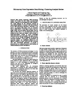
Fig. 1: Expression Matrix showing a single bi-cluster. Genes are represented as rows and columns are represented as columns. Elements of bi-cluster are highlighted in bold.

( {I, 2, 5, 7}, {I, 6, 8} ) is defined. The bi-cluster is represented in such a way that the bi-cluster consists of genes gl,g2,g5,g7 and conditions Cl,C6,CS. The size of the bi-cluster (volume) is 12. The important parameters to measure the quality bi-clusters is described below: 1) Let a bi-cluster be represented as squared residue of a bi-cluster P x

msrpq

P Q. The mean Q is defined as: x

1

=

2..: msr�q IPI.IQI pEPqEQ

(1)

where

msrpq

=

Xpq-xpQ -XPq

+

xPQ

Eqn. (1) represents the mean squared residue of a bi­ cluster P x Q, msrpq represents the residue of an element Xpq of P x Q. xpQ represents mean row, XPq represents mean column and xPQ represents mean of all entries in P x Q. The smaller the mean squared residue of a bi-cluster, the better the homogeneity of the bi-cluster. The other important parameter that discards trivial bi-clusters is the row variance. 2) Row variance of a bi-cluster P x Q is defined as:

BI-CLUSTERING

variancepQ

The basic concept to form a bi-cluster is described in [1]. Let the set of genes be represented as G {gl,g2,... ,g!vI } and the set of conditions be denoted as C {Cl' C2,... ,CN }. The expression matrix (EM) can be represented as a matrix of size Ai[ x N where each entry of EM is denoted by Xij. A bi-cluster is a sub-matrix P x Q, where P is a subset of M and Q is a subset of N, that shows high similarity of behaviours. The homogeneity of a bi-cluster P x Q is defined by mean squared residue and the volume of a bi-cluster is defined as number of elements Xij present in the bi-cluster. Consider the example in Fig. 1. Let us assume that seven genes and eight conditions make up an EM i.e. 7 x 8 where rows of EM correspond to genes and columns of EM correspond to conditions. In this figure, a bi-cluster =

=

1 2..: variancepq P I I.IQI pEPqEQ

(2)

Relatively large row variance is preferred as it improves the goodness of bi-cluster.

=

The main objective of this paper is to find bi-clusters having large volume i.e. maximal subsets of genes showing highly coherent behaviour under maximal subsets of conditions. To achieve this objective, MSR value should be less and row variance value should be relatively larger. IV.

GENETIC ALGORITHM

A. Sequential Genetic Algorithm GA is a powerful search technique which is used to derive bi-clusters of maximum size. The exploration of search space

978-1-4673-6540-6/15/$31.00 ©2015 IEEE

2

where M represents number of rows and N represents number of columns, Xpq represents an entry in the EM. 1Cov ( xpq ) 1 represents the number of chromosomes in the cell array BiclusterStore covering an element Xpq. By adjusting weight of each element in EM, the search can be controlled to focus on bi-clusters that are not yet found. The goal of the method callGA( ) is to search for best bi-clusters that have mean squared residue less than 6 and to return to Biclustering Algorithm. 1) Binary encoding of chromosomes: Each chromosome of the population represents one bi-cluster. Binary encoding is used to encode the bi-clusters. The length of the bi-cluster is M + N where M corresponds to number of rows and N corresponds to number of columns of the EM. The beginning M bits of the binary string represents the number of genes and the rest N bits represents the number of conditions [1]. Consider an example to understand the encoding of a bi-cluster (shown in Fig. 1). The bi-cluster can be binary encoded as shown below:

and exploitation of solutions are greatly controlled by two pa­ rameters such as probability of crossover (Pc) and probability of mutation (Pm). The steps involved to derive biclusters are shown below in Fig. 2.

Fig. 2: Bi-clustering using sequential GA

1 100101110000101 The length of the encoded binary string of the bi-cluster is 15 where first seven bits represent genes and last eight bits represent conditions. For marking the bits of the genes and the bits of the conditions, a symbol 1 is used. By setting any two bits randomly to I, the bi-clusters in the initial population contains only one element. The rest of the bits in the binary string is set to zero. 2) Fitness Function: Fitness function is a measure of the objective function. The fitness value summarizes, how close a candidate solution is towards achieving its objective. In this problem, the fitness value of every chromosome can be evaluated using the following equation:

Fig. 3: Steps of method callGA( )

. j(E)

The first figure (Fig. 2 (a)) invokes GA as a function (callGA( )). The execution of callGA( ) continues till the stopping criteria is met (shown in Fig. 2(b)). Once the stopping criteria is met and the process terminates, the mean squared residue of the best individual in the population is compared with 6. If the mean squared residue is less than 6, then the bi-cluster is returned to Fig. 2 (a) otherwise the bi-cluster is not returned. The method callGA( ) is called many times till stopping criteria is met. The bi-clusters found by callGA( ) are stored in a cell array BiclusterStore and to escape from overlapping among sub­ matrices, weight of each element in the EM is updated. The number of times an element is covered by the bi-clusters in the cell array BiclusterStore, the weight of an entry in the EM depends on it. If an element is covered by many bi-clusters in the cell array BiclusterStore, then the weight of the element will be very large as suggested in [1]. The weight 11ib of an entry Xpq of the EM is updated as per the following conditions:

residue(E)

6

=

if

ICov(xpql ICov(xpql

=

+ 11id +

penalty (4)

where E represents an individual, mean squared residue of an encoded bi-cluster is represented by residue(E) and row variance of the individual is represented by variance(E). Maintaining diversity in the population is also an important aspect in evolutionary algorithm. Thus, the parameter penalty is added in the objective function so as to allow other less similar bi-clusters to remain in the population. The penalty parameter avoids the redundant bi-clusters to get selected in the subsequent generations. The concept of penalty parameter is described in [1] and represented in the equation below:

penalty

=

11ib ( Xpq )

L

(5)

pEP,qEQ

where P and Q correspond to the rows and columns of a bi­ cluster respectively. Eqn. 3 defines wb. The definition of 11id is also taken from [1] and is defined as: 11id

if

1 vaT"tanCe(E)

.

+

0

=

11iv ( 11ir

•

6/ r011ix

+ 11ie

•

6/ colx)

(6)

To give more or less significance to the size of the bi­ cluster, 11iv is used and the default value of 11iv is set to one.

> 0

(3)

978-1-4673-6540-6/15/$31.00 ©2015 IEEE

3

The weights assigned to the number of rows and number of columns are determined by Wr and We respectively and rowx and calx represents the number of rows and columns of the encoded bi-cluster respectively. To trade off the influence of the large number of genes to small number of conditions in Eqn. 4; Eqn. 5 is empirically found. Considering Eqn. 4, if 5 > residue(E), the value of residue(E) . . . IS Iess than 1. If row vanance IS Iarge, then b 1 r071Jvartance(E) is a small value. obtained. To get the best quality of bi-clusters, the residue(E) should be small than 5 and the rowvariance(E) should be as large as possible. The best bi-cluster has the smallest fitness value. 3) Genetic Algorithm Operators: The genetic algorithm has three types of operators: selection. crossover and mutation.

Algorithm 1 Coarse grained Parallel Genetic Algorithm with migration Input: Threshold 5, MigrationInterval Output: Bi-clusters having mean squared residue less than a given 5 Step 1 Load Expression matrix (EM) Step 2 Specify the number of cores to be used in parallel (for e.g. matlabpool(open. 4) specifying that four cores will be used) Step 3 for GenerationNumber 1 to maxgeneration do %% execute each generation in four cores in parallel Step 3.1 initialize population Step 3.2 evaluate population Step 3.1 initialize count to 0 Step 3.4 for (GenerationNumber j 1 to maxgeneration) do Step 3.4.1 count++ Step 3.4.2 select parents Step 3.4.3 crossover each pair of parents Step 3.4.4 mutation of resultant offsprings Step 3.4.5 evaluate new individuals Step 3.4.6 select survivor individuals for next genera­ tion Step 3.4.7 if (count M igrationInterval) then migrate the best individual of source deme and replace those individuals with the worst individuals of destination deme Count 0 end if end for Step 3.5 best...:individual best individual in each deme Step 3.6 finalBest...:indi select the best one from

1) Selection: Tournament selection operator is used. The tournament size is user-defined and the default size is 2. 2) Crossover: Two-point crossover method is used. 3) Mutation: Mutation is perfonned by flipping a bit i.e. setting a one bit to zero and vice versa. Mutation operator is applied in such a way that bi-cluster should be maximized. B. Parallel Genetic Algorithm Standard GA has been successfully used to solve various types of problems. But the major issue lies in the convergence speed, as GA takes too long time to converge if the size of the population increases. Parallel GA (PGA) can efficiently handle the major problem encountered by traditional GA. The partition of population into some number of demes (sub­ population) is required in PGA. The basic concept of PGA is described in [18]. In this paper, Coarse grained Parallel Genetic Algorithm with Migration is used. This framework is a deme structure having relatively small number of sub-population with large number of individuals. The application of PGA to solve the bi-clustering problem is described in [15]. The encoding of bi-clusters is same as defined for traditional GA. Fitness function for CgPGA is also same as GA. Genetic Operators are executed in parallel at multiple processors. Sev­ eral number of parameters control the migration of individuals from one sub-population to another. These parameters are described below:

==

=

=

=

besCindividual Step 3.7 if residue (jinalBesCindi) < 5 then return the bi-cluster finalBesCindi end ifStep 3.8 if (bicluster found) then store bi-cluster in BiclusterStore and update weights of each element in EM else do nothing end if end for Step 4 return BiclusterStore

1) A topology should be defined to communicate among the sub-populations, e.g. 2D/3D mesh, hypercube, torus, ring etc. 2) The number of individuals to be migrated is restricted by migration rate. 3) A migration scheme controls which chromosome from the source sub-population (best, random, worst) should be migrated to another sub-population, and which chro­ mosomes should be substituted (worst, random, best) 4) The number of times migration should be performed is determined by migration interval. Proposed Algorithm: The detail steps of CgPGA with migration is described below.

978-1-4673-6540-6/15/$31.00 ©2015 IEEE

4

V.

NUMERIC AL SIMUL ATION RESULTS AND DISCUSSION 15000

The algorithms for sequential GA and CgPGA are imple­ mented using Matlab R2009B and it was executed on Lenovo ideapad Z580 intel core i3 with 4GB of RAM. Only four cores, being two virtual cores, were available to work in parallel. The appropriate values for Wr 1 and We 10 were assumed. In tables shown below (Table I and II), Wt represents weight. The experiments were performed on well-known dataset that is yeast Saccharomyces cerevisiae cell cycle expression data set from http://arep.med.harvard.edulbi-clusterl. The dataset consists of 2,884 genes and 17 experimental conditions. The preprocessing of the original matrix was done using the following min-max normalization so that every value of EM falls within the range of 0 to l. =

.

. '

x(Z,] )

=

x(i,j)-colmin colmax -COlmin

:

A",,,ge Volume

X 10

•

BeslVolume

E EJ E]

10000

5000

D

=

EJ

O

50

100

t

as

0

0

50

100

Fig. 5: Graph showing average volume and best volume every generation.

1000

'DO BOO 700 600

(7)

A",,,ge Re"due

III

Lowest Residue

1000

BOO 600

400

200

0

50

100

0

0

50

lOa

The parameter values assumed for sequential GA and CgPGA are shown below in Table I and II.

Fig. 6: Graph showing average mean squared residue and lowest mean squared residue in every generation.

TABLE I: Parameter values for sequential GA

TABLE III: Information about bi-clusters found by Sequential GA

Parameter name

Value

Population size Nmnber of generations Probability of crossover Probability of mutation Wt for conditions Wt for genes Number of genes taken Threshold J

50 100 0.50 0.20 10 I 10 800

Gen. No. 9 12 13 20 21 26 34 35 36 37 44 45 48 49 50

TABLE II: Parameter values for CgPGA

2

500

2000 1500 1000 500

Parameter name

Value

Population size Number of generations Probability of crossover Probability of mutation Wt for conditions Wt for genes Number of genes taken Threshold J

50 50 0.50 0.20 10 1 500 800

A"",eF II O'"

Gen. No. 2 9 10 14 15 19 20 21 28 32 33 35 40 42 44 45 46 47

BestFitness

BOD

600

0

50

100

4 ° 0

0

50

Col. 13 3 2 4 4 4 1 4 5 3 1 4 4 6 4

Vol. 3298 749 474 901 922 663 245 685 1290 658 251 971 972 1228 656

Row Var. 812 639 719 832 798 725 0 487 858 657 0 576 741 883 602

Fit. value 1.0e+008* 0.0000 0.1404 0.0629 0.1654 0.1511 0.1214 0.0428 0.4612 0.7875 0.5026 0.5213 0.6380 1.3427 2.3377 1.5615

TABLE IV: Information about bi-clusters found by CgPGA

00 1000

Rows 265 260 247 240 237 237 259 243 267 236 272 261 256 257 226

100

Fig. 4: Graph showing average fitness and best fitness in every generation. From numerical simulation it was observed that, the execu­ tion time for sequential GA was very slow. For this reason, only 200 genes were considered in the experiment. The graphs shown in Fig. 3, 4 and 5 are the results obtained after the execution of the steps shown in the method callGA( ) over

978-1-4673-6540-6/15/$31.00 ©2015 IEEE

5

Rows 251 258 266 242 266 242 258 265 245 234 238 272 254 260 242 251 251 250

Col. 16 13 12 15 12 15 13 11 14 16 15 13 15 13 13 13 14 14

Vol. 3837 3190 3026 3456 2771 3798 3118 2758 2983 3296 3109 3120 3377 2956 3089 3078 3078 3111

Row Var. 852 869 749 870 830 854 739 795 821 821 842 821 873 815 804 780 780 858

Fit. value 1.0e+008* 504 619 670 538 731 576 619 731 619 538 576 670 575 670 619 619 619 619

yeast dataset using sequential GA. Sequential GA and CgPGA were implemented using parameters as specified in Table I and Table II respectively. The graphs are plotted after the first call to the method callGA( ). In Fig. 3, 4 and 5, horizontal axes represents subsequent generations and the vertical axes represents fitness value, volume and mean squared residue of each individual respectively. The result of CgPGA was quite efficient in terms of exe­ cution time, number of conditions that genes were responding to, the volume of the bi-clusters, and fitness value. If the fitness value of a bi-cluster is too low, then the quality of the bi-cluster is too high. The results of sequential GA and CgPGA are shown in Table III and Table IV respectively. After the execution of both algorithms, it was observed that sequential GA found 15 bi-clusters and CgPGA found 18 bi-clusters covering 38.98% of the cells in the EM, 50.5% of the genes, 80.7 % of the conditions with population size of 50. CgPGA derived larger volume bi-clusters at a faster rate considering 500 number of genes. The row variance of bi-clusters found by CgPGA are much larger as compared to sequential GA. The fitness value of the bi-clusters found by CgPGA is much smaller than the fitness value of the bi­ clusters found by sequential GA. Each generation of Step no. 3 of CgPGA, took 30 seconds while each call to the method callGA( )(shown in Fig. 2(b)) took 250 second�. SEBI returned 100 bi-clusters which covered 38.14% of the cells in the EM, it covered 43.55% of the genes, and 100% of the conditions with population size of 200. CgPGA took very less time to converge when compared with other existing algorithms.

[2] Sushmita Mitra and Haider Banka,"Multi-objective evolutionary bi­ clustering of gene expression data," Pattern Recognition ,Elsevier, vol. 39,pp. 2464-2477, 2006. [3] Cheng,Yizong,and George M. Church, "Biclustering of expression data," Ismb,Vol. 8. 2000. [4] Hongya Zhao, KwokLeungChan, Lee-MingCheng, and HongYan, "A probabilistic relaxation labelling framework for reducing the noise effect in geometric bi-clustering of gene expression data," Pattern Recognition, Elsevier, vol. 42,pp. 2578-2588, 2009. [5] Neelima Gupta and Seema Aggarwal, "MIB: Using mutual information for bi-clustering gene expression data," Pattern Recognition,Elsevier,vol. 43,pp. 2692-2697, 2010. [6] Jaegyoon Ahn, Youngmi Yoon, and Sanghyun Park, "Noise-robust al­ gorithm for identifying functionally associated bi-clusters from gene expression data,",Information Sciences,Elsevier, vol. 181,pp. 435-449, 2011. [7] B. Hanczar and M.Nadif, "Using the bagging approach for bi-clustering of gene expression data," Neurocomputing, Elsevier, vol. 74, pp. 15951605,2011. [8] K.O. Cheng, N.F.Law, and W.C.Siu, "Iterative bi-cluster-based least square framework for estimation of missing values in microarray gene expression data," Pattern Recognition, Elsevier, vol. 45, pp. 1281-1289, 2012. [9] Jose L. Flores, Inaki Inza, Pedro Larranaga, and Borja Calvo, "A new measure for gene expression bi-clustering based on non-parametric correlation," Computer methods and programs in biomedicine, Elsevier, vol. 112,pp.367-397,2013. [10] Fabrizio Angiulli,Eugenio Cesario, and Clara Pizzuti, "Random walk bi-clustering for microarray data," Information Sciences, Elsevier, vol. 178,pp. 1479-1497,2008. [11] Sushmita Mitra,Ranajit Das, Haider Banka, and Subhasis Mukhopad­ hyay, "Gene interaction - An evolutionary bi-clustering approach," Infor­ mation Fusion,Elsevier,vol. 10,pp. 242-249,2009. [12] Pedro Cannona-Saez, Roberto D Pascual-Marqui, F Tirado, Jose M Carazo,and Alberto Pascual-Montano, "Bi-clustering of gene expression data by non-smooth non-negative matrix factorization," BMC Bioinfor­ matics, vol. 7,2006. [13] Jochen Supper,Martin Strauch,Dierk Wanke,Klaus Harter,and Andreas Zell, "EDISA: extracting bi-clusters from multiple time-series of gene expression profiles," BMC Bioinfonnatics, vol.8,2007. [14] J.A. Hartigan, "Direct clustering of Data Matrix," Journal of the Amer­ ican Statistical Association,Vol. 67,pp. 123-129,1972. [15] Wei Shen,Guixia Liu,Ming Zheng Zhangxu Li,Yi Zhong,Jianan Wu, and Chunguang Zhou, "A Novel biclustering algorithm and its application in gene expression profiles," Journal of Information and Computational Science, vol. 9,pp. 3113-3122, 2012. [16] Kenneth Bryan, Padraig Cunningham, and Nadia Bolshakova, "Appli­ cation of Simulated Annealing to the Biclustering of Gene Expression Data," Ieee transaction of information technology in biomedicine, vol. 10,2006. [17] Melanie Mitchell, "An Introduction to Genetic Algorithms," a Bradford book The MIT Press ISBN,0262133164 (HB),0262631857 (PB),1996. [18] Mariusz Nowostawski and Riccardo Poli, "Parallel Genetic Algorithm Taxonomy," In proc. of Third International Conference on Knowledge­ Based Intelligent Information Engineering Systems,pp. 88-92,1999. [19] Guilherme Palenno Coelho,Fabricio Olivetti de Franca,and Fernndo J. Von Zuben, "A Multi-population Approach for Biclustering," Springer­ Verlag Berlin Heidelberg, pp. 71-82,2008. [20] c. Cano, L. Adarve, J. Lpez, A. Blanco, "Possibilistic approach for biclustering microarray data," Computers in Biology and Medicine, Elsevier, vol. 37,pp. 1426-1436,2007. [21] Jiang Daxin,Chun Tang,and Aidong Zhang, "Cluster analysis for gene expression data: A survey," IEEE Transactions on Knowledge and Data Engineering,vol. 16,pp. 1370-1386, 2004. [22] Hruschka E. R.,Campello R. J. G. B.,Freitas A. A.,and De Carvalho, A. P. L. F., "A survey of evolutionary algorithms for clustering," IEEE Transactions on Systems,Man,and Cybernetics,Part C: Applications and Reviews, vol. 39(2),pp. 133-155, 2009.

TABLE V: Comparative study on Yeast data Algo. used Sequential GA CgPGA Cheng-Church FLOC SEBI

Avg.

MSR 653 755 204.29 187.54 205.18

Avg. volume 930.8 3175 1576.98 1825.78 209.92

VI.

Avg. no. of genes 250.87 252.5 167 195 13.61

Avg. no. of columns 4.13 13.72 12 12.8 15.25

CONCLUSION

From numerical simulations, it is observed that CgPGA has outperformed traditional GA in terms of execution time. The size of the bi-clusters obtained from CgPGA is larger in size as compared to traditional GA. The homogeneity of the bi­ clusters might not be the best compared to other results, but CgPGA was successful in getting the larger size of bi-clusters which means more number of genes were exhibiting more similar behaviours over same subset of conditions. Therefore, CgPGA was successful in deriving high quality bi-clusters compared to existing techniques. Work can be further extended to implement some other variations of PGA to further improve the quality of bi-clusters. REFERENCES [1] Federico Divina and Jesus S. Aguilar-Ruiz, "Bi-clustering of Expression Data with Evolutionary Computation ", ieee transactions on knowledge and data engineering,vol. 18,no. 5,2006.

978-1-4673-6540-6/15/$31.00 ©2015 IEEE

6