May 27, 2005 - Part of the Lecture Notes in Computer Science book series (LNCS, volume 715). Cite this ... In: Best E. (eds) CONCUR'93. CONCUR ... On leave from The School of Mathematics and Computer Science, Tel Aviv University.
B i s i m u l a t i o n Equivalence is Decidable for Basic Parallel Processes Scren Christensen
Y o r a m Hirshfeld*
F a r o n Moller t Laboratory for Foundations of Computer Science University of Edinburgh
Abstract In a previous paper the authors proved the decidability of bisimulation equivalence over two subclasses of recurslve processes involving a parallel composition operator, namely the so-caUed norrned and live processes. In this paper, we extend this result to the whole class. The decidability proof permits us further to present a complete axiomatisation for this class of basic parallel processes. This result can be viewed as a proper extension of Miiner's complete axiomatisation of bisimulation equivalence on regular processes.
1 Introduction Finite-state systems have been extensively studied, both within standard formal language theory and within the theory of process calculi. Certainly all standard behavioural equivalences, in particular those within the linear time-branching time spectrum of [8], are decidable over finite-state systems, and complete aadomatisations have been developed for various of these equivalences between them (see, eg, [22, 18, 16]). Furthermore, there have been many automated tools designed for the analysis of such systems (see, eg, [17]). Recently, questions regarding the decidability of process equivalences on various classes of infinite-state systems have been studied. Certainly when we move to contextfree processes, language equivalence becomes undecidable. However, of greater interest in process theory are questions regarding stronger notions of equivalence which take into account for instance the notions of deadlock, livelock, or causality. In [14, 10] it is demonstrated that all of the standard behavioural equivalences besides bisimflarity are undecidable over context-free processes. However in [7] it is shown that bisimilarity is in fact decidable over this class of infinite-state processes. Previous to this, there were several proofs of this result for the subclass of normed processes, those processes which may terminate in a finite number of steps at any point during their execution ([1, 3, 13, 9]). *On leave from The School of Mathematics and Computer Science, Tel Aviv University. tSupported by ESPRIT BRA 7166: CONCUR2.
144
The class of context-free processes is provided by a standard process calculus which admits of a general sequencing operator, along with atomic actions and choice. However Of greater importance in process theory is the inclusion of some form of parallel combinator. Very little work it seems has been spent on exploring the decidability (or otherwise) of equivalences defined over process calculi which include parallel combinators within recursive definitions. Certainly with very little else you can express the full power of Turing machines along with their undecidable problems [i9]. In [6] we explored a calculus which i n c l u d e s a simple parallel combinator. We showed that in the case of normed processes, and also for live processes (processes which can never perform an infinite number of identical actions in succession uninterrupted), we can prove decidability of bisimulation equivalence. In order to obtain our results, we required cancellation laws for normed and live processes. Such a law is not valid over the whole calculus, so the proof technique presented there is not valid in general. In this paper, we demonstrate a refinement of the argument presented in [6] which settles the decidability of bisimulation equivalence over the whole calculus. As with [6], the technique which we use to provide the decidability result is based on the use of tableau systems. From the rules we present for generating our tableaux we can extract a sound and complete equational theory for our calculus. As our class of processes clearly contains the regular processes this result can be viewed as a proper extension to Milner's equational theory of bisimulation equivalence on regular processes [18].
2
Preliminaries
We presuppose a countably infinite set of atomic actions A = {a, b, c,...} as well as a countably infinite set of process variables Vat = {X, Y, Z , . . . } . The class of recursive BPP (Basic Parallel Processes) expressions is defined by the following abstract syntax equation. E
::= 0 ] X
I aE I E + E
t EHE
(inaction) (process variable, X E Var) (action prefix, a E A) (choice) (merge)
We shall omit trailing 0s from expressions, thus writing the term a0 simply as a. Also we shall write E = to represent the term E l l . . . lIE consisting of n copies of E combined in parallel. A BPP process is defined by a finite family of recursive process equations
= {x, "~ E, j where the X i are distinct and the E i are BPP expressions at most containing the variables Vat(A) = { X l , . . . , X~}. We further assume that every variable occurrence in the E~s are guarded, that is, appear within the scope of an action prefix. The variable Xx is singled out as the leading variable and X 1 = Ex is called the leading equatior~ Any finite family A of BPP equations determines a labelled transition system. The transition relations are given as the least relations satisfying the following rules.
145
b
a.o/. ~'~
b
~'J'~
b
~'~
b
Figure 1: The transition graph for {X a___ca(X]lb)}. f
aE --~ E
E - - ~ E' E + F _2_. E'
E ~ E' _ BilE --~ E'HF
E --~ E I ~ E X --~ E' ( Z E A)
F -~ FI Z + F - ~ F'
F --% F I EHF ~ EIlF'
Strictly speaking, transitions are defined on BPP expressions relative to some family A of process equations. However, we shall usually leave the reader to infer the intended family. R e m a r k 2.1 It is easy to verify that BPP processes generate finite branching trans-
ition graphs, that is, graphs for which the se~ {F : E --~ F} is finite for each E and each a. This would not be true if we allowed unguarded expressions. For example, the process X d_e_fa + al[X generates an infinite-branching transition graph. R e m a r k 2.2 For the purpose of this presentation, we only consider pure merge for our
parallel combinator. However, it is easily seen that the results of this paper hold (with the obvious slight modifications) if we allow handshake communication in the style of CCS. Hence the calculus we are considering is (guarded) CCS without restriction and relabelIing. In order to simplify our later analysis, we wish to identify several process expressions. A typical case is that we want ]1to be commutative and associative. We therefore define the following structural congruence over process expressions. D e f i n i t i o n 2.3 Let -
be the smallest congruence relation over process expressions such that the laws of associativity, commutativity and O-absorption hold for choice and merge.
When inferring transitions we may ignore harmless 0-components sitting in parallel. Thus not to be annoyed by such innocent matters we shall always assume that transitions have been inferred modulo the structural congruence -=. We note that we can safely do so since the semantic equivalence of bisimflarity (which we introduce shortly) satisfies the basic laws underlying the structural congruence =. E x a m p l e 2.4 Let A be the family { X ~ a(XIIb)}. By the transition rules above
(modulo - ) X generates the infinite-state transition graph of Figure 1. The equivalence between BPP expressions (states) which we are interested in considering here is bisimilarity [19], defined as follows.
146
D e f i n i t i o n 2.5 A binary relation 7r over BPP expressions (states) is a bisimulation if whenever E ~ F then for each a E A,
9 if E --~ E ~ then F -2-* F' for some F' with E'TCF~; 9 if F --~ F I then E _.L. E' for some E ~ with E'TCF'. Processes E and F are bisimilar, written E ,,~ F, i.f they are related by some bisimulation. By Vat(A) | we denote the set of finite multisets over Vat(A) -- { X i , . . . , X , } and let Greek letters a, fl . . . . range over elements of Vat(A) | Each such a denotes a BPP process by forming the product of the elements of a, i.e. by combining the elements of a in parallel using the merge operator. We recognise the empty product as 0, and we ignore the ordering of variables in products, hence identifying processes denoted by elements of Vat(A) | up to associativity and commutativity of merge. D e f i n i t i o n 2.6 A finite family A = {Xi ~ El [ 1 < i < n} of guarded BPP equations is defined to be in standard form iff every expression E i is of the form alo/1 q- ... -[-
area m
where for each j we have a i E Var(A) | Again, we recognise the empty sum as O, and ignore the ordering of expressions in sums, hence defining the notion of standard form modulo associativity and commutativity of choice. In [19] it is shown that any finite family A of guarded BPP equations has a unique solution up to bisimilarity. Moreover, in [5] we have the following result showing that any such system can be effectively presented in standard form. L e m m a 2.7 Given any finite family of guarded BPP equations A we can effectively construct another finite family of BPP equations A' in standard form in which A ,,, A I, i.e. the leading variables of A and A J are bisimilar. For our proof of decidability of bisimulation equivalence we shall rely on the following ordering on Vat(A) | D e f i n i t i o n 2.8 By E we denote the well-founded ordering on Vat(A) | given as follows:
X~'ll... II~" E x['ll... IIX~ iff there exists j such that kj < lj and for all i < j we have k i = 1i. It is straightforward to show that E is well-founded. We shall furthermore rely on the fact that E is total in the sense that for any a, fl E Var(A) | with a ~ fl it follows that a E fl or fl E a. Also we shall rely on the fact that ]~ E a implies ]~]['r E a[[*/for any 7 E Vat(A) | These properties are easily seen to hold for E.
147
3
Decidability
In this section we fix a finite family A = {Xi ~ t E/ I 1 < i < n} of guarded BPP equations in standard form. We are interested in deciding for any a and fl of Vat(A) | whether s ,-,/3 is the case or not. The procedure for checking s ,~/3 is based on the tableau decision method as for instance utilised by Hiittel and Stirling in [13]. The tableau system is a goal directed proof system. The rules of the tableau system are built around equations E = F where E and F are BPP expressions. Each rule has the form E=F El=El
...
E.=F.
possibly with side conditions. The premise of the rule represents the goal to be achieved (that E ,-, F ) whereas the consequents represent (sufficient) subgoals to be established. A tableau for c~ = 3 is a maximal proof tree whose root is labelled a = fl and where the labelling of immediate successors of a node are determined according to the rules of the tableau system presented in Table 1. For the presentation of rule REC we introduce the notation unf(s) to mean the unfolding of s defined as follows: given Y/ ---- ~ i =R4l aijsij for 1 < i < m, ~i
~rt
unf(Y:tll' " flY,,,) = Z ~ a,j(Ydl - IIY~-llls,jilY~+dl" " IIY,r,). i=l 3"=1
We shall identify BPP expressions in our tableaux up to the structural congruence =, i.e. up to associativity, commutativity and 0-absorption of choice and merge. In particular, we always assume that the labels of nodes have been pruned of 0 components sitting in parallel or in sum; rule REC might introduce such innocent components. We adopt some terminology for tableaux. Tableaux are denoted by T (and also by T ( a = 3) to indicate the label of the root). Paths are denoted by 7r and nodes are denoted by n (with roots also denoted by r) possibly with subscripts. If a node n has label E = F we write n : E = F. In building tableaux the rules are only applied to nodes that are not terminal. A terminal node can either be successful or unsuccessful. A successful terminal node is one labelled s = s, while art unsuccessful terminal node is one labelled either a s = bfl such that a ~ b or a s = 0 or 0 = b/L A tableau is successful if and only if all terminal nodes are successful; otherwise it is unsuccessful. Tableaux are built from basic steps. A basic step for a = 3 consists of an application of REC to s = / 3 followed (possibly) by an application of SUM followed by an application of PREFIX to each of its consequents. See Figure 2 for the schema of a basic step. A ~=~
REC Eaioti=Ebi~i SUM
anal
= blfll
a.a.
= b.~.
PREFIX
PREFIX a~ = 3~
a . = 3.
Figure 2: A basic step.
148
REC
unf(c~) -- unf(,6) ~vt
SUM
b where f : {1,... ,n} --~ {i. . . . . m} 9: { l , . . . , m } ~ {1,...,n}
PREFIX
ac~ = a~ c~=(3 ~lFf =
SuBL
SUBR
if the dominated node is labelled
c~= ~ or ~ = c~ with c~ D fl
if the dominated node is labelled c ~ = ~ or ~ = a with c~ ~ fl
Table 1: Rules of the tableau system. basic step represents a set of single transition steps in the operational semantics: for each consequent al = fll we have a - ~ al and ~ - - ~ fl~. Nodes of t h e form n : a = fi are called basic nodes. W h e n building t a b l e a u x basic nodes m i g h t dominate other basic nodes; we say a basic node n : ~llh' = 6 or n : 6 = a]] 7 d o m i n a t e s any node n ~ : a = ~ or n ' : fl = a which appears above n in the t a b l e a u in which a -1 j3 a n d to which rule REC is applied. W h e n e v e r a basic node dominates a previous one, we apply one of the SUB rules to reduce t h e t e r m s before applying t h e REC rule. Notice t h a t the side condition for t h e SUB rules is a condition on t a b l e a u x a n d not on the particular rule. E x a m p l e 3.1 Let { X 1 d=da(XllIX4),X2 ~ f a X 3 , X 3 d-~--fa(X~]IX4) + b X 2 , X a ~( b} be a family of B P P processes in standard form. In Figure 3 we give a successful tableau for X 1 = X 2. Notice that these processes are neither normed nor live, so the techniques described in [6] are inapplicable. 3.2 Every tableau for a = ~ is finite. Furthermore, there is only a finite number of tableaux for a = ,8.
Lemma
P r o o f : Let T ( a -- fl) be a tableau with root labelled a = ft. It can only b e infinite if there exists a n infinite p a t h as every node has finite b r a n c h i n g degree. Hence suppose ~r is such a n infinite p a t h starting at the root r : a = ~. The p a t h ~r can only be infinite
149
X1= X2
REC
a(Xl IIZ~) = aX~
PREFIX
SUBL REC SUM PREFIX
x~ IIX, = x , X2[iX4 =
.(X, tlX,)+ bx~ =
X3
. ( X , llX,) + bX~
a(XaIIX4) = a(Xa [IX,)
bX2 = bX2
x~llx, - XallX~
x~ - x2
PREFIX
Figure 3: A successful tableau for X 1 = X 2.
if it contains infinitely many basic nodes to which the tableau rule REC is applied. This is due to the well-foundedness of the ordering r" on V a t ( A ) | which is decreased through applications of the SUB rules. Thus from the path r we can form an infinite sequence S of nodes {r~ : a~ = fi~}~=l by collecting (in order of appearance) the basic nodes along ~r to which the rule P~Ec is applied. Hence n 1 : a 1 = ~1 represents the root, n 2 : a2 = ~2 represents the second node along n at which REC is applied, and so on.
An expression a can be viewed as a vector fi of/N~: the value of the i *h coordinate of ~, denoted ~(i), indicates the number of occurrences of variable Xi in a. Thus we can represent the sequence S by an infinite sequence of vectors {ui)i~l where fii 6 / N 2~ for all i. The first n coordinates represent a i and the last coordinates represent ~i. Consider the infinite sequence {fii(1)}~l consisting of all the first coordinates of vectors of the sequence S. If this sequence has an upper bound we extract from S an infinite sequence S1 of vectors {%1}i~=1with the property that the first coordinate of vl remains constant throughout $1. If the sequence {fii(1)}i~1 does not have an upper bound we extract from S an infinite sequence $1 of vectors {%i}i~l with the property that the first coordinate of ~i is nondecreasing, i.e. ~i(1) < %j(1) whenever i _< j. Continuing in this fashion we arrive at an infinite sequence $2~ of vectors {~'}i~1 with the property that all coordinate sequences are nondecreasing. But then every node in this sequence is dominated by every node after it, so the rule P~Ec cannot be applied to any of these nodes, as a SUB rule is applicable. For the proof of the second part, we note that if there were an infinite number of tableaux, then since there are only a finite number of tableaux of a given finite size, there must be an infinite sequence of partial tableaux, each of which being derived from the previous by the application of some rule to the node most recently introduced. But then this sequence provides a tableau with an infinite path through it, which by the first part cannot be. [] We now proceed to show the soundness and completeness of the tableau system. T h e o r e m 3.3 ( C o m p l e t e n e s s ) I f a ,,~ fl then there exists a successful tableau with root labelled a = ft.
P r o o f : Suppose a ~ ft. If we can construct a tableau T ( a = ~ ) for ~ = fl with the property that any node n : E = F o f T ( ~ = fl) satisfies E ~ F, then by Lemma 3.2 that
150 construction must terminate and each terminal will be successful. Thus the tableau itself will be successful. We can construct such a T ( ~ = ~) if we verify that each rule of the tableau system is forward sound in the sense that if the antecedent as well as all nodes above relate bisimilar processes then it is possible to find a set of consequents relating bisimilar processes. It is easily verified that the rules are indeed forward sound in this sense. Notice in particular that the rule REC reflects the expansion law for merge [19] and that forward soundness of the SUB rules follows "from the fact that bisimilarity is a congruence wrt merge. D The proof of soundness of the tableau system relies on an alternative characterisation of bisimulation, viz. as a sequence of approximations. co
D e f i n i t i o n 3.4 The sequence of bisimulation approximations { ~}~=o is defined inductively as follows. 9 E "~o F for all processes E and F ; 9 E "%+1 F ill for each a E A, - if E _2., E I then F - - ~ F I for some F' with E' ,,~ F'; - if F - - ~ F I then E ~
E I for some E I with E I ,,% F t.
It is a standard result (see for instance [19]) that for finite branching transition graphs, bisimulation is given as the limit of the above approximations:
n=0
As noted in Remark 2.1, BPP processes are finite branching~ T h e o r e m 3.5 ( S o u n d n e s s ) If there is a successful tableau for c~ = fl then c~ ,,,/3. P r o o f : Suppose T ( a = fl) is a tableau for a = fl, and that a ~/3. We shall construct a maximal path ~r = {n~ : El = Fi} through this tableau starting at the root a = ~ in which E i ~ F i for each i. Hence the terminal node of this path cannot be successful, so there can be no successful tableau for a = ft. While constructing ~r, we shall at the same time construct the sequence of integers {ml : El ~m, Fi and Ei " i F~ for all j < m~}. We shall also prove along the way that this sequence is nonincreasing, and strictly decreasing through applications of the rule PREFIX. Given n i : Ei = F i and mi, we get ni+1 : Ei+l = Fi+t and mi+ 1 according to the following cases: 9 If REC is applied to n/, then the consequent is n~+l and mi+l = ml. 9 If SUM is applied to n/, then there must be some consequent n/+ 1 : E~+1 = F~+1 with El+ t ~ , ~ F~+1 and E~+ 1 ~ j Fi+ 1 for all j < m~, so m~+ 1 = m i. 9 If PREFIX is applied to n/, then the consequent is n/+ 1 and mi+ 1 = m~ - 1.
151
* If SuBL is applied to ni : Ei = Fi then E i = Fi must be of the form atl 7 -- 6 with dominated node nj : a =/~ (a "7 ~). Since between nj and ni there must have been an intervening application of the rule PREFIX, we must have that m i < mj. We take the node r~+l : ~3117= 6, and show that we have some valid m~+l