May 13, 2007 - for the degree of Bachelor of Science(BSc.) Supervisor: Prof. ... Blind Source Separation, also known as BSS in the short form, is a method of recover- .... where f(x1,y2) is the joint pdf of x1 and y2, which are samples of X and Y taken at times ..... Cocktail party effect â wikipedia, the free encyclopedia, 2006.
Blind Source Separation: Recovering Signals from Mixtures An Investigation on Acoustic Localization by Time-Delay Estimation
A Thesis Written by Alexandra Craciun in partial fulfillment of requirements for the degree of Bachelor of Science(BSc.)
Supervisor: Prof. Mathias Bode
Jacobs University Bremen gGmbH May 13th 2007
Contents 1 Abstract
2
2 Introduction
2
3 Implementation 3.1 General model . . . . . . . . . . . . . . . . . . 3.2 Simple case scenario . . . . . . . . . . . . . . . 3.3 Random Signal Sources . . . . . . . . . . . . . 3.4 Noise Considerations . . . . . . . . . . . . . . . 3.5 Real Audio Signals Simulations . . . . . . . . . 3.6 Audio Files with Additional Noise and Distance 3.7 Space Localization . . . . . . . . . . . . . . . . 4 Conclusions and Future Developments References
. . . . . . . . . . . . . . . . . . . . Decay . . . .
. . . . . . .
. . . . . . .
. . . . . . .
. . . . . . .
. . . . . . .
. . . . . . .
. . . . . . .
. . . . . . .
. . . . . . .
. . . . . . .
. . . . . . .
5 5 5 9 9 10 14 16 18 18
1
1
Abstract
This paper presents a time-delay approach to Blind Source Separation (BSS). As settings, we consider a certain number of microphones, each receiving artificial mixtures of delayed signals. With the use of cross-correlation, the time delay between the signal sources is being estimated. Furthermore, the paper investigates the possible localizations of the sources, while taking into consideration geometrical scenarios. Noise additions also make part of a series of experiments, on the basis of which the effects introduced by distortions are being analyzed. In addition, a specific real-world case is examined, for which we try to obtain the best performance and also derive the acoustic localization based on delay estimations.
2
Introduction
Blind Source Separation, also known as BSS in the short form, is a method of recovering signals from mixtures. The term ’blind’ means that there is no a-priori information regarding the original sources that could help us to identify them easier. The separation of sound sources is of great importance nowadays and BSS has attracted the attention of many researchers in an attempt to solve the noise or reverberations problem which often appears in recording systems, but not only. The diversity of its utilization is quite large and while playing a key role for hearing aids and structured audio coding, it has brought vast improvements in medicine, where it is of particular use for EEG (electroencephalogram), MEG (magnetoencephalogram) or fMRI (functional magnetic resonance imaging). However, apart from being very important for accurate medical diagnosis, BSS is applied also in telecommunication systems - for example in separating voice from noise in mobile phone conversations - or in speech recognition devices. Together with the rapid technological advancement, more and more accurate results are required and as a result, better and faster algorithms need to be implemented in order to solve the BSS problem. An interesting, yet still under research situation is the so-called ’Cocktail Party Effect’, or the ability to concentrate someone’s attention to a single talker among a mixture of other conversations, as well as background noises. This certainly reveals the extraordinary capacities of our auditory system, which allows us to quickly suppress any undesired sources, while enhancing the signal we are interested in hearing. In the 1950s, Donald Broadbent conducted a series of experiments on dichotic listening, where subjects were asked to hear and separate different speech signals presented to each ear simultaneously (using headphones). From the results of his experiment, he suggested that our ”mind can be conceived as a radio receiving many channels at once”: the brain separates incoming sound into channels based on physical characteristics (e.g. perceived location), and submits only certain subsignals for semantic analysis (deciphering meaning). In other words, there exists a type of audio filter in our brain that selects which channel we should pay attention to from the many kinds of sounds perceived[6]. The motivation behind this paper is to understand better the mechanisms behind BSS theory and see if indeed, there are particular characteristics of the mixtures that we can use to subtract the original sources. One of the many existing approaches considers the time-space relation, which can be derived from the mixtures themselves. More precisely, a mixture of signals can be seen as a linear combinations of delayed versions of the original audio sources.
2
A simple interpretation of the previous idea regards a number n of sources s1 (t), s2 (t), . . . , sn (t) as the signals sent to a series of microphones placed at certain distances from the sources. Each microphone would then receive a mixture of the following form: mi = αi1 s1 (t − ti1 ) + αi2 s2 (t − ti2 ) + . . . + αin sn (t − tin )
(2.1)
Variables tij represent the time it takes for signal from source j to arrive at microphone i. The coefficients α1 , α2 , . . . , αn are the ratio by which the signal is reduced as a function of time. Since the higher the delay is, the larger the distance between transmitter and receiver becomes, when the signal finally reaches the microphone, it will have a smaller amplitude, depending on what distance it traveled. For the sake of simplicity, we consider for almost all of the simulations the α’s to be 1 (if not stated otherwise). By finding out the amount of delay with which a signal reaches the microphone, the distance between the two can be calculating, knowing that: c = 331 + 0.6T [m/s]
(2.2) o
where c is the speed of sound. At normal temperature (' 20 ), the speed of sound is approximately 343 m/s. As an example, if we knew that source x reached microphone y with a delay t of 1 second, that would correspond to a distance of d = c · t = 343m/s · 1 = 343m
(2.3)
The simulations made for this paper are however intended to recreate a closed environment (room, car, etc.). Therefore, a distance of 343 m is unrealistic in this scenario. We would rather prefer a distance ranging between 0.2m and 2m, which means having delays from 0.58 to 5.83 msec. A problem appears when we want to find out the actual delays since we don’t know exactly which delay corresponds to which source. All we have are different mixtures received at the microphones, so we have to come up with a solution of deriving at least a relationship between the delays for each source reaching microphone i. One way to do this is to use the cross-correlation on the mixtures we have at 2 microphones. Cross-correlation has been explained from two different points of view, one being the statistical point of view, while the other is more related to signal processing. Statistics starts by considering two different processes – X(t, α) and Y (t, α) – both arising as a result of the same random event α and then describes cross-correlation as: Z Z rXY (t1 , t2 ) = E[X(t1 , α)Y (t2 , α)] = x1 y2 f (x1 , y2 )dx1 dy2 (2.4) where f (x1 , y2 ) is the joint pdf of x1 and y2 , which are samples of X and Y taken at times t1 and t2 , as a result of the same random event α [1]. The cross-correlation between the signal and itself, also known as autocorrelation, has the following formula: Z rXX (t1 , t2 ) = E[X(t1 , α)X(t1 , α)] = x(t1 , α)x(t2 , α)f (α)dα (2.5) Signal processing interprets cross-correlation in a slightly different manner, as being a measure of the similarity between two signals, commonly used to find features in an unknown signal by comparing it to a known one. Correlation involves shifting a signal and multiplying it by another one, so it is a function of the relative time between the signals. As a result, it is used in pattern recognition, cryptoanalysis and in our case, blind source 3
separation.[7] Mathematically, cross-correlation is defined as: X (f ? g)i = f (j)∗ gi+j , for discrete functions fi and gi Z (f ? g)(x) =
(2.6)
j
f ∗ (t)g(x + t)dt , for continuous functions f (x) and g(x)
(2.7)
In order to emphasize the utility of cross-correlation in BSS, we can consider an example of two functions f(x) and g(x), where g is a shifted version of f in time. Cross-correlating f and g means shifting g along the x-axis and calculating the integral for each amount of shifting. When the shift of function g cancels the delay d, g will match function f and the convolution is maximum. The reason for this is that we have two areas aligned (either positive or negative), which add up (by multiplication of each other), making thus the integral larger. So we can derive the exact delay d by analyzing the highest peak and getting the value projected on the x-axis (time). The question which now remains is how can we separate the audio sources by knowing the corresponding time delays? In order to answer this question, we need to look at the related literature existing in this field. Harald Viste and Gianpaolo Evangelista have been proposing an interesting model in their paper ”Sound Source Separation: Preprocessing for Hearing Aids and Structures Audio Coding”[4]. They consider a mixing model of delayed and convolved sources, of the following form: X(t) =
m X
Ad S(t − d)
(2.8)
d=0
where S(t-d) is a vector of the N original audio signals, each delayed by d seconds. Ad is a sequence of mixing matrices, each Ad (i, k) describing the impulse response between source k and sensor i. So we can interpret matrix A as a convolution matrix, whose elements are in fact FIR filters. Viste and Evangelista propose as a demixing model the following: Y (t) = W0−1 [X(t) −
D X
Wd Y (t − d)]
(2.9)
d=1
where ∆Wd (i, k) ∼ Yi (t)Yk (t − d),
i 6= k
(2.10)
This separation method is also based on the assumption that in the mixing process, the elements on the diagonals of Ad are all equal to 0 or that sensor i records the unfiltered original source i plus the delayed/filtered N-1 sources. Wd are the demixing/deconvolution matrixes, which allow us to determine the original signals. By using equation 2.9 and by updating the coefficients of these matrices as equation 2.10 suggests, the vector S(t) can be easily calculated. The two authors propose to find a solution for the hearing aids problem based on the relations developed above. Unfortunately, in a real world scenario, all the source signals are filtered, so the above assumption doesn’t hold any longer, making the model no longer valid. Nevertheless, in hearing aids, all the sensors remain closely spaced together, so the assumption will be true and we can fully rely on this method in order to obtain the initial signals. 4
As a result, time delay will play the most important role in making the algorithm work, so the next step is deriving for each pair of microphones i and j the delay dij (the difference between the delays with which source i reaches microphones i an j). To simplify things even more, zero delays can be neglected and thus, term W0−1 in equation 2.10 disappears. The goal of the following experiments is to determine how well we can derive the delays of a signal received at microphones placed in different locations. This would not only provide the vital information for solving the situation proposed by Viste and Evangelista, but also give us an idea of the actual position of the sources. We will also try to investigate the scenario of having background noise and how this affects our calculations.
3 3.1
Implementation General model
The settings of the experiments include a series of sources and microphones, all placed in various points in space. In general, we prefer the scenario of 2 sources and 2 microphones, but a series of simulations with different parameters will also be performed. The source localization model can be represented as in figure 1. The idea is to cross-correlate the mix-
Figure 1: Model for source localization using cross-correlation tures at different microphones, find the highest peak/s and create a system of equations. This will be mapped to a system of coordinates this time, with which localization of the sources is done by considering the intersection of all the distances. Since our examples will consider at most 2 microphones, we can directly try to localize the sources with the information given from one crosscorrelation (of mic1 and mic2).
3.2
Simple case scenario
The simplest setting would be to have one source and two microphones: one placed at the same spot with the source (so that the delay is 0) and one placed at the distance where the delay is 25 msec. This would be equivalent to approximately 8.575 m distance (see equation 2.3). In spite of having a larger distance than the proposed one (0.2-2m), this is just a simulation which is not necessarily depicting a real-world case, but is intended to describe more clearly how cross-correlation can be used for finding out time delays.
5
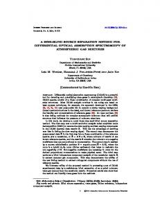
The source signal we use is a 2.4 sec (19200 samples for 8kHz sampling frequency) long audio recording of a musical instrument (violin)–see figure 2.
Figure 2: Source 1 - violin instrument It is important to understand how exactly an audio file is being recorded. Microphones are sensors in the soundfield, which record variations in the pressure of the air. Sound can be interpreted as air movement caused by vibrating objects. In acoustics, sound pressure is the potential energy component and particle velocity is the kinetic one. In order to measure the intensity of the sound (the product of the potential and kinetic energy), we need to relate to both pressure and velocity –see [5] and [3]. The medium we consider for the experiments is air at normal room temperature, as defined in equation 2.2. The pressure component is however included in the .wav file itself. Each sample represents a certain level of the air pressure at a point in time. As a result, we will consider Pa (Pascal) as being the unit on the y-axis for a sound file in all the simulations performed. Nevertheless, the relationship between pressure and voltage is linear (a microphone converts mechanical energy to electrical one), so we can use this proportionality later on when we compare the results of our experiments and we concentrate on analyzing the SNR level. The simulations for deriving the delay are based on the properties of the xcorr function defined in the Matlab library. xcorr(x,y) returns the cross-correlation sequence in a length 2*N-1 vector, where x and y are length N vectors (N > 1). If x and y are not the same length, the shorter vector is zero-padded to the length of the longer vector. The middle of the cross-correlation vector is considered to be in point N on the x-axis. Here, the autocorrelation function will return the highest peak. In a normal scenario, we expect the function to be symmetrical to the y-axis and give the maximum peak in point 0 (since cross-correlating a signal with itself should mean that there is a 0 delay between them). This is different in Matlab, where cross-correlation is not symmetrical to the y-axis anymore. It is simply a shifted by N version of the mathematically defined cross-correlation function. Therefore, we will always interpret point N as the equivalent of point 0. 6
We will test now if indeed, for a 0-delayed signal, autocorrelation will give a maximum peak in 0 (the N-corresponding value on the x-axis of the autocorrelation plot). In Matlab, we calculate xcorr(s1), where s1 was the original signal and plot it accordingly (see 3).
Figure 3: Autocorrelation source signal
Figure 4: Autocorrelation of delayed signal As we observe from figure 3, the maximum peak is at sample 19200, which is half of the total length of the autocorrelation (38400 samples). As the sampling frequency is 8kHz, this would correspond to a peak at 2.4 sec in a file of 4.8 sec (time = number of samples/sampling frequency). This was exactly what we expected to find: since the signal is not delayed, it would mean that the autocorrelation will be maximum in the middle of the file (2.4 sec delay corresponds to 0 sec delay as explained above). We will continue by applying a 25 msec delay to the original file (the equivalent of 200 samples) 7
and autocorrelating again the delayed signal (see figure 4). This figure has a peak at sample 19400, again half of the total length of 38800 samples, meaning that delayed s1 matches delayed s1. However, by comparing closely figures 3 and 4, we notice that they are shifted versions of each other, more exactly the second one is a shifted by 200 samples version of the first one (19400 - 19200 = 200). Since 200 is rather small in comparison with the total length of the two autocorrelation files, this is not immediately obvious and the only way to see it is by comparing the sample values where the highest peaks are found. We now consider a microphone mic1 placed where the source s1 is located (td1 = 0 msec delay) and another mic2 placed at 8.575m away (td2 = 25 msec delay). Crosscorrelating mic1 with mic2 should give us a peak at td1-td2 = -25msec (-200 samples) or at td2-td1 = 25msec (200 samples) if we cross-correlate mic2 with mic1 (see figure 5).
Figure 5: Delay estimation for source signal
We identify two peaks in both pictures: the first one is at 19200 and the second is at 19600. Since the entire length of the file is 38800 samples, the middle of it is at 19400. The first peak (19200 samples) is obtained by subtracting 200 samples from 19400 and the second peak (19600 samples) by adding 200 samples to 19400. So the two delays are of -200 samples and 200 samples respectively. In this particular case, we can calculate exactly the distance between microphone two and source (where microphone 1 is also located).
8
3.3
Random Signal Sources
For this simulation we consider 2 randomly generated signals s1 and s2 and two microphones mic1 and mic2. Microphone one records the sum of s1(t-td2) and s2(t-td1) and microphone two records s1(t-td1) and s2(t-td2). The scenario represents a special geometric case, where s1 is situated at the same distance from m1 as s2 is from m2, so they are symmetrically situated. We first try with large time delays: td1 = 200 samples and td2 = 112 samples. Crosscorrelation of mic1 and mic2 gives us the following picture:
Figure 6: Delay estimation for random source signals - large delays The two differences of delays are at 2000/2 + (112-200) = 1000 - 88 = 912 and 2000/2 + (200-112) = 1000 + 88 = 1088. So -88 samples and 88 samples are the two delay differences, which are accurately sketched on the plot. Now we apply the same scenario to a real-world situation: td1 = 30 samples (3.75 msec), equivalent to a distance of '1.28 m and td2 = 20 samples (2.5 msec), equivalent to a distance of '0.86 m. We still find accurate results in deriving the delay difference, which in this case is 10 samples (1.75 msec) – see figure 7.
3.4
Noise Considerations
In many situations, the quality of the recordings is affected by background noise. The more interference we have, the more difficult will be for our measurements to correctly identify the maximum cross-correlation values. In order to simulate a noisy environment, we add to the previous example two noise components, randomly generated and with a maximum amplitude of 20% of the source signals’ amplitude. Again, we test for two cases: big delays and small ones. In addition, we will analyze how different variations of noise values will influence our measurements. The noise components added to each microphone are independent of each other, so are separately generated and added. If we had dependent noise components, this would make quite difficult the analysis, since they would correlate with each other. However, in our scenario, the noise components will simplify each other (due to independence). Figure 9
Figure 7: Delay estimation for random source signals - small delays
8 shows the cases of different delay magnitudes, while figure 9 shows the small delay case with different noise ratios: 50% and 100% of the amplitude of the sound sources. We would like to analyze a larger variety of noise figures and see how SNR changes in accordance with the change in noise ratios. Therefore, we simulate 5 cases (noise ratio is 10%, 20%, 50%, 100% and 200%). The results are listed in the table below: Noise ratio 10% 20% 50% 100% 200%
Max A2signal 997.6 988.9 1003 938.2 1028
Max A2noise 189.1 179.3 236.2 310.8 549.4
SN Rmin 7.22dB 7.41dB 6.28dB 4.79dB 2.72dB A2
The minimum SNR was calculated with the following formula SN R[dB] = 10 log10 Asignal . 2 noise We observe that even for a small noise level, SNR is around 7 dB in value and if the noise increases strongly (200%), it decreases to 3 dB. Nevertheless, if we compare the two levels, the decrease of the SNR is much more slower than the increase of the noise level. Therefore, we conclude that different noisy environments with an acceptable noise ratio of up to 50% (and preferably around 20%) will not impose a major drawback.
3.5
Real Audio Signals Simulations
Until now we have considered only simple simulations, but we haven’t yet seen how mixtures of real audio files behave under similar circumstances. For this example we chose to work with .wav files from two instruments – a drum and a violin – which will be delayed and mixed together, noise also being added in a later scenario. Since the two instruments which were chosen are quite different, their plots also show this clearly (see figure 10). The drum file seems to be made of periodic peaks which decay slower or faster, while the violin file seems to display a more uniform behavior (decays are not that large and peaks 10
Figure 8: Delay estimation for noisy random source signals (different delays)
Figure 9: Delay estimation for noisy random source signals (different noise levels)
11
do not manifest high differences).
Figure 10: Audio Source Files We are going to build a similar setting as for the random signals: place the two microphones and the two sources symmetrical one to the other (would form an isosceles trapezoid). Let’s consider a distance of 2 m between the microphones and distances of 1.5 m and 1 m from each microphone to a source. This would mean '35 samples of delay (4.375 msec) and '23 samples of delay respectively (2.875 msec). The result of the simulation is found in figure 11. What we notice is that this time the simulations do not give us the exact delays any longer. We would normally expect two peaks at 38470/2 ± (35 − 23), so at sample 19247 and at sample 19223. However, we obtain peaks at slightly different values: 19250 and 19220. Microphone 1 is formed from the pair s1(t − 23) + s2(t − 35) and microphone 2 from the pair s1(t − 35) + s2(t − 23). As a result, the cross-correlation of the 2 microphones E[Mic1 Mic2]) contains 4 terms: E[s1(t − 23)]E[s1(t − 35)] + E[s1(t − 23)]E[s2(t − 23)] + E[s2(t − 35)]E[s1(t − 35)] + E[s2(t − 35)]E[s2(t − 23)]. All products s1 · s2 simplify (since they are 2 independent signals), so all we have left are terms E[s1(t−23)]E[s1(t−35)] and E[s2(t − 35)]E[s2(t − 23)]. Therefore, the plot should give us the difference in distances for source 1 at 23 - 35 = -12 samples and for source 2 at 35 - 23 = 12 samples. The first delay corresponds to s1, while the second to s2. However, the simulations give us peaks at 15 samples (19250) and -15 samples (19220). This means that the delay difference is calculated with a certain error(3 samples ' 0.13 meters). The error should be the same if we cross-correlate s2 with s1. 12
Figure 11: Cross-correlation of Audio Source Files
Figure 12: Cross-correlation of Audio Source Files 13
To prove that this assumption is correct, we plot the cross-correlation of microphone 2 and microphone 1 (see figure 12). We measure the highest peaks again and find out the values 19250 and 19220. We would expect this time a peak for source 1 at 12 samples and one for source 2 at -12 samples. What we actually measure is a peak at 15 (for s1) and one at -15 samples (for s2). So we just proved that our previous assumption holds.
3.6
Audio Files with Additional Noise and Distance Decay
We saw that dealing with real-world recordings can be a little tricky and we cannot always hope for perfect results. However, in real life, the situation is even worse: noise can make our measurements alter as well and we need to consider sound decay with distance (the α coefficient which we approximated to 1 until now). First of all, we consider the case where each microphone receives an additional noise component of 10% of amplitude of the signals (see figure 13). This doesn’t seem to
Figure 13: Noisy Audio Source Files change too much the situation, since we can still clearly identify the maximum peaks and we obtain the same sample points as we did when there was no additional noise at the microphones. However, as we increase the ratio of the noise, we obtain plots which are more difficult to measure and noise seems to become a real drawback from obtaining the real delays. Figure 14 describes 5 situations, where noise changes between 5% and 100%. In the random signal experiment, reaching value 100% still gave us good clear enough delay peaks, while here it is no longer possible to identify them. In conclusion, the algorithm will work efficiently only with lower than 50% noise ratios (20% gives us as
14
Figure 14: 5%, 10%, 20%, 50%, 100% Noisy Audio Source Files
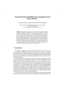
good estimates as a no-noise environment). Besides noise, each signal si decays by a coefficient αi , which is proportional with the inverse of distance. This can actually give us extra information regarding the true distance of the sources from the microphones. Let’s suppose a model in which sound decays with 0.95 in 1 meter and with 0.85 in 1.5 meters. We simulate and get the results in figure 15. It seems that the coefficient changes the situation (however, we do consider small distances, over which the coefficient is not much smaller than 1 anyway). The plots in figure 15 have a peak at 19250 corresponding to the delay difference of s2 and a peak at 19220 corresponding to the delay difference of s1. We observe that the peak at 19250 decreases from 79.84 to 64.09 Pa2 and the one at 19220 also changes from 79.98 to 64.98 Pa2 . Since pressure is proportional with voltage, so also with power and because power gets smaller with increasing distance (it is inversely proportional to the squared distance), we have the following relation: 0
00
00
P1 d1 2 t1 2 00 = 02 = 0 P1 d1 t12
(3.6.1)
From the plots, we derive the following relation of the distances between sources and microphones: 00 00 d2 2 d2 64.09 ' 0.8023 ⇒ = (3.6.2) 0 0 ' 0.8957 79.84 d22 d2
15
Figure 15: Audio Source Files with Distance Decay Coefficient
00
00
64.98 d d1 2 = ' 0.8124 ⇒ 10 ' 0.9013 0 79.98 d12 d1
(3.6.3) 00
One idea of interpreting equations 3.6.2 and 3.6.3 would be to compare values of 00 d2 0 d2
d1 0 d1
and
. We notice that the first one is larger, meaning that the new power of s1 is smaller than the new power of s2 – since d1 is the delay difference for first source. So the first source’s delay d1 should be increasing (distance increases), giving as a result a negative 0 0 00 00 difference of delays (∆delay = t1 − t1 < 0, where t1 > t1 ). This implies that the first source is closer to microphone 1. We know from the cross-correlation between microphones 1 and 2 (order is important in cross-correlation!) that we have a peak at a negative delay and one at a positive delay, which correspond to 2 delay differences, but we don’t know how large the distances themselves are. A further investigation of 3.6.2 and 3.6.3 might result in a new relationship that would allow us to identify the decaying factors. In this manner, we would be able to also gain some perspective on the actual distances to the sources and not just their difference.
3.7
Space Localization
In spite of the fact that we can only derive a relation of difference between the delays from the sources to the microphones, as long as this value is accurate, this can still be used for separating the sources (see algorithm proposed by Viste and Evangelista). In addition, 16
we can approximate on the actual place of the two sources by knowing the difference in distances from one source to each microphone. The hyperbola is the geometrical space of all points, from which the distance to two other fixed points is constant. Since the delay we measured doesn’t change, we can find the range of places where are sources could be by plotting the corresponding hyperbolas for each delay. First of all, we need to define the distance between the two microphones: dm = 2 meters ⇒ 2c = 2meters ⇒ c = 1 meter. We already know that both delay differences have the same absolute value, 2a = ∆d(meters)= 343m/sec · 0.0015sec (12 samples)= 0.5145 meters ⇒ a = 0.25725 meters. Since the semi-major axis √ a = 0.25725 m and we know c already, we can find out the semi-minor axis b as b = c2 − a2 ' 0.966 m. Using Matlab again, we plot the hyperbola associated with the respective values, while considering M1(-1,0) and M2(1,0) and the hyperbola centered at point (0,0) [2](see figure 16).
Figure 16: Source Localization
17
4
Conclusions and Future Developments
The simulations of this research paper were aimed at recreating various scenarios for BSS, on the basis of which, source localization and delay estimation were performed. We have seen cases in which delay estimation didn’t seem to cause any problem and cases where noise interferences led to a small error in determining the real values. In addition, we investigated a real case scenario of 2 microphones and 2 sources, for which we added time-decaying coefficients αi and derived the relationships in equations 3.6.1, 3.6.2, 3.6.3. A further analysis performed on real recordings (for which the actual α values can be calculated) might contribute to establishing a relationship between the rate of amplitude decay and the actual distances between sources and microphones, which is the goal of future investigations. Since noise levels can sometimes be a problem, another future project could be to build a filtering system which would at least reduce noise to an acceptable level. As we saw from our experiments, noise which has 20% of the signal amplitude doesn’t modify the performance of the cross-correlation between the mixtures, but for values greater than 50%, it doesn’t give results any longer. In order to improve our examples, it would be optimal to be able to come up with a solution to filter out the unwanted background noises.
References [1] Connexions. Correlation and covariance, 2005. [Online; accessed 12-May-2007]. [2] Matlab Central File Exchange. Create hyperbola. [Online; accessed 13-May-2007]. [3] Center for Computer Research in Music and Acoustics. Sound. [Online; accessed 13-May-2007]. [4] Gianpaolo Evangelista Harald Viste. Sound source separation: Preprocessing for hearing aids and structures audio coding. Proceedings of the COST G-6 Conference on Digital Audio Effects (DAFX-01), Limerick, Ireland, December 6-8, 2001. [5] E. Sengpiel. Microphone sensitivity conversion. [Online; accessed 13-May-2007]. [6] Wikipedia. Cocktail party effect — wikipedia, the free encyclopedia, 2006. [Online; accessed 8-May-2007]. [7] Wikipedia. Cross-correlation — wikipedia, the free encyclopedia, 2007. [Online; accessed 12-May-2007].
18