BLOCK PROCESSING WITH ITERATIVE

BLOCK PROCESSING WITH ITERATIVE CORRECTION FILTERS FOR TIME-INTERLEAVED ADCS Matthias Hotz and Christian Vogel FTW Telecommunications Research Center, Austria; E-mail: {hotz, c.vogel}@ieee.org fs /M ϕ = 2π MM−1

ABSTRACT This paper presents a systematic approach to block processing with iterative correction filters for time-interleaved analog-to-digital converters (TI-ADCs). TI-ADCs consist of several channels and can significantly increase the achievable sampling rate, but suffer from mismatches among the channels. Iterative digital correction filters are a general approach to mitigate the impact of mismatches in TIADCs. To reduce the requirements on the digital hardware, we introduce block processing for such filters. To this end, the transformation of a single-input single-output linear time-varying (LTV) finite impulse response filter into a multiple-input multiple-output LTV filter is described as a design equation and applied to two representative iterative correction structures from the literature. Finally, the beneficial properties and advantages of the transformation are highlighted.

u0 [m]

x ˆ0 [m]

ADC0 M −1−q fs /M ϕ = 2π M

x(t)

uq [m] ADCq

MIMO Correction Filter

x ˆq [m]

x ˆ[n]

0 fs /M ϕ = 2π M

uM −1 [m]

x ˆM −1 [m]

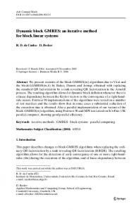
ADCM −1 Fig. 1. TI-ADC followed by a MIMO correction filter. The multiplexing of the output samples is visualized via a commutator [19].

Index Terms— time-varying filter, block processing, MIMO, Farrow structure, mismatch correction, time-interleaved ADC. 1. INTRODUCTION The significant demand for high-speed analog-to-digital converters (ADCs) gave rise to time-interleaved ADCs (TI-ADCs) [1]. TIADCs comprise M parallel channel ADCs operating at the rate fs /M , which are time-interleaved to yield samples of the input signal at the rate fs . Hence, compared to a single channel ADC, the output rate can be increased by a factor of M , but mismatches among the channels and clock skew can significantly degrade the performance [2]. Especially for medium and high-resolution TIADCs, the problem of impaired signals due to mismatches cannot be solved by analog design, but requires digital postprocessing [1]. Ideally, these postprocessing filters have a low implementation complexity as well as a low design complexity. The implementation complexity is the computational effort to operate the filter, e.g., the number of taps and the associated numbers of multiplications and additions, and the design complexity is the computational effort to compute the coeffcients with respect to the mismatches. The best trade-off between the implementation and design complexity depends on the application of the TI-ADC. In many cases, for example, where the correction filter is part of a blind identication and correction procedure, the design complexity outweighs the implementation complexity [3]. It is also desirable to have multiple-input multiple-output (MIMO) polyphase correction filters, which accept the direct output of the channel ADCs as a block of input samples The research leading to these results has received funding from the FFG Competence Headquarter program under the project number 835187. The Austrian Competence Center FTW Forschungszentrum Telekommunikation Wien GmbH is funded within the program COMET - Competence Centers for Excellent Technologies by BMVIT, BMWFJ, and the City of Vienna. The COMET program is managed by the FFG.

and work at an M -times lower rate fs /M as illustrated in Fig. 1, as they mitigate the speed requirements on the hardware and enable the use of more power and area efficient multipliers as shown in [4]. 2. CONTRIBUTIONS AND RELATION TO PRIOR WORK Many methods to correct mismatches have been proposed [5–18]. The correction methods either exhibit a high design complexity for changing mismatches [17, 18], do not utilize the advantages of a MIMO polyphase implementation by performing the correction on the full rate signal [5–7], or suffer from both [6, 7]. For particular mismatches such as time offsets, customized MIMO correction filters have been presented [14–16], which exploit the advantages of polyphase filtering and can adapt the coefficients with rather low complexity. A general concept for mismatch correction with low design complexity are iterative correction structures [8–13]. However, they have been established as single-input single-output (SISO) systems and, thus, lack the advantages of a MIMO polyphase implementation. In this paper, we introduce a systematic approach to obtain a MIMO polyphase implementation of iterative correction filters. To this end, a design equation for the structure of a MIMO LTV finite impulse response (FIR) filter is introduced, which utilizes the concepts in [20] to obtain a generalization of the design equation for block processing with linear time-invariant (LTI) FIR filters in [21] that maintains the same simplicity. The design equation is utilized to exemplify the transformation of SISO iterative correction filters to MIMO iterative correction filters by means of two representative structures, i.e., an iterative correction filter based on the Richardson iteration [13] and a correction filter for the reconstruction of nonuniform samples, the differentiator-multiplier cascade [8]. Therewith, the entire class of iterative correction filters [8–13] can utilize the advantages of a MIMO polyphase implementation as well.

λn

λn−1 z

−1

⇔

z

x[n]

v0 [n]

 yM

Hn (z)

−1

Fig. 2. Interchange of a time-varying multiplier λn , where n denotes the time dependence, and a delay element z −1 , which delays the signal by one sample [20].

3. DESIGN EQUATION FOR A MIMO LTV FILTER

y0 [m]

z −1

z v1 [n]

z

y[n]

x M

−1

This section establishes a design equation for a MIMO LTV filter that corresponds to a given SISO LTV filter by using the concepts presented in [20]. In the subsequent section, this design equation is utilized to attain block processing with iterative correction filters.

Hn−1 (z)

 yM

.. .

.. .

Hn−M +1 (z)

y1 [m]

x M .. .

z

vM −1 [n]  yM −1 [m] x yM M

Fig. 3. SISO LTV filter in multirate representation (cf. [19]). 3.1. SISO LTV Filter and Notation The output signal y[n] of a SISO LTV filter can be described by the convolution of the input signal x[n] with the time-varying impulse response hn [k], i.e., y[n] =

∞ X

FIR filters, the derivation may be pursued similarly, but the rule for interchanging time-varying multipliers and delay elements in Fig. 2 must be respected. Given this assumption, the M -fold polyphase decomposition of Hn (z) in (1) is given by [20]

hn [k]x[n − k] .

k=−∞

Hn (z) =

Since the conventional z-transform is not defined for a time-varying filter, it is defined here as the z-transform of the filter “frozen” at time instant n [20], i.e., Hn (z) =

∞ X

z

hn [k] .

It should be pointed out that delay elements and time-varying multipliers may not be interchanged without further consideration as in the time-invariant case, but the time dependency needs to be taken into account as well [20], cf. Fig. 2. In order to keep the underlying structure transparent in the z-domain, a refined notation is introduced. It is defined that the order of terms in equations in the z-domain corresponds to the structure of the underlying filter, i.e., a delay preceding a time-varying multiplier or LTV filter is written to its left, whereas a delay following it is written to its right. This implies that delay elements, LTV filters and time-varying multipliers do not commute under multiplication in the z-domain, but the rule in Fig. 2 must be respected. Furthermore, this concept of notation is extended to the z-transform of filters, i.e., FIR filters with the delay chain at the input (direct form) are denoted by writing the z to the left, as in (1), whereas FIR filters with the delay chain at the output (transposed form) are denoted by writing the z to the right [20]. 3.2. Derivation of the Design Equation A linear M -periodically time-varying filter may be represented as a time-invariant maximally decimated M -channel filter bank by processing M subsequent samples in parallel using the corresponding impulse responses and time-interleaving the results using decimators and expanders [19]. The same concept may as well be applied to a SISO LTV filter as depicted in Fig. 3, where, however, the resulting structure remains time-varying. Therein, the filters are followed by a decimator and a polyphase decomposition may be applied [19]. In order to keep the derivation as simple as possible, the interchange of time-varying multipliers and delay elements is avoided by assuming Hn (z) to be a direct form LTV FIR filter. For transposed form LTV

(2)

where the polyphase components are

(1)

k=−∞

˜ n(l) (z M ) z −l H

l=0

∞ X

˜ n(l) (z M ) = H −k

M −1 X

z −M k hn [M k + l] .

k=−∞

The output of the filter Hn−q (z) in channel q is identified as Vq (z) = X(z)z −q Hn−q (z) where q = 0, . . . , M − 1, cf. Fig. 3. The application of (2) yields Vq (z) =

M −1 X

M ˜ X(z)z −(q+l) H n−q (z ) (l)

(3)

l=0

where z −q and z −l were combined as both precede the filter ˜ (l) (z M ). In order to move the M -fold decimator in front of the H n−q

(l)

M 1 ˜ filter H n−q (z ), it is applied to Vq (z). Decimation is described in the z-domain by [19]

h i Yq (z) = Vq (z)

= ↓M

M −1 1 X r Vq (z 1/M WM ) M r=0

(4)

where WM is the M th root of unity, i.e., WM = e−2π/M . However, using (3) in (4) is not straightforward, as (4) is only capable of describing the implications in the z-domain and obscures the impact on the time-domain. Besides retaining only every M th sample and discarding the ones in between, which is well described by (4), the decimator further changes the time index from n before the decimator to m after the decimator, where one time step in m corresponds to M time steps in n, cf. Fig. 3. Taking this into account, the M -fold ˜ n(l) (z M ) leads to the polyphase components decimation of H (l)

HM m (z) =

∞ X

z −k hM m [k] (l)

(5)

k=−∞ 1 Note

that this corresponds to the Noble identity 1 [19] for LTV filters.

u0 [m]

MIMO Hn (z)

u1 [m]

MIMO Hn (z)

MIMO Hn (z)

x ˆ0 [m] x ˆ1 [m]

Fig. 4. 2-channel MIMO iterative correction filter based on the Richardson iteration. The 2-channel MIMO LTV filters are depicted in Fig. 5. x0 [m]

y0 [m]

(0)

H2m (z)

u[n]

x ˆ[n] Hn (z)

Hn (z)

Hn (z)

(1)

z −1

H2m−1 (z)

x1 [m]

y1 [m]

(0)

Fig. 6. Iterative correction filter based on the Richardson iteration.

H2m−1 (z) (1)

H2m (z) Fig. 5. 2-channel MIMO LTV filter associated with a direct form SISO LTV FIR filter Hn (z). The subfilters in the MIMO LTV filter are direct form FIR filters. with the corresponding impulse responses (l) hM m [k] = hn [M k + l]

n = Mm

where the change in the time index (n → M m) and extraction of every M th sample (z M → z) is respected. Considering these particularities, (3) may be used in (4), and in conjunction with (5) this results in Yq (z) =

M −1h X l=0

X(z)z −(q+l)

i

(l)

↓M

HM m−q (z)

(6)

(l)

where it was recognized that the input to the filters HM m−q (z) are time-shifted and decimated versions of the input signal. For a MIMO LTV filter, the input x[n] is provided in blocks of M samples, thus the channel input signals are identified as xr [m] = x[M m − r] with the corresponding z-transform h i Xr (z) = X(z)z −r

polyphase matrix in [20] and the generalization of the design equation for LTI filters in [21] to time-varying filters. It should be pointed out that the delay chain at the output in Fig. 3 is acausal and, therefore, not realizable. This stems from the dependence of the output block on the input block, thus a delay of z −M +1 is mandatory in a practical system. The MIMO LTV filter described by (7) is shown in Fig. 5 for M = 2. Note that the design equation (7) can be readily applied to correction structures based on adaptive direct form FIR filters, e.g., [5], and to linear M -periodically time-varying direct form SISO FIR filters, e.g., explicitly designed correction filters [6, 7]. 4. ITERATIVE CORRECTION FILTERS Iterative correction filters comprise a cascade of correction stages, where the error caused by the mismatches is reduced in every stage. Some of these correction filters are based on iterative methods known from computational mathematics, e.g., the Richardson iteration is utilized in [11, 13] and the Gauss-Seidel iteration is applied in [12], whereas others are derived explicitly, e.g., [8–10]. Using the design equation presented in Section 3, block processing with such structures may be directly accomplished. In favor of a compact discussion, this procedure is exemplified by means of two representative iterative correction filters. Based on this background, the extension to other iterative correction filters is rather straightforward.

↓M

where r = 0, . . . , M − 1. In order to map the channel inputs to the time-shifted and decimated input signals in (6), the delay z −(q+l) is considered, which is between z −2(M −1) and z 0 due to the range of q and l. A comparison of [X(z)z −(q+l) ]↓M to the definition of Xr (z) reveals that it equals Xq+l (z) if q + l ≤ M − 1 and Xq+l−M (z)z −1 if q + l > M − 1. Consequently, (6) can be expressed in terms of the channel input signals Xr (z) as Yq (z) =

M −1 X

Xhq+liM (z)z −b(q+l)/M c HM m−q (z) (l)

(7)

l=0

where b·c denotes the floor function and hkiM denotes the modulo operation, i.e., hkiM = k mod M . Eq. (7) specifies the output of channel q, i.e., Yq (z), in terms of the channel input signals Xr (z) and, therefore, can be regarded as a design equation for the structure of the MIMO LTV filter associated with the corresponding direct form SISO LTV FIR filter. Indeed, (7) is a reformulation of the

4.1. Richardson Iteration The SISO iterative correction filter presented in [13] is based on the Richardson iteration without relaxation and exhibits the fundamental structure depicted in Fig. 6, in which Hn (z) is a SISO LTV filter. If Hn (z) is a direct form FIR filter, the design equation (7) is directly applicable and provides the structure of the corresponding MIMO LTV filter. Therewith, the stages only need to be connected accordingly to obtain the MIMO iterative correction filter as illustrated in Fig. 4 for M = 2. If the filter Hn (z) delays the signal, corresponding delays need to be inserted into the SISO iterative correction filter as discussed in [13]. When this filter is transformed to a MIMO iterative correction filter, these delays must be implemented with block processing in mind. Assuming the signal should be delayed by D samples, then it suffices to delay all channel signals by D/M samples if D is a multiple of M , i.e., hDiM ≡ 0. However, if hDiM 6= 0, the channels need to be cross-connected to realize the delay, i.e., to de-

x0 [m] λn

u[n]

λn

−Hd (z)

x ˆ[n]

−Hd (z)

(1)

B0 (z)

λ2n

Stage 1

y0 [m]

(0)

B0 (z) λ2m

(0)

B1 (z)

− 12 Hd2 (z) Stage 2

(1)

B1 (z) Fig. 7. SISO DMC with 2 stages, in which Hd (z) is an ideal discrete-time differentiator and λn is the time-varying sampling time error in fractions of the sampling period.

(0)

B2 (z) z −1

Table 1. Polynomial Filters of the DMC Stages B0 (z)

B1 (z)

B2 (z)

Stage 1

0

−Hd (z)

0

Stage 2

0

−Hd (z)

−Hd2 (z)/2

λ2m

(1)

B2 (z) (1)

B2 (z) (0)

B2 (z) (1)

B1 (z)

λ2m−1

(0)

B1 (z)

lay the signal in channel q by D samples involves delaying it by b(q + D)/M c samples and connecting it to the channel hq + DiM of the subsequent structure.

(1)

B0 (z) x1 [m]

The differentiator-multiplier cascade (DMC) introduced in [8] is an iterative correction filter for timing mismatch correction based on a Taylor series expansion. A DMC with two stages is illustrated in Fig. 7, which realizes a Richardson iteration with reconstruction filters Hn (z) of increasing complexity. The structure of the stages can be identified as Farrow filters [22], which are linear FIR filters with a free parameter λn and utilized in various correction filters [8, 10–12]. The variation of the impulse response coefficients hn [k] with respect to λn is approximated with polynomials of degree P , i.e., P X

bp [k]λpn .

(8)

p=0

Therein, the subscript n denotes the dependence on the time index n and bp [k] are the coefficients of the polynomial for the coefficient hn [k]. In case of the DMC, the stages are Farrow filters with P = 2 and the polynomial filters given in Table 1. By applying (5), the polyphase components after decimation are given by (l)

HM m (z) =

P X

Bp(l) (z)λpM m

where the polyphase components are Bp(l) (z) =

y1 [m]

z −k b(l) p [k]

k=−∞ (l)

Fig. 8. 2-channel MIMO Farrow filter with P = 2.

5. DISCUSSION The MIMO filters obtained with the proposed approach comprise exactly M times the multipliers and adders of the corresponding SISO filters. Therefore, the number of arithmetic operations per unit time remains constant under the transformation, which implies that no computational overhead is introduced. Due to the transformation, the system rate of the correction filter is reduced by a factor of M , which mitigates the speed requirements on the hardware and enables the use of more power and area efficient multipliers as shown in [4]. Furthermore, the individual subfilters in the MIMO filter described by (7) comprise only 1/M th of the corresponding SISO LTV FIR filter coefficients and, as the transformation places at maximum M − 1 adders between the subfilters and the channel outputs, the critical path [21] is reduced as well if the order of the direct form SISO LTV FIR filter is at least M .

(9)

p=0

∞ X

(0)

B0 (z)

4.2. Differentiator-Multiplier Cascade

hn [k] =

λ2m−1

with the corresponding impulse responses bp [k] = bp [M k + l]. Using (9) in the design equation (7) yields the description of an M channel MIMO Farrow filter. The resulting structure is illustrated in Fig. 8 for M = 2 and P = 2. As the stages of the DMC are connected according to Fig. 6, the two stages of the considered 2channel MIMO DMC are connected as in Fig. 4, where the filters in the stages are 2-channel MIMO Farrow filters as shown in Fig. 8.

6. CONCLUSION In this paper, a systematic approach to block processing with iterative correction filters for TI-ADCs was presented. To this end, a design equation for a MIMO LTV filter was introduced, which permits block processing with direct form SISO LTV FIR filters for an arbitrary block length M . Using this design equation, block processing with iterative correction filters was introduced via the discussion of two representative structures, where the extension to other iterative correction filters is rather straightforward. Therewith, the class of iterative correction filters does not only exhibit a low design complexity, but can also take advantage of the benefits of a MIMO polyphase implementation.

7. REFERENCES [1] C. Vogel and H. Johansson, “Time-interleaved analog-todigital converters: Status and future directions,” in Proc. IEEE Int. Symp. Circuits and Systems (ISCAS 2006), May 2006, pp. 3386–3389. [2] C. Vogel, “The impact of combined channel mismatch effects in time-interleaved ADCs,” IEEE Trans. Instrumentation and Measurement, vol. 54, no. 1, pp. 415–427, Feb. 2005. [3] C. Vogel, M. Hotz, S. Saleem, K. Hausmair, and M. Soudan, “A review on low-complexity structures and algorithms for the correction of mismatch errors in time-interleaved ADCs,” Proc. IEEE Int. Northeast Workshop Circuits and Systems (NEWCAS) Conf., Jun. 2012. [4] M. Mottaghi-Dastjerdi, A. Afzali-Kusha, and M. Pedram, “BZ-FAD: A low-power low-area multiplier based on shiftand-add architecture,” IEEE Trans. VLSI Syst., vol. 17, no. 2, pp. 302–306, 2009. [5] S. Saleem and C. Vogel, “Adaptive compensation of frequency response mismatches in high-resolution timeinterleaved ADCs using a low-resolution ADC and a timevarying filter,” in Proc. IEEE Int. Symp. Circuits and Systems (ISCAS 2010), Jun. 2010, pp. 561–564. [6] H. Johansson and P. L¨owenborg, “Reconstruction of nonuniformly sampled bandlimited signals by means of time-varying discrete-time FIR filters,” EURASIP J. Applied Signal Processing, Jan. 2006. [7] H. Johansson and P. L¨owenborg, “A least-squares filter design technique for the compensation of frequency response mismatch errors in time-interleaved A/D converters,” IEEE Trans. Circuits and Systems II: Express Briefs, vol. 55, no. 11, pp. 1154–1158, Nov. 2008. [8] S. Tertinek and C. Vogel, “Reconstruction of nonuniformly sampled bandlimited signals using a differentiator–multiplier cascade,” IEEE Trans. Circuits and Systems I: Regular Papers, vol. 55, no. 8, pp. 2273–2286, Sep. 2008. [9] C. Vogel and S. Mendel, “A flexible and scalable structure to compensate frequency response mismatches in timeinterleaved ADCs,” IEEE Trans. Circuits and Systems I: Regular Papers, vol. 56, no. 11, pp. 2463–2475, Nov. 2009. [10] H. Johansson, “A polynomial-based time-varying filter structure for the compensation of frequency-response mismatch errors in time-interleaved ADCs,” IEEE J. Selected Topics in Signal Processing, vol. 3, no. 3, pp. 384 –396, Jun. 2009.

[11] K. M. Tsui and S. C. Chan, “A versatile iterative framework for the reconstruction of bandlimited signals from their nonuniform samples,” J. Signal Processing Systems, vol. 62, no. 3, pp. 459–468, Mar. 2011. [12] K. M. Tsui and S. C. Chan, “New iterative framework for frequency response mismatch correction in time-interleaved ADCs: Design and performance analysis,” IEEE Trans. Instrumentation and Measurement, vol. 60, no. 12, pp. 3792–3805, Dec. 2011. [13] M. Soudan and C. Vogel, “Correction structures for linear weakly time-varying systems,” IEEE Trans. Circuits and Systems I: Regular Papers, vol. 59, no. 9, pp. 2075–2084, Sep. 2012. [14] H˚akan Johansson and Per Lowenborg, “Reconstruction of nonuniformly sampled bandlimited signals by means of digital fractional delay filters,” IEEE Tran. Signal Processing, vol. 50, no. 11, pp. 2757–2767, 2002. [15] P. Satarzadeh, B.C. Levy, and P.J. Hurst, “A parametric polyphase domain approach to blind calibration of timing mismatches for M-channel time-interleaved ADCs,” in Proceedings of 2010 IEEE International Symposium on Circuits and Systems (ISCAS), 2010, pp. 4053–4056. [16] S. Huang and B.C. Levy, “Blind calibration of timing offsets for four-channel time-interleaved ADCs,” IEEE Trans. Circuits and Systems I: Regular Papers, vol. 54, no. 4, pp. 863–876, 2007. [17] R.S. Prendergast, B.C. Levy, and P.J. Hurst, “Reconstruction of band-limited periodic nonuniformly sampled signals through multirate filter banks,” IEEE Trans. Circuits and Systems I: Regular Papers, vol. 51, no. 8, pp. 1612–1622, 2004. [18] Munkyo Seo, Mark J W Rodwell, and U. Madhow, “Comprehensive digital correction of mismatch errors for a 400Msamples/s 80-dB SFDR time-interleaved analog-to-digital converter,” IEEE Trans. Microwave Theory Tech., vol. 53, no. 3, pp. 1072–1082, 2005. [19] P. P. Vaidyanathan, Multirate Systems and Filter Banks, Prentice Hall, Inc., Upper Saddle River, NJ, USA, 1993. [20] See-May Phoong and P. P. Vaidyanathan, “Time-varying filters and filter banks: Some basic principles,” IEEE Trans. Signal Processing, vol. 44, no. 12, pp. 2971–2987, Dec. 1996. [21] Keshab K. Parhi, VLSI Digital Signal Processing Systems: Design and Implementation, John Wiley & Sons, Inc., 1999. [22] C. W. Farrow, “A continuously variable digital delay element,” in Proc. IEEE Int. Symp. Circuits and Systems (ISCAS 1988), Jun. 1988, vol. 3, pp. 2641–2645.