i
Boosting Lazy Abstraction for SystemC with Partial Order Reduction Alessandro Cimatti, Iman Narasamdya, and Marco Roveri FBK-Irst {cimatti,narasamdya,roveri}@fbk.eu Abstract. The SystemC language is a de-facto standard for the description of systems on chip. A recent approach to the formal verification of SystemC designs, called ESST, combines Explicit state techniques to deal with the SystemC Scheduler, with Symbolic techniques, based on lazy abstraction, to deal with the Threads. Despite its relative effectiveness, this approach suffers from the potential explosion of thread interleavings. In this paper, we propose the adoption of partial order techniques to alleviate the problem. We extend the ESST with two complementary PO techniques (persistent set, and sleep set), and we prove the soundness of the approach in the case of safety properties. The extension is only seemingly trivial: the PO reduction, applied to the scheduler, must be proved not to interfere with the lazy abstraction of the threads. We implemented the techniques within the software model checker S Y CMC, and we carried out an experimental evaluation on benchmarks taken from the SystemC distribution and from the literature. The results showed a significant improvement, both in the number of visited abstract states, and in run times.
1
Introduction
SystemC has widely been used for the design of executable models of systems on chip. It allows for high-speed simulation before synthesizing the RTL hardware description. Verification of SystemC designs is an important issue since errors identified in such models can reveal errors in the specification and prevent error propagation down to the hardware. Despite its importance, formal verification of SystemC is still at a preliminary stage. Indeed, a SystemC design is a very complex entity, that can be thought of as multi-threaded software, where scheduling is cooperative and carried out according to a specific set of rules [21], and the execution of threads is mutually exclusive. A promising technique, called ESST [7], has recently been proposed for the verification of SystemC designs. ESST combines Explicit state techniques to deal with the SystemC Scheduler, with Symbolic techniques, based on lazy abstraction [2], to deal with the Threads. Despite its relative effectiveness, the ESST techniques suffers from two main inefficiencies. First, it has to perform several expensive predicate abstractions during the exploration of threads. Second, due to keeping track of the scheduler states explicitly, it has to explore a large number of thread interleavings, but many of which are redundant. These inefficiencies degrades the run time performance and can cause out of memory due to state explosion. Partial-order reduction (POR) [11, 19, 23] has been proposed as a model checking technique for combating the state explosion by exploring only representative subset of all possible schedules. POR exploits the commutativity of concurrent transitions
that results in the same state when they are executed in different orders. It has successfully been applied in explicit-state software model checkers like SPIN [13] and V ERI S OFT [10], and also in symbolic model checking as shown in [15, 24, 1]. In this paper, we investigate the application of POR to the ESST technique. We considered two complementary POR techniques: the persistent set and the sleep set [11]. These two sets are used by the ESST algorithm in deciding which threads to expand, while the symbolic search remains unchanged. We remark that the application of POR in ESST algorithm is only seemingly trivial since it must be proved not to interfere with the lazy abstraction used for the search within the threads. We proved the soundness of the approach in the case of verification of safety properties. We implemented these POR techniques within the ESST algorithm as implemented in the S Y CMC software model checker which is part of the tool chain described in [7]. The tool chain includes a SystemC front-end derived from P INAPA [17]. The front-end first translates a SystemC design into a threaded C program. In such a C program each thread in the SystemC design is represented as a C function. We carried out a thorough experimental evaluation on benchmarks taken from the SystemC distribution and from the literature. The results showed a significant improvement w.r.t. the ones reported in [7], both in the number of visited abstract states, and in run times. This paper is structured as follows. In Section 2 we briefly introduce SystemC and we briefly describe the ESST algorithm. In Section 3 we show by means of an example the possible state explosion problem that may arise. In Section 4 we show how to lift POR techniques to the ESST algorithm. In Section 5 we revise the related work. Finally, in Section 7 we draw some conclusions and we outline future work.
2 2.1
Background The SystemC language
SystemC is a C++ library that consists of (1) a core language that allows one to model a System-on-Chip (SoC) by specifying its components and architecture, and (2) a simulation kernel (or scheduler) that schedules and runs processes (or threads) of components. SoC components are modeled as SystemC modules that communicate through channels (that are bound to the ports specified in the modules). The SystemC library provides primitive channels such as signal, mutex, semaphore and queue. A module consists of one or more threads that describe the parallel behavior of the SoC design. SystemC provides general-purpose events as a synchronization mechanism between threads. For example, a thread can suspend itself by waiting for an event or by waiting for some specified time. A thread can perform immediate notification of an event or delayed notification. The SystemC scheduler is a cooperative non-preempting scheduler that runs at most one thread at a time. During a simulation, the status of a thread changes from sleeping, to runnable, and to running. A running thread will only give control back to the scheduler by suspending itself. The scheduler runs all runnable threads, one at a time, in a
single delta cycle, while postponing the channel updates made by the threads. When there are no more runnable threads, the scheduler materializes the channel updates, and wakes up all sleeping threads that are sensitive to the updated channels. If, after this step, there are some runnable threads, then the scheduler moves to the next delta cycle. Otherwise, it accelerates the simulation time to the nearest time point where a sleeping thread or an event can be woken up. The scheduler quits when there are no more runnable threads after time acceleration. An example of SystemC design is shown in Figure 1. The example is adapted from and a simplified version of the pipeline example taken from the SystemC distribution [18]. This example consists of three modules, numgen, stage1, and stage2. In the sc main function we create an instance for each module, and we connect them such that the instances of numgen and stage1 are connected by the signal gen to s1 and the instances of stage1 and stage2 are connected by the signal s1 to s2. The thread generate of numgen reads an integer value from the environment and sends it to stage1 through the signal gen to s1. The thread pass of stage1 simply reads the value from the signal gen to s1 and sends it to stage2 through the signal s1 to s2. The thread check of stage2 reads the value from s1 to s2 and asserts that the read value equals 0. All threads are made sensitive to the positive edge of the clock clk. That is, they become runnable when the value of the clock, which is modeled as a boolean signal, changes from 0 to 1. The function dont initialize makes the most-recently declared thread sleep initially. The clock cycle is controlled by the loop in the sc main function. The function sc start runs a simulation until there are no more runnable threads. The property that we want to check is that the value read by numgen from the environment reaches stage2 in three clock cycle. 2.2
The Explicit Scheduler + Symbolic Threads (ESST) approach
The ESST technique [7] is a counter-example guided abstraction refinement [8] based technique that combines explicit-state technique with lazy predicate abstraction [2]. In the same way as the classical lazy abstraction, the data path of the threads is analyzed by means of predicate abstraction, while the flow of control of each thread and the state of the scheduler are analyzed with explicit-state techniques. We assume that the SystemC design has been translated into a threaded C program [7] in which each SystemC thread is represented by a C function. Each function corresponding to a thread is represented by a control-flow automaton (CFA), which is a pair (L, G), where L is the set of control locations and G ⊆ L × Ops× is the set of edges such that each edge is labelled by an operation from the set Ops of operations. Threads in a threaded C program communicate with each other by means of shared global variables, and use primitive functions and events as synchronization mechanism. For SystemC we have the following primitive functions: wait event(e) and wait time(t) to suspend the thread itself and, respectively, to wait for the notification of the event e and to wait for a time unit t; notify event(e) to notify the event e immediately, notify event at time(e,t) to notify event e with delayed time t, and cancel event(e) to cancel a delayed notification of event e.
1 2 3 4 5 6 7 8 9 10 11 12 13 14 15 16 17 18 19 20 21 22 23 24 25 26 27 28 29 30 31 32 33 34 35 36 37 38 39
SC MODULE( numgen ) { sc out o u t ; / / output port . sc in c l k ; / / input port f o r clock . / / Reads i n p u t from environment . void generate ( ) { int i = read input ( ) ; out . w r i t e ( i ) ; } SC CTOR( numgen ) { / / d e c l a r e ” generate ” as a method t h r e a d . SC METHOD( generate ) ; dont initialize (); / / make i t s e n s i t i v e t o p o s i t i v e c l o c k edge . s e n s i t i v e 0 such that there is a path γ0
γ1
γm−1
s0 → s1 → · · · → sm , where for all i = 0, . . . , m − 1, the set Pi is the persistent set in state si , the transition γi is in Pi , and the transition α in not in Pi (see Figure 3). First, the above path exists because of the successor-state condition and it must be finite because the set S of states is finite. The path cannot form a cycle, otherwise by the cycle condition the transition α will have been in the persistent set in one of the states that form the cycle. That is, by the above path, we delay the exploration of α as long as possible. Second, since the transition α is enabled in s0 and is independent in si of any transition in Pi for all i = 0, . . . , m − 1 (otherwise Pi is not a persistent set), then α remains enabled in sj for j = 1, . . . , m. Third, since m is the greatest number, we have α in the persistent set in the state α sm , and furthermore sm → s0e holds for an error state s0e . Thus, the path γm−1 γ0 α s0 → · · · → sm → s0e is the path from s0 leading to an error state s0e involving only transitions in the persistent sets of visited states. Case n = 2. Let s0 ∈ S be such that there is a path β0
β1 =α
s0 → s01 → se for some state s01 and an error state se . By the successor-state condition, the persistent set in s0 is non-empty. If the only persistent set in s0 is the singleton set {β0 }, β0
then the path s0 → s01 consists only of transition in the persistent set. By the case n = 1, it is guaranteed that there is a path from s01 leading to an error state s0e such that the path consists only of transitions in the persistent sets of visited states. Thus, there is a path from s0 leading to an error state s0e such that the path consists only of transistions in the persistent sets of visited states. Suppose that the transition β0 is not in the persistent set in s0 . Take the greatest m > 0 such that there is a path γ0
γ1
γm−1
s0 → s1 → · · · → sm , where for all i = 0, . . . , m − 1, the set Pi is the persistent set in state si , the transition γi is in Pi , and the transition β0 in not in Pi (see Figure 4). With the same reasoning as in the case of n = 1, the above path exists, and is finite and acyclic. That is, we delay the exploration of β0 as long as possible. Consider now the path γ0
γ1
γm−1
β0
s0 → s1 → · · · → sm → s0m+1 . We show that an error state is reachable from the state s0m+1 . First, since the transitions γ0 and β0 are independent in s0 , the transitions γ0 and β0 are enabled,
respectively, in the states s01 and s1 , and they commute in the state s02 . The transition γ0 is also independent of the transition α in s01 , otherwise P0 is not a persistent set in s0 . Thus, the transition α is enabled in s02 . Second, since the transitions γ1 and β0 are independent in s1 , the transitions γ1 and β0 are enabled, respectively, in the states s02 and s2 , and they commute in the state s03 . The transition γ1 is independent of the transition α in s02 , otherwise P1 is not a persistent set in s1 . Thus, the transition α is enabled in s03 . By repeatedly applying the above reasoning, it follows that the transition α is enabled in the state s0m+1 . If the singleton set {α} is the only persistent set in s0m+1 , then we are done. That is, the path γ0
γ1
γm−1
β0
α
s0 → s1 → · · · → sm → s0m+1 → s0e is the path from s0 leading to an error state s0e such that it consists only of transistions in the persistent sets of visited states. In the same way as in the case of n = 1, if the transition α is not in the persistent set in s0m+1 , then we can delay α as long as possible by taking the greatest k > 0 such that there is a path γm+1
γm
s0m+1 → s0m+2 → · · ·
γm+k−1
→
s0m+k+1 ,
where for all l = 1, . . . , k + 1, the set Pm+l is the persistent set in state s0m+l , the transition γm+l−1 is in Pm+l , and the transition α in not in Pm+l . Thus, the path γ0
γ1
γm−1
β0
s0 → s1 → · · · → sm → s0m+1 · · ·
γm+k−1
→
α
s0m+k+1 → s0e
is the path from s0 leading to an error state s0e such that it consists only of transitions in the persistent sets of visited states. Case n > 0. Let s0 ∈ S be such that there is a path β0
β1
s0 → s01 → · · ·
βn−1 =α
→
se
for some state s01 and an error state se . By the successor-state condition, the persistent set in s0 is non-empty. If the only persistent set in s0 is the singleton set {β0 }, β0
then the path s0 → s01 consists only of transition in the persistent set. By the case n = 1, it is guaranteed that there is a path from s01 leading to an error state s0e such that the path consists only of transitions in the persistent sets of visited states. Thus, there is a path from s0 leading to an error state s0e such that the path consists only of transistions in the persistent sets of visited states. Suppose that the transition β0 is not in the persistent set in s0 . Take the greatest m > 0 such that there is a path γ0
γ1
γm−1
s0 → s1 → · · · → sm , where for all i = 0, . . . , m − 1, the set Pi is the persistent set in state si , the transition γi is in Pi , and the transition β0 in not in Pi (see Figure 5). That is, we delay the exploration of β0 as long as possible.
Consider now the path γ0
γm−1
γ1
β0
s0 → s1 → · · · → sm → s0m+1 . With the same reasoning as in the case of n = 2, we have the transition β1 enabled in the state s0m+1 , and we can postpone the exploration of β1 as long as possible. When β1 gets explored, the transition β2 is enabled in the successor state. By repeatedly applying the same reasoning for transitions βk for k = 2, . . . , n − 1, the path formed in a similar way to that of the case of n = 2 is the path from s0 leading to an error state s0e such that the path consists only of transitions in the persistent sets of visited states. t u s0 γ0
α
s1
se
γ1
α
s2 α sm−1 γm−1 sm
α α s′e
Fig. 3. Case n = 1 of the proof of Theorem 4.4. s0
γ0 s1 γ1 β0 sm−1 β0 β0 γm
s′1 γ0 β1 = α s′2 se γ α ′ 1
β0
s2 γm−1 sm
β0
s3 α
s′m α γ ′ m−1
sm+1 α
s′m+2 α s′m+k γm+k−1
α
s′m+k+1 α s′e
Fig. 4. Case n = 2 of the proof of Theorem 4.4.
An important insight from the above proof is when the transition system is unsafe, then the state-space exploration with POR can visit more states than that of when the exploration is performed without POR. For example, in the case of n = 1 above, if the state s0 is in the set of initial states, then the state-space exploration without POR only needs to visit two states s0 and se to decide that the transition system is unsafe. However, when POR is applied to the state-space exploration, then as shown in the proof the exploration visits more than two states.
s0 γ0
β0
s1 γ1
β0
s2 β0 sm−1 γm−1 sm β0
γ1 s′3 β1
β0 s′m α γ m−1 ′
sm+1 β1
γ ′ 0
s2 β1
s′1 β1 γ0
γ1
γ0 γ1
α
βn−1 = α se
α
γm−1 γm−1α α
Fig. 5. Case n > 0 of the proof of Theorem 4.4.
The Sleep Set approach We consider also the sleep set POR technique. This technique exploits independencies of enabled transitions in the current state. For example, suppose that in some state s there are two enabled transitions α and β, and they are independent of each other. Suppose further that the search explores α first from s. Then, when the β
search explores β from s such that s → s0 for some state s0 , we associate with s0 a sleep set containing only α. From s0 the search only explores transitions that are not in the sleep set of s0 . That is, although the transition α is still enabled in s0 , it will not be explored. Both persistent set and sleep set techniques are orthogonal and complementary, and thus can be applied simultaneously. Note that the sleep set technique only removes transitions, and not states. Thus Theorem 4.4 still holds when the sleep set technique is applied. 4.2
Applying POR to ESST
Applying POR to the ESST algorithm is not trivial. First, the ESST algorithm analyzes the CFA’s of functions representing threads, while the program considered in the exposition of POR in the previous sub-section is represented by a transition system. One then needs to identify what constitute a transition in the CFA’s of a thread. Second, the construction of a valid dependence relation has to consider primitive functions that can update the status of threads and events. For example, transitions can perform immediate event notification that makes other threads runnable and cancel a delayed event notification. Third, the ESST algorithm is based on the construction of an ARF that describes the reachable abstract states of the threaded program, while the exposition of POR before is based on the analysis of reachable concrete states. One then needs to guarantee that the original ARF is safe iff. the reduced ARF, obtained by applying POR in the construction of ARF, is safe. That is, we have to ensure that the selective search performed during the construction of ARF does not remove all non-spurious paths that lead to error locations. In particular, the construction of reduced ARF has to check if the cycle condition is satisfied in its concretization. To integrate POR techniques into the ESST algorithm we first need to identify transitions in the threaded program. In the above description of POR the execution of a
transition is atomic. We introduce the notion of atomic block as the notion of transition in the threaded program. Intuitively an atomic block is a block of operations between calls to primitive functions that can suspend the thread. For simplicity, let us call such primitive functions wait functions. An atomic block of a thread is a rooted subgraph of the CFA satisfying the following conditions: (1) its unique entry is the entry of the CFA or the location that immediately follows a call to a wait function; (2) its exit is the exit of the CFA or the location that immediately follows a call to a wait function; and (3) there is no call to a wait function in any CFA path from the entry to an exit except the one that precedes the exit. Note that an atomic block has a unique entry, but can have multiple exits. We often identify an atomic block by its entry. For example, consider the thread code below: void thread_t() { while (...) { ... wait_event(e); l: ... } } The thread has two atomic blocks. One atomic block starts from the entry of the thread and ends at the label l and at the exit of the thread. The other atomic block starts from the label l and ends at the label l too and at the exit of the thread. In the sequel we will use the terms transition and atomic block interchangeably. We use static analysis techniques to compute a valid dependence relation. In particular, a pair (α, β) of atomic blocks are in a valid dependence relation if the following criteria are satisfied: 1. The atomic block α contains a write to a shared (or global) variable g, and the atomic block β contains a write or a read to g. 2. The atomic block α contains an immediate notification of an event e, and the atomic block β contains a wait for e. 3. The atomic block α contains a delayed notification of an event e, and the atomic block β contains a cancellation of a notification of e. Persistent sets are computed using a valid dependence relation. Let D be a valid dependence relation. Algorithm 1 computes persistent sets. The else-branch of the algorithm can be implemented as follows. If the atomic block α and the thread that owns α sleeps at the entry of β different form α, then we add β into P if there is a path from β to α. If the atomic block α is the same as β, then we add all atomic blocks that can immediately notify the event that α is waiting for. It is easy to see that the persistent set computed by Algorithm 1 satisfies the successor-state condition. Algorithm 1 is a variant of the stubborn set algorithm presented in [11], that is, we use a valid dependence relation as the interference relation described in [11]. We apply POR to the ESST algorithm by modifying the ARF node expansion rule E2, described in Section 2.2 in two steps. The first step amounts to computing
Algorithm 1 Persistent set. Input: a set TE of enabled atomic blocks. Output: a persistent set P . 1. Let TP := {α}, where α ∈ TE . 2. For each atomic block α ∈ TP : (a) If α ∈ TE (α is enabled): – Add into TP every atomic block β such that (α, β) ∈ D. (b) If α 6∈ TE (α is disabled): – Add into TP a set of atomic blocks whose executions guarantee α to become enabled. 3. Repeat step 2 until no more transition can be added into TP . 4. P := TP ∩ TE .
a persistent set from a set of scheduler states output by the function S CHED. The second step amounts to ensuring that the cycle condition is satisfied by the concretization of the constructed ARF. First, we assume that a valid dependence relation D has been produced by static analysis on the threaded program. Second, we introduce the function P ERSISTENT that computes a persistent set of a set of scheduler states. P ERSISTENT takes as inputs an ARF node and a set S of scheduler states, and outputs a subset S 0 of S. The input ARF node keeps track of the thread locations, which are used to identify atomic blocks, while the input scheduler states keep track of the status of the threads. From the ARF node and the set S, the function P ERSISTENT extracts the set TE of enabled atomic blocks. P ERSISTENT then computes a persistent set P from TE using Algorithm 1. Finally P ERSISTENT constructs back a subset S 0 of the input set S of scheduler states from the persistent set P . Let A = (hl1 , ϕ1 i, . . . , hln , ϕn i, ϕ, S) be an ARF node that is going to be expanded. We replace the rule E2 in the following way: instead of creating a new ART for each state S 0 ∈ S CHED(S), we create a new ART whose root is the node (hl1 , ϕ1 i, . . . , hln , ϕn i, ϕ, S 0 ) for each state S 0 ∈ P ERSISTENT(A, S CHED(S)) (rule E2’). To guarantee the preservation of safety properties, we have to check that the cycle condition is satisfied. Following [9] we check a stronger condition: at least one state along the cycle is fully expanded. In the ESST algorithm a potential cycle occurs if an ARF node is covered by one of its predecessors in the ARF. Let A = (hl1 , ϕ1 i, . . . , hln , ϕn i, ϕ, S) be an ARF node. We say that the scheduler state S is running if there is a running thread in S. Recall our assumption that there is at most one running thread in the scheduler state. We also say that the node A is running if its scheduler state S is. Note that during ARF expansion the input of S CHED is always a non-running scheduler state. A path in an ARF can be represented as a sequence A0 , . . . , Am of ARF nodes such that for all i, we have Ai+1 is a succcessor of Ai in the same ART or there is an ARF connector from Ai to Ai+1 . Given an ARF node A of ARF F , we denote by ARFPath(A, F ) the ARF path A0 , . . . , Am such that (1) A0 has neither a predecessor ARF node nor an incoming ARF connector, and (2) Am = A. Let Π be an ARF path, we denote by NonRunning(Π) the maximal subsequence of non-running node in Π.
Algorithm 2 ARF expansion algorithm for non-running node. Input: a non-running ARF node A that contains no error locations. 1. Let NonRunning(ARFPath(A, F )) be A0 , . . . , Am such that A = Am 2. If there exists i < m such that Ai covers A: (a) Let Am−1 = (hl10 , ϕ01 i, . . . , hln0 , ϕ0n i, ϕ0 , S 0 ). (b) If P ERSISTENT(Am−1 , S CHED(S 0 )) ⊂ S CHED(S 0 ): – For all S 00 ∈ S CHED(S 0 ) \ P ERSISTENT(Am−1 , S CHED(S 0 )): • Create a new ART with root node (hl10 , ϕ01 i, . . . , hln0 , ϕ0n i, ϕ0 , S 00 ). 3. If A is covered: Mark A as covered. 4. If A is not covered: Expand A by rule E2’.
Algorithm 2 shows how a non running ARF node A is expanded in the presence of POR. We assume that A contains no error locations. Essentially, the algorithm fully expands the immediate non-running predecessor node of A when a potential cycle is detected. Otherwise the node is expanded as usual. Our POR technique differs from that of in [9], which is implemented in SPIN [14]. The technique in [9] tries to select a persistent set that does not create a cycle, and if it does not succeed, then it fully expands the node. In the context of ESST such a technique is expensive. To detect a cycle one has to expand a node by a transition. As explained before, a transition or an atomic block in our case can span over multiple operations in CFA. Thus, a cycle detection often requires expensive computations of abstract strongest post condition. In addition to coverage check, in the above algorithm one can also check if the detected cycle is spurious or abstract. We only fully expand a node iff the detected cycle is not spurious. As cycles are rare, the benefit of POR can be defeated by the price of generating and solving the constraints that encode the cycle. In SystemC cycles can occur because there is a chain of wait and immediate notifications of events. For SystemC cycle detection can be optimized by only considering the sequence of non-running ARF node that belongs to the same delta-cycle. POR based on sleep set can also be applied to ESST. First, we extend the node of ARF to include a sleep set. That is, an ARF node is a tuple (hl1 , ϕ1 i, . . . , hln , ϕn i, ϕ, S, Z), where the sleep set Z is a set of atomic blocks. The sleep set is ignored during coverage check. Second, from the set of enabled atomic blocks and the sleep set of the current node, we compute a subset of enabled atomic blocks and a mapping from every atomic block in the former subset to a successor sleep set. Let D be a valid dependence relation, Algorithm 3 shows how to compute a reduced set of enabled transitions TR and a mapping MZ to successor sleep sets using D. The input of the algorithm is a set TE of enabled atomic blocks and the sleep set Z of the current node. Note that the set TE can be a persistent set obtained by Algorithm 1. Similar to the persistent set based technique, we introduce the function S LEEP that takes as inputs an ARF node A and a set of scheduler states S, and outputs a subset S 0 of S along with the above mapping MZ . From the ARF node and the scheduler states, S LEEP extracts the set TE of enabled atomic blocks and the current sleep set. S LEEP then computes a subset TR of TE of enabled atomic blocks and the mapping MZ using Algorithm 3. Finally S LEEP constructs back a subset S 0 of the input set S of scheduler states from the set TR of enabled atomic blocks.
Algorithm 3 Sleep set. Input: – a set TE of enabled atomic blocks. – a sleep set Z. Output: – a reduced set TR ⊆ TE of enabled atomic blocks. – a mapping MZ : TR → TE × TR . 1. TR := TE \ Z. 2. For all α ∈ TR : (a) For all β ∈ Z: – If (α, β) 6∈ D (α and β are independent): MZ [α] := MZ [α] ∪ {β}. (b) Z := Z ∪ {α}.
Let A = (hl1 , ϕ1 i, . . . , hln , ϕn i, ϕ, S, Z) be an ARF node that is going to be expanded. We replace the rule E2 in the following way: let (S 0 , MZ ) = S LEEP(A, S CHED(S)), create a new ART whose root is the node (hl1 , ϕ1 i, . . . , hln , ϕn i, ϕ, S 0 , MZ [l0 ]) for each S 0 ∈ S 0 such that l0 is the atomic block of the running thread in S 0 . One can easily combine persistent and sleep set by replacing (S 0 , MZ ) = S LEEP(A, S CHED(S)) above by (S 0 , MZ ) = S LEEP(A, P ERSISTENT(A, S CHED(S))). 4.3
Correctness of Reduction in ESST
The correctness of POR with respect to verifying program assertions of transition systems has been shown by Theorem 4.4. The correctness proof relies on the enabledness and commutativity of independent transitions. However, the proof is applied in concrete state space of the transition system, while the ESST algorithm works in abstract state space represented by an ARF. The following observation shows that two transition that are independent in the concrete state space may not commute in the abstract state space. For simplicity of presentation, we represent an abstract state by a formula representing a region. Let g1 , g2 be global variables, and p, q be predicates such that p ⇔ (g1 < g2 ) and q ⇔ (g1 = g2). Let α be the transition g1 := g1 - 1 and β be the transition g2 := g2 - 1. It is obvious that α and β are independent of each other. However, Figure 6 shows that the two transition do no commute when we start from an abstract state A1 such that A1 ⇔ p. The edges in the figure represent the computation of abstract strongest post condition of the corresponding abstract states and transitions. Even though two independent transitions do not commute in abstract state space, they still commute in the concrete state space overapproximated by the abstract state space, as shown by the lemma below. For a concrete state s and an abstract state A, we write s |= A iff A holds in s. L EMMA 4.5 Let α and β be transitions that are independent of each other such that for concreate states s1 , s2 , s3 and abstract state A we have s1 |= A, and both α(s1 , s2 ) and β(s2 , s3 ) holds. Let A0 be the abstract successor state of A by applying the abstract strongest post operator to A and β, and A00 be the abstract successor state of A0 by applying the abstract strongest post operator to A0 and α.
A1 (p) α A2 (p) β A3 (p ∨ q)
β A4 (p ∨ q) α A5 (p)
Fig. 6. Independent transitions do not commute in abstract state space.
Then, there are concrete states s4 and s5 such that: (1) β(s1 , s4 ) holds, (2) s4 |= A0 , (3) β(s4 , s5 ) holds, (4) s5 |= A00 , and (5) s3 = s5 . Proof. By the independence of α and β, we have β(s1 , s4 ) holds. By the abstract strongest post operator, we have s4 |= A0 . By the independence of α and β, we have β(s4 , s5 ) holds. By the abstract strongest post operator and the fact that s4 |= A0 , we have s5 |= A00 . Finally by the independence of α and β, we have s3 = s5 . t u The above lemma shows that POR can be applied in abstract state space. We now can prove the correctness of the reduction in the ESST technique, as stated by the following theorem: T HEOREM 4.6 Let ARF F1 be obtained by node expansion without POR and ARF F2 be obtained with POR. F1 is safe iff F2 is safe. Proof. If F1 is safe, then F2 is obviously safe because POR only reduces the number of explored transitions and thus removes abstract states. For the other direction, it follows from Theorem 4.4 in conjuction with Lemma 4.5 that if there is a non-spurious path to an error state in F1 , then there is also a non-spurious path to an error state in F2 . t u
5
Related Work
In [3] is discussed an approach aiming at the generation of a SystemC scheduler from a SystemC design that at run time will use race analysis information to speed up the simulation by reducing the number of possible interleavings. The race condition itself is formulated as a guarded independence relation. The independence relation used in [3] is more precise than the one defined in this paper. In our work two transitions are independent if they are independent in any state. While in [3] two transitions are independent in some state if the guard associated with the pair of transitions is satisfied by the state. The guards of two transitions are computed using model checking techniques. The soundness of the synthesized scheduler relies on the assumption that the SystemC threads cannot enable each other during the evaluation phase. Therefore, immediate event notifications are not allowed. Our work does not have such an assumption. Moreover, unlike our work, the search in [3] is stateless and it is bounded on the number of simulation steps: cycle condition cannot be detected, and thus this approach cannot be used to verify program assertions.
Dynamic POR techniques for scalable testing of SystemC designs are described in [16, 12]. Unlike other works on dynamic POR that collect and analyze run time information to determine dependency of transitions, the work in [16] uses information obtained by static analysis to construct persistent set. For SystemC the criteria that they use to determine dependency of transitions are similar to the criteria we used in this paper. However, similarly to [3], the simulation is bounded and stateless, and thus cannot be used to verify program assertions. POR has been successfully implemented in explicit-state model checkers, like SPIN [13, 14, 20] and V ERI S OFT [10]. Despite the inability of explicit-state model checkers to handle non-deterministic inputs, there have been several attempts to encode SystemC designs in P ROMELA, the input language of SPIN. Examples of such attempts include the works described in [22, 5]. The aim of those work is to take advantages of search optimizations provided by SPIN, including POR. However, those works cannot fully benefit from the POR implemented in SPIN due to the limitations of the encodings themselves and the limitations of SPIN with respect to the intrinsic structure of SystemC designs. The encoding in [22] is unaware of atomic blocks in the SystemC design. The P ROMELA encoding in [5] groups each atomic block in the SystemC design as an indivisible transition using SPIN atomic facility. Such an encoding can reduce the number of visited states, and thus relieves the state explosion problem. It is also shown in that paper that the application of POR reduces the number of visited states. However, the reductions that SPIN can achieve is not at the level of the atomic blocks of threads: SPIN still explores redundant interleavings. Moreover, to be able to handle cycle conditions similarly to Algorithm 2, one has to modify SPIN itself. There have been some works on applying POR to symbolic model checking techniques as shown in [15, 24, 1]. In these works POR during state-space exploration is obtained by statically adding constraints describing the reduction technique into the encoding of the program. The work in [1] applies POR to symbolic BDD-based invariant checking. The work in [24] can be considered as symbolic sleep-set based technique. The work also introduces the notion of guarded independence relation, where a pair of transitions are independent of each other if certain conditions specified in the pair’s guards are satisfied. Such an independence relation is used in [3] for race analysis. Our work in this paper can be extended to use guarded independence relation by exploiting the thread and global regions, but we leave it as future work. The work in [15] considers patterns of lock acquisition to refine the notion of independence transition, which subsequently yields better reductions.
6
Experiments
We have implemented the persistent and sleep sets based POR within the tool chain for SystemC verification described in [7]. It consists of a SystemC front-end, which is an extended version of P INAPA [17], and a model checker called S Y CMC which implements the ESST approach. The front-end translates SystemC designs into sequential C programs and into threaded C programs. The model checker S Y CMC can verify the sequential C programs using the classical lazy abstraction algorithm, or it can verify the threaded C programs using the ESST algorithm (extended with the two POR tech-
niques). S Y CMC is built on top of an extended version of N U SMV [6] that integrates the M ATH SAT SMT solver [4] and provides advanced predicate abstraction techniques by combining BDDs and SMT formulas. We have performed an experimental evaluation on the same benchmarks used in [7]. We run the experiments on an Intel-Xeon DC 3GHz running Linux, equipped with 4GB RAM. We fixed the time limit to 1000 seconds and the memory limit to 2GB. We experimented without any POR technique (No-POR), enabling only the persistent set reduction (P-POR), enabling only the sleep set reduction (S-POR), and finally enabling both the persistent and the sleep set reductions (PS-POR). All the material to reproduce the experiments can be found at http://es.fbk.eu/people/roveri/ tests/tacas2011. The results of the experimental evaluation are reported in Table 1. The first column lists the name of the benchmarks. The second column shows the status of the verification: S for safe, U for unsafe, - for unknown. Then we report for each experimented technique the number of visited ARF nodes, and the run time. On the table we indicate out of time with T.O., and out of memory with M.O. The table clearly shows that with POR we can verify more benchmarks. Without POR the verifications of token-ring-12, token-ring-13, transmitter-12, and transmitter-13 resulted in out of memory. For some benchmarks, like bist-cell, kundu, mem-slave-x, the POR defined in this work is not applicable. In such benchmarks atomic blocks of threads access the same global variables, and thus are dependent on each other. When POR is not applicable, we can see from the table that there is no reduction in the number of visited ARF nodes. However, the times spent for the verification are almost identical. It means that the time spent for the computation of persistent and sleep sets when POR is enabled is negligible. The table also shows that, on the pipeline, token-ring-x and transmitter-x POR results in a significant reduction in the number of visited ARF nodes, and in a reduction of run time. Moreover, the combination of persistent and sleep sets gives the best results in terms of visited nodes and run time. Note that, with simultaneous persistent and sleep sets, we visited more ARF nodes in token-ring-5 than that of in token-ring-6. As discussed previously, the persistent sets are not unique. In token-ring-6 the computed persistent sets contain more independent atomic blocks that can be eliminated by the sleep set technique than those computed in token-ring-5. With POR enabled, we are still not able to verify mem-slave-4 and mem-slave-5 given the resource limits. This is because S Y CMC employs a precise predicate abstraction for expanding ARF nodes. Such an abstraction is expensive when there are a large number of predicates involved. For verifying mem-slave-3, we already discovered 65 predicates associated with the global region and 37 predicates associated with the thread regions, with an average of 5 predicates per location associated with the thread CFA. It is not always the case that POR boosts the ESST algorithm. The application of POR to the ESST algorithm makes the algorithm omit exploring some scheduler states output by the function S CHED. For an unsafe benchmark, exploring one of those scheduler states could lead to the shortest counterexample path witnessing that the benchmark is unsafe. Thus, the constructed ARF can be larger when POR is applied than when POR is not applied. For a safe benchmark, exploring an omitted scheduler state could lead a spurious ARF path that might not be formed if the scheduler state was not omitted in the exploration. In the ESST algorithm spurious ARF paths are used to discover new predicates and to refine the ARF. Moreover, the construction of ARF in the ESST algorithm is sensitive to the tracked predicates. Thus, also for a safe benchmark, the constructed ARF can be larger when POR is applied than when POR is not applied.
Regardless of the fact that there is no guarantee that POR always boosts the ESST algorithm, Table 1 shows that POR can be used to boost the ESST algorithm. In the future we will investigate the effectiveness of POR in the ESST algorithm by using randomization on deciding the set of omitted scheduler states to improve the quality of the analysis.
7
Conclusion and Future Work
In this paper we have shown how to extend the ESST approach with POR techniques for the verification of SystemC designs. We proved the correctness of the reduction for the verification of program assertions. We carried out an experimental evaluation where it clearly appears that the proposed techniques significantly reduces the number of visited nodes and the verification time, allowing for the verification of designs that without POR cannot be verified in the considered resource limits. As future work, we will extend the set of primitives to interact with the scheduler to better handle TLM constructs, and to exploit them to further improve the currently provided POR. Moreover, we will investigate the possibility to handle the scheduler semi-symbolically by enumerating possible next states exploiting SMT techniques as to eliminate the current limitations of the ESST approach. Finally, we will also investigate the applicability of the proposed approach to concurrent C programs with more sophisticated scheduling policies.
References 1. Alur, R., Brayton, R.K., Henzinger, T.A., Qadeer, S., Rajamani, S.K.: Partial-order reduction in symbolic state-space exploration. Formal Methods in System Design 18(2), 97–116 (2001) 2. Beyer, D., Henzinger, T.A., Jhala, R., Majumdar, R.: The software model checker Blast. STTT 9(5-6), 505–525 (2007) 3. Blanc, N., Kroening, D.: Race analysis for SystemC using model checking. In: ICCAD. pp. 356–363. IEEE (2008) 4. Bruttomesso, R., Cimatti, A., Franz´en, A., Griggio, A., Sebastiani, R.: The MathSAT 4SMT Solver. In: CAV. LNCS, vol. 5123, pp. 299–303. Springer (2008) 5. Campana, D., Cimatti, A., Narasamdya, I., Roveri, M.: SystemC verification via an encoding in Spin, submitted for publication 6. Cimatti, A., Clarke, E.M., Giunchiglia, F., Roveri, M.: NuSMV: A New Symbolic Model Checker. STTT 2(4), 410–425 (2000) 7. Cimatti, A., Micheli, A., Narasamdya, I., Roveri, M.: Verifying SystemC: a Software Model Checking Approach. In: FMCAD (2010), to appear 8. Clarke, E.M., Grumberg, O., Jha, S., Lu, Y., Veith, H.: Counterexample-guided abstraction refinement for symbolic model checking. J. ACM 50(5), 752–794 (2003) 9. Clarke, E.M., Grumberg, O., Peled, D.A.: Model Checking. The MIT Press (1999) 10. Godefroid, P.: Software Model Checking: The VeriSoft Approach. F. M. in Sys. Des. 26(2), 77–101 (2005) 11. Godefroid, P.: Partial-Order Methods for the Verification of Concurrent Systems - An Approach to the State-Explosion Problem, LNCS, vol. 1032. Springer (1996) 12. Helmstetter, C., Maraninchi, F., Maillet-Contoz, L., Moy, M.: Automatic generation of schedulings for improving the test coverage of systems-on-a-chip. In: FMCAD. pp. 171– 178. IEEE Computer Society (2006) 13. Holzmann, G.J.: Software model checking with SPIN. Advances in Computers 65, 78–109 (2005)
14. Holzmann, G.J., Peled, D.: An improvement in formal verification. In: Proceedings of the 7th IFIP WG6.1 International Conference on Formal Description Techniques VII. pp. 197–211. Chapman & Hall, Ltd., London, UK, UK (1995) 15. Kahlon, V., Gupta, A., Sinha, N.: Symbolic model checking of concurrent programs using partial orders and on-the-fly transactions. In: CAV. LNCS, vol. 4144, pp. 286–299. Springer (2006) 16. Kundu, S., Ganai, M.K., Gupta, R.: Partial order reduction for scalable testing of systemC TLM designs. In: DAC. pp. 936–941. ACM (2008) 17. Moy, M., Maraninchi, F., Maillet-Contoz, L.: Pinapa: an extraction tool for SystemC descriptions of systems-on-a-chip. In: EMSOFT. pp. 317–324. ACM (2005) 18. IEEE 1666: SystemC language Reference Manual (2005) 19. Peled, D.: All from one, one for all: on model checking using representatives. In: CAV ’93: Proceedings of the 5th International Conference on Computer Aided Verification. pp. 409– 423. Springer-Verlag, London, UK (1993) 20. Peled, D.: Combining partial order reductions with on-the-fly model-checking. Formal Methods in System Design 8(1), 39–64 (1996) 21. Tabakov, D., Kamhi, G., Vardi, M.Y., Singerman, E.: A Temporal Language for SystemC. In: FMCAD. pp. 1–9. IEEE (2008) 22. Traulsen, C., Cornet, J., Moy, M., Maraninchi, F.: A SystemC/TLM Semantics in Promela and Its Possible Applications. In: SPIN. LNCS, vol. 4595, pp. 204–222. Springer (2007) 23. Valmari, A.: Stubborn sets for reduced state generation. In: APN 90: Proceedings on Advances in Petri nets 1990. pp. 491–515. Springer-Verlag, New York, NY, USA (1991) 24. Wang, C., Yang, Z., Kahlon, V., Gupta, A.: Peephole partial order reduction. In: TACAS. LNCS, vol. 4963, pp. 382–396. Springer (2008)
Name toy toy-bug-1 toy-bug-2 token-ring-1 token-ring-2 token-ring-3 token-ring-4 token-ring-5 token-ring-6 token-ring-7 token-ring-8 token-ring-9 token-ring-10 token-ring-11 token-ring-12 token-ring-13 transmitter-1 transmitter-2 transmitter-3 transmitter-4 transmitter-5 transmitter-6 transmitter-7 transmitter-8 transmitter-9 transmitter-10 transmitter-11 transmitter-12 transmitter-13 pipeline kundu kundu-bug-1 kundu-bug-2 bistcell pc-sfifo-1 pc-sfifo-2 mem-slave-1 mem-slave-2 mem-slave-3 mem-slave-4 mem-slave-5
Visited ARF nodes Run time (.sec) V No-POR P-POR S-POR PS-POR No-POR P-POR S-POR PS-POR S 896 856 624 592 1.900 1.900 1.890 1.900 U 834 794 562 530 1.800 1.800 1.800 1.700 U 619 589 415 391 0.600 0.600 0.600 0.600 S 60 60 60 60 0.000 0.010 0.010 0.000 S 161 153 127 119 0.090 0.090 0.100 0.090 S 417 285 259 195 0.190 0.090 0.100 0.090 S 1039 480 538 296 0.400 0.200 0.200 0.200 S 2505 1870 961 742 0.800 0.690 0.390 0.400 S 5883 1922 2114 556 2.000 0.600 0.800 0.300 S 13533 4068 4324 948 4.600 1.200 1.500 0.400 S 30623 7781 8264 1293 12.400 2.390 2.800 0.600 S 68385 17779 15938 3262 40.190 5.600 5.690 1.300 S 151075 41517 30192 4531 155.390 16.500 12.600 1.900 S 330789 78229 59310 9564 595.640 43.590 34.590 3.800 S M.O. 119990 121616 11106 M.O. 85.990 107.590 4.490 S M.O. M.O. 230479 108783 M.O. M.O. 344.360 96.280 U 32 32 32 32 0.010 0.010 0.010 0.010 U 83 45 67 45 0.010 0.010 0.010 0.010 U 209 66 114 66 0.010 0.010 0.010 0.010 U 509 176 254 98 0.090 0.010 0.010 0.010 U 1205 88 478 88 0.190 0.010 0.090 0.010 U 2789 483 918 172 0.400 0.100 0.100 0.010 U 6341 307 2124 121 1.000 0.000 0.300 0.010 U 14213 3847 4540 337 2.690 0.700 0.690 0.100 U 31493 1209 7964 214 8.390 0.200 1.500 0.010 U 69125 2053 13943 290 32.890 0.400 2.800 0.100 U 150533 3298 36348 289 130.690 0.690 9.690 0.100 U M.O. 9784 50026 640 M.O. 2.200 21.390 0.200 U M.O. 4234 108796 334 M.O. 1.000 75.590 0.100 S 25347 7135 8568 7135 205.270 54.690 61.000 54.690 S 1004 1004 1004 1004 1.190 1.200 1.180 1.200 U 221 221 221 221 0.390 0.400 0.390 0.390 U 866 866 866 866 1.090 1.100 1.200 1.200 S 305 305 305 305 0.500 0.500 0.490 0.500 S 152 152 152 152 0.290 0.300 0.300 0.290 S 197 197 197 197 0.300 0.300 0.290 0.300 S 556 556 556 556 3.390 3.400 3.400 3.400 S 992 992 992 992 15.000 15.090 15.390 15.190 S 1414 1414 1414 1414 181.980 173.080 183.770 193.180 T.O. T.O. T.O. T.O. T.O. T.O. T.O. T.O. T.O. T.O. T.O. T.O. T.O. T.O. T.O. T.O.
Table 1. Results of the experimental evaluation.