Add to the CHSG the necessary edges to form a spanner of constant degree among nodes covered by the same big disk. We call this spanner a disk- spanner.
Bootstrapping a Hop-optimal Network in the Weak Sensor Model Mart´ın Farach-Colton, Rohan J. Fernandes, and Miguel A. Mosteiro Department of Computer Science, Rutgers University, Piscataway, NJ 08854, USA {farach, rohanf, mosteiro}@cs.rutgers.edu
Abstract. Sensor nodes are very weak computers that get distributed at random on a surface. Once deployed, they must wake up and form a radio network. Sensor network bootstrapping research thus has three parts: one must model the restrictions on sensor nodes; one must prove that the connectivity graph of the sensors has a subgraph that would make a good network; and one must give a distributed protocol for finding such a network subgraph that can be implemented on sensor nodes. Although many particular restrictions on sensor nodes are implicit or explicit in many papers, there remain many inconsistencies and ambiguities from paper to paper. The lack of a clear model means that solutions to the network-bootstrapping problem in both the theory and systems literature all violate constraints on sensor nodes. For example, random geometric graph results on sensor networks predict the existence of subgraphs on the connectivity graph with good route-stretch, but these results do not address the degree of such a graph, and sensor networks must have constant degree. Furthermore, proposed protocols for actually finding such graphs require that nodes have too much memory, whereas others assume the existence of a contention-resolution mechanism. We present a formal Weak Sensor Model that summarizes the literature on sensor node restrictions, taking the most restrictive choices when possible. We show that sensor connectivity graphs have low-degree subgraphs with good hop-stretch, as required by the Weak Sensor Model. Finally, we give a Weak Sensor Model-compatible protocol for finding such graphs. Ours is the first network initialization algorithm that is implementable on sensor nodes.
1
Introduction
Advances in technology have made it possible to integrate sensing, processing and communication in a low-cost device, popularly known as a sensor node. Sensor nodes are randomly deployed over an area and must self-organize as a radiocommunication network called a sensor network. Even though communication This research was supported in part by DIMACS, Center for Discrete Mathematics & Theoretical Computer Science, grants numbered NSF CCR 00-87022, NSF EIA 02-05116 and Alfred P. Sloan Foundation 99-10-8.
among sensor nodes is through radio broadcast, it is useful to set up explicit links between nodes in order to establish routing paths and prevent flooding. A sensor network is capable of achieving large tasks through the co¨ ordinated effort of sensor nodes, but individual nodes have severe limitations on memory size, life cycle, range of communication, etc. Any sensor network initialization algorithm must be fast and distributed, and must resolve channel contention issues. The network constructed by such an algorithm must be connected and must have low degree and diameter. The limitations on individual sensors nodes make this problem non-trivial, and its adequate resolution is crucial for making sensors useful. There are two main types of issues in sensor network formation: those relating to geometric properties and those relating to network protocols; and any solution achieved for either must be compatible with an accurate model of sensor nodes. On the one hand, coverage and connectivity in sensor networks are dependent on the distribution of nodes in an area and the range of transmission of each node. Additionally, the density of nodes in an area determines the minimum path length between any two nodes in the induced connectivity graph. The limited range of transmission makes these properties geometric. On the other hand, protocols for sensor network formation are limited by the fact that sensor nodes share a common channel of communication and that they do not typically have access to directional or positional information. Memory limitations in sensor nodes also impose the restriction that a node can only keep track of O(1) neighbors. The existing literature on sensor network initialization does not sufficiently handle all aspects of the problem. All random geometric graph results related to ad-hoc wireless networks require ω(1) degree (see e.g. [9]). All proposed protocols for sensor network formation include some inappropriate hardware assumptions. For example, the sensor network formation protocol in [14] builds a constant-degree network, but relies on positional information hardware. The protocol proposed in [2] also builds a constant degree network, but relies on the pre¨existence of a scheme for channel-contention resolution. The different models implicit in such results are inadequate and poorly reflect the various limitations under which sensor nodes operate, and indeed, there seems to be considerable confusion in the literature as to what are or are not reasonable assumptions about the capabilities of sensor nodes. In this paper, we present a formal Weak Sensor Model that summarizes the literature on sensor node restrictions, taking the most restrictive choices when possible. Given the Weak Sensor Model, we argue that a good sensor network must have constant degree and low hop-stretch, which we define below. We show that any appropriate random geometric graph has such a subgraph. Finally, we give a Weak Sensor Model-compatible protocol for finding such a subgraph. Ours is the first network initialization algorithm that is implementable on sensor nodes.
1.1
Related Work
Threshold Properties in Random Geometric Graphs. In the Random Geometric Graph Model Gn,r,`, n nodes are distributed uniformly at random in [0, `]2, and nodes are connected by an edge iff they are at Euclidean distance at most r, the connectivity radius. The node density depends on the relative values of n,r and `. A specific instance of Gn,r,` is a Random Geometric Graph (RGG), also referred to as G(n, r, `). Given two nodes u, v in a geometric graph, stretch(u,v) is defined as the ratio of the shortest distance between u and v in the graph to the normed distance between the two points in the plane. Route stretch is the maximum of the stretch(u, v) over all pairs of points in the graph. In a G(n, r, `), the asymptotic behavior of route stretch is studied as ` → ∞ while maintaining sufficient density to preserve connectivity. In a seminal paper, Gupta and Kumar [5] computed the minimum radius needed to obtain a large connected component with high probability in Gn,r,1 . In Gn,r,`, tight thresholds for connectivity, coverage and route stretch were shown by Muthukrishnan and Pandurangan [9] using an overlapping dissection technique called bin-covering. More recently, Goel, Krishnamachari and Rai [4] showed that all monotone graph properties have sharp thresholds for random geometric graphs. Sensor Networks. A protocol for bootstrapping sensor networks was presented in [13]. In order to avoid collisions, the number of channels needed is a function of the density, which makes it infeasible. A network formation protocol, where node degree k is a constant tuned to ensure connectivity w.h.p., is given in [2]. This protocol relies on expensive distance estimation hardware such as GPS. Recently, an energy efficient topology control scheme was presented in [14]. This algorithm requires the use of a directional antenna and distance estimation hardware. In all these schemes, no contention resolution mechanism is given, and ω(1) memory size is assumed. Bluetooth. A significant amount of research related to scatternet (a type of bounded degree network) formation has been done for Bluetooth. In these networks the nodes have less restrictive constraints (like power supply, range of transmission, memory capacity, etc.) than in sensor networks. Several schemes for scatternet formation have been proposed [3, 7, 15, 16]. Techniques proposed in these are either strictly heuristic or cannot be implemented on sensor nodes. 1.2
Roadmap
The remainder of this paper is organized as follows. In §2 we describe the Weak Sensor Model. In §3 we analyze geometric properties of good sensor networks. In §4 we present and analyze a distributed algorithm for finding good sensor networks. We conclude in §5.
2
The Weak Sensor Model
Bar-Yehuda, Goldreich and Itai [1] presented a formal model of a radio network that specifies many of the important restrictions on sensor nodes, including e.g.
limits on contention resolution, but they make no mention of computational limits, such as small memory. Since then, some papers, such as [6, 8, 10], have added more restrictions, although often such restrictions are implicit in the text or algorithms rather than fully specified. Here, we specify the Weak Sensor Model: – Memory size: Sensor nodes may store a constant number of O(log n) bit words. – Low-information channel contention: The communication with neighbors is through broadcast on a shared channel. If more than one message is sent at the same time, a collision occurs and no message is delivered. Furthermore, we require No collision detection, where only two states are feasible, single transmission and silence/collision [1]. Finally, sensors nodes have Non-simultaneous reception and transmission, so that transmitters also cannot detect collisions. – Discrete Transmission Range: We assume that sensor nodes can adjust their power of transmission to only a constant number of levels. – Asynchronicity: No global clock or other synchronizing mechanism is assumed, but all sensor nodes have the same clock frequency. We assume that time is divided into slots. This does not affect the asymptotic time complexity [11]. – Other: Limited life cycle, Short transmission range, One channel of communication, No position information, Adversarial node wake-up schedule, Unreliability.
3
Geometric Analysis of Sensor Networks
Recall that sensor nodes may only set up links with a constant number of neighbors, a consequence of the memory size limitation in the Weak Sensor Model (WSM), and since sensor nodes are distributed uniformly at random, the potential connectivity relation defines a Random Geometric Graph (RGG). Hence, any protocol for network formation must set up links defining a constant-degree spanning subgraph of the RGG. However, ignoring potential links may result in an increase in path lengths in the subgraph. This increase in path length can be measured in two ways: in terms of increase in the number of hops or increase in route stretch. In applications where the propagation delay is significant, route stretch is an appropriate measure of optimality. However, sensor networks have small internode distances, and propagation delay is low. One of our primary concerns in the WSM is that we should minimize energy consumption at each node so as to maximize the life cycle. Thus, a Sensor Network is optimal when it minimizes the number of transmissions, which is to say, minimizes the number of hops in each path, rather than the weighted path length. A formal definition of stretch in terms of hops follows. Let the length of a path connecting two nodes in a given graph be the number of edges of such a path. Let dmin (u, v) be the shortest path between two nodes
u and v in the RGG G(n, r, `). Let D(u, v) be the Euclidean distance between u and v in the plane. Note that in G(n, r, `), dD(u, v)/re is a lower bound on dmin (u, v). Call this lower bound, dopt (u, v). The hop-stretch of (u, v) is defined as the ratio dmin (u, v)/dopt (u, v). The hop-stretch of G(n, r, `) is the maximum of the hop-stretch of (u, v) over all pairs of points (u, v) in G(n, r, `). Note that schemes have been proposed that attempt to minimize energy consumption [14], and these favor many short hops over a few long ones. However, any such scheme ignores the contention resolution overhead of the extra hops and, furthermore, requires an ω(1) number of transmission power levels. In the rest of this section we will outline a scheme to obtain a constant degree hopoptimal subgraph from a sufficiently dense random geometric graph. 3.1
Disk Covering Scheme for Network Formation
Before describing the scheme, we introduce some necessary terminology. A Random Geometric Graph(RGG) or G(n, r, `) is an instance of Gn,r,`, where r is the connectivity radius. Given a sufficiently dense G(n, r, `) as input, the Disk Covering Scheme produces as output a spanning subgraph with constant degree and asymptotically optimal path length. The precise nature of the path length optimality is given in the proof of Theorem 2. The graph so obtained is called the Constant-degree Hop-optimal Spanning Graph (CHSG). In the Disk Covering Scheme, a and b are tunable parameters that affect maximum degree and hop-stretch of the CHSG. The following pseudocode summarizes the Disk Covering Scheme. 1. Add all nodes from the RGG to the CHSG. 2. Lay down small disks of radius ar/2, 0 < a < 1 centered on nodes, such that no central node is covered by more than one small disk and no node is left uncovered. We call each central node a bridge. Note that the bridges form a Maximal Independent Set (MIS) of the spanning subgraph G(n, ar/2, `) ⊆ G(n, r, `). 3. Add to the CHSG all edges from the RGG that connect bridges. 4. Expand the small disks into big disks of radius br/2, a < b ≤ 1. 5. Add to the CHSG the necessary edges to form a spanner of constant degree among nodes covered by the same big disk. We call this spanner a diskspanner. 3.2
Analysis of the Disk Covering Scheme
In this section the Disk Covering Scheme described in §3.1 is proved to produce a CHSG with asymptotically optimal path length. In section§3.2 we establish a bound on the maximum degree of a node in the CHSG. In section§3.2 two useful results for a connected G(n, r, `) are established: A bound on hop-stretch and bounds on the node density. Finally, in section§3.2 we prove a theorem on the hop-optimality of the CHSG.
> br/2 − l/2 ≤ (b − a)r/2c > (b − a)(c − 1)r/2c
ar/2
Cr
ar/2 D br/2
l C
Fig. 1. Illustrating the proof of coverage of edges of length ≤ (b − a)r/c.
∆=3
4C √ a 3
m �l
4C √ a 3
m
� +1
Fig. 2. Illustrating the upper bound on the degree, where C = 1 and degree is ∆ + 1 for bridges, and C = b/2 and degree is ∆ ∗ Spanner degree for non-bridges.
Degree Bound Lemma 1. At the end of the Disk Covering Scheme, each edge of length at most (b − a)r/c has both endpoints within a single big disk w.h.p, for any constant c > 1. Proof. The proof is illustrated in figure 1 and it is omitted here for brevity. Lemma 2. The degree of any node in the CHSG is in O(1). Proof. The proof is illustrated in figure 2 and it is omitted here for brevity. Hop Stretch and Density in G(n, r, `) Theorem 1 demonstrates the existence of a path with an asymptotically optimal hop-stretch. The proof of the theorem uses an overlapping dissection technique, called bin-covering, presented by Muthukrishnan and Pandurangan [9]. Theorem 1. In a G(n, r, `) satisfying the following conditions: r 2 n = k`2 ln `, r = θ(`� f(`)),f(`) ∈ o(`γ ), γ > 0, 0 ≤ � < 1, and 0 < α ≤ 1 is a fixed constant, √ 2 for any constant k > 5 4+α α2 + 4 w.h.p. α , the hop-stretch is 1 + Proof. It is enough to show that for any pair of nodes (u, v), there is a path P defined by a sequence of nodes hu = x0 , x1 , . . . , xm = vi such that the ratio between √ the length of P and the number of hops, m is bounded upwards by 1 + α2 + 4 w.h.p. For a given pair of nodes (u, v), the bin covering technique is applied as follows. Let r0 be the shortest horizontal projection of a segment of length r p contained in the strip, i.e. r0 = r/ 1 + (α/2)2 . The line connecting u and v is
αr0 /2 v r0 /2 r0 /2
u s slices Fig. 3. Strip between nodes u and v showing bin covering and slices.
covered with overlapping bins of dimension r 0 /2×αr0 /2 with a spacing parameter s, as shown in figure 3. This bin layout will be referred to as a strip. The coordinate system is rotated such that the line segment u, v is parallel to the x axis. In what follows all distances are specified within this rotated frame of reference. Let Dh (x, y) and Dv (x, y) be the horizontal and vertical distances respectively between the nodes x and y. Given a node xj in the path P the node xj+1 is selected using the following criteria: – The node xj+1 lies within the strip. – Dh (xj , xj+1 ) ≤ r0 . – The horizontal distance Dh (xj+1 , v) is minimized. A hole is a rectangle of dimension r0 /2 × αr0 /2, within a strip, that is devoid of nodes and adjoins a node on the side closest to u. Consider any 3 consecutive nodes along the path xi−1 , xi, xi+1 where 0 < i < m, and assume that along any strip there is no hole, then Dh (xi−1 , xi) ≥ r0 /2. To see that this claim is true, assume for the sake of contradiction that Dh (xi−1 , xi) < r0 /2. The distance Dh (xi−1 , xi+1 ) > r0 , otherwise xi+1 would have been selected as the successor of xi−1 . Thus, the distance Dh (xi , xi+1 ) > r0 /2. Since there cannot be any hole in the strip, there exists a node y such that Dh (xi, y) < r0 /2. This implies that Dh (xi−1 , y) < r0 . Note that Dh (y, v) < Dh (xi , v), therefore y should have been chosen as the successor of xi−1 by the construction criteria, which is a contradiction. The initial assumption of Dh (xi−1 , xi) < r0 /2 is thus proven false which proves the truth of the claim.
Since Dh (xi−1 , xi) ≥ r0 /2 for 0 < i < m − 1, the number of hops in the path P is � � �p � D(u, v) D(u, v) 2 m≤ = α +4 . r0 /2 r If D(u, v) ≤ r the path is simply the edge connecting u and v and the√hop-stretch is trivially 1. Otherwise, D(u, v) > r and so, the hop-stretch is 1 + α2 + 4. It remains to show that there is no hole w.h.p. To bound the probability that there is a hole in any strip, consider the sequence of small rectangles (call them slices) defined by the spacing parameter, of size s × αr0 /2. The slices are numbered in ascending order from u to v. For any node xi that is contained in some slice j, let Ei be the event that the node xi+1 is contained in the slice j − 1 + dr0 /2se at a horizontal distance greater than r0 from xi. Then, � � � �n−2 n − 1 αr0 s αr02 P r[Ei] ≤ . 1− 2 1 2`2 4` If xi+1 is contained in a slice closer to xi then there is no hole. If xi+1 is contained in a slice farther than j − 1 + dr0 /2se then there is at least one empty bin in the strip. The probability that some bin is empty is bounded by � �n max(u,v) D(u, v) αr02 P r[EmptyBin] ≤ 1− 2 . s 4` Therefore, the probability that there is a hole within any strip is � �n−2 �n ! � � � max(u,v) D(u, v) αr02 n αr0 s αr02 P r[Hole] ≤ + n(n − 1) 2 1 − 2 1− 2 2 2` 4` s 4` ! √ n2 αr0 s αr02 /2`2 1 2` e + . ≤ n2 nαr02 /4`2 2 e 2` s This expression is minimized when s=
!1/2 √ 2 2`3 . n2 αr0 eαr02 /2`2
Then, 2k 3 `6 ln3 ` P r[Hole] ≤ 6 1+(kα/(4+α2)) r `
02
αr0 eαr /2` √ 2 2`
2
!1/2
4 + α2 . α Lemma 3. In a G(n, r, `) satisfying the parameter conditions of Theorem 1, the number of nodes contained in a circle of radius Θ(r) is Θ(log `) w.h.p. ∈ O(`−γ ) for k > 5
Proof. The proof uses a simple application of the Chernoff-Hoeffding bounds and is omitted in this extended abstract for the purpose of brevity.
Hop Optimality of the CHSG Lemma 4. Consider the RGG G(n, r, l), where n satisfies the parameter conditions of Theorem 1 for a reduced connectivity radius of r 0 = (b − a)r/c. For any pair of nodes (u, v) in the RGG at Euclidean √ distance D(u, v), there exists a path between them in the CHSG of at most dc α2 + 4D(u, v)/(b − a)re − 1 + O(log `) edges w.h.p. Proof. Theorem 1 states that: In the RGG √ that satisfies the parameter conditions of Theorem 1, there exists a path of d α2 + 4D(u, v)/re edges w.h.p. We can thus imply that: If the RGG satisfies the same parameter conditions for a reduced connectivity radius of r0 = (b − a)r/c, there exists a path between u and v using √ dc α2 + 4D(u, v)/(b − a)re edges of length at most (b − a)r/c. Let p be such a path and e1 , e2 , . . . , em be its sequence of edges. In the description of the Disk Covering Scheme, two kinds of disks were defined for clarity: big disks and small disks. In order to prove hop-optimality of the CHSG, we only refer to big disks and simply call them disks. Lemma 1 states that every edge in the path p is completely covered by one disk. Therefore, there exists a sequence d1 , d2, . . . , dm0 of overlapping disks, where any edge ei in p is covered by some disk dj in this sequence. A disk may completely cover more than one edge, hence m0 ≤ m. Let Di be the bridge (center) of disk di . Define a path p0 using only edges of the CHSG as follows. Connect u and the bridge D1 with a path p1 of disk-spanner edges defined by the disk d1 . For each edge i, 1 ≤ i ≤ m, replace the edge ei in p with the node Di . Connect all consecutive bridges Di and Di+1 within the path of overlapping disks with edge Di Di+1 . Consecutive bridges are adjacent to each other in the RGG, because their disks overlap and the radius of each disk is br/2 with b ≤ 1. Finally, connect the bridge Dm and v with a path pm of disk-spanner edges defined by the disk dm . 0 The length of p0 is given by: length(p √ ) ≤ length(p1 )+(m−1)+length(pm ). Using 0 the stretch bound, length(p ) ≤ dc α2 + 4D(u, v)/(b − a)re − 1 + length(p1 ) + length(pm ) w.h.p. Only disk-spanner edges are used in p1 and pm . It is shown in Lemma 3 that the number of nodes within a disk is O(log `) w.h.p. Therefore, length(p1 ) + length(pm ) = O(log `) w.h.p. completing the proof. The following theorem shows the main result. Theorem 2. For every pair of nodes in an RGG, there is a path in the CHSG, whose length is asymptotically optimal w.h.p. Proof. The optimal path between any pair of nodes (u, v) separated by a distance D(u, v) has at least dD(u, v)/re edges. If log ` is also an asymptotic lower bound on the length of such a path w.h.p., then (D(u, v)/r + log `)/2 is also an asymptotic lower bound, and the result proved in Lemma 4 is a constant factor approximation. It remains to show that log ` is an asymptotic lower bound on the length of an optimal path in a constant-degree random geometric graph w.h.p.
In a δ-regular graph, the expected distance between any pair of nodes randomly chosen is at least logδ−1 n. A Θ(1) degree random geometric graph is a subgraph of some regular graph. Hence, in a Θ(1) degree random geometric graph, the expected distance between any pair of nodes randomly chosen is in Ω(log n). The previous result is true w.h.p. because for some constant β
P r(D(u, v) < β log n) ≤
1 n−1
∈ O(n
−γ
β log n−2 X
δ(δ − 1)i
i=0
).
Using the union bound, under the parameter conditions of Lemma 4, D(u, v) ∈ Ω(log `) for all pairs of nodes (u, v) w.h.p.
4
Distributed Algorithm
In this section we describe how to distributedly implement the steps of the Disk Covering Scheme for network formation. Step 2 of the Disk Covering Scheme can be achieved distributedly by means of a Maximal Independent Set (MIS) computation with nodes transmitting in a range of ar/2. An algorithm to compute an MIS in a weak model is presented in [8]. This algorithm can be tailored to our setting and can be shown to have a running time of O(log2 `). The details are omitted here for the sake of brevity. Steps 3 and 4 of the Disk Covering Scheme require uncolliding transmissions of each bridge in a radius of r and br/2 respectively. All nodes assigned to the same bridge will participate in a common spanner construction. Additionally bridge nodes must set up links with all bridge nodes at a distance of at most r. A O(log `) time algorithm to achieve these types of uncolliding transmissions exists and is easy to demonstrate. The details are omitted here for brevity. Spanner Construction and its Analysis.The implementation of step 5 of the disk covering scheme is described in this section. After nodes are covered by one or more bridges, they have to connect locally to neighboring nodes covered by the same bridge, i.e. within the same disk. Nodes can be covered by more than one bridge. Hence, interference of transmissions not only from the local disk but also from neighboring disks must be taken into account. However, any node is covered by at most a constant number of disks as explained in Lemma 2, then the number of interfering transmissions with respect to the local disk is increased only by a constant factor that we fold into the constants involved in this analysis. Since the diameter is not constrained, we adopt the simplest topology, i.e. a linked list. In order to minimize the running time, we avoid handshaking among nodes and all the construction is done by broadcasting. We start with every node choosing an integer index uniformly at random from the interval [1, `]. Since there are O(log `) nodes within the same range w.h.p. as shown before, no two nodes choose the same index w.h.p. Then, every node forever transmits its
index with probability 1/β4 log ` where β4 is a constant. If a neighbor’s index is received, links to the predecessor and successor are updated if necessary. Lemma 5. Any node running the spanner algorithm joins the spanner within O(log2 `) steps w.h.p. Proof. The proof uses a simple balls and bins argument and is omitted in this extended abstract for the purpose of brevity. A Small-Diameter Spanner. In the previous construction, the distance between any two nodes is at most the number of nodes within the disk, i.e. O(log `). Although a diameter of Θ(log `) for the disk spanner is optimal (Theorem 2) for a Θ(1) degree random geometric graph, a Θ(1) degree spanner with diameter o(log log `) is also possible. The structure we utilize, is popularly known as a butterfly network [12]. Butterfly networks are used in many parallel computers to provide paths of length log m connecting m inputs to m outputs. In our case, all nodes have the same role and a message between any pair of nodes can be sent in O(log m) hops. Then, given that there are Θ(log `) nodes in any disk, the diameter obtained is o(log log `). Notice that, once unique consecutive labels are assigned to all nodes, each node can easily compute to which nodes is connected. Then, our goal is to assign unique consecutive indexes to all nodes within the disk. A O(log2 `) distributed algorithm to construct a butterfly network exists. The details are omitted here for brevity.
5
Conclusions
The bootstrapping protocol presented in this paper builds a hop-optimal Θ(1) degree sensor network under the constraints of the WSM in O(log2 `) time w.h.p. There is a trade-off among the maximum degree, the length of the optimal path and the density given by: m l √ c 4+α2 − 1 + O(log `) hops w.h.p. There is a u, v path of ≤ D(u,v) r b−a � � 4 4 √ The degree of any node is ≤ 3d a√ e d e + 1 w.h.p. 3 a 3 � �2 2 c ln ` The density of nodes is `n2 > 5 4+α α b−a r2 . Here 0 < a < 1, a < b ≤ 1, c > 1 and 0 < α ≤ 1. The longer the edges covered, the lower the density and the smaller the number of hops in the optimal path but at the cost of a higher degree. In our construction, only three ranges of transmission are used, namely ar/2, br/2 and r. Hence, the specific values of a and b are hardware dependent. No synchronicity assumption is needed, and neighboring disks do not need to be running the same phase of the algorithm. Regarding failures, the distributed network formation algorithm is also a maintenance algorithm, since both bridge and non-bridge nodes keep broadcasting forever. If a bridge node fails, after some time non-bridge nodes will detect
the absence of their bridge broadcast and will restart the MIS algorithm to obtain a new bridge. On the other hand, if a non-bridge node fails, its successor and predecessor will interconnect within the next round of the spanner construction. If the butterfly network spanner is used instead and a link is lost, the butterfly network can be simply rebuilt locally from scratch.
References 1. R. Bar-Yehuda, O. Goldreich, and A. Itai. On the time-complexity of broadcast in multi-hop radio networks: An exponential gap between determinism and randomization. Journal of Computer and System Sciences, 45:104–126, 1992. 2. D. M. Blough, M. Leoncini, G. Resta, and P. Santi. The k-neigh protocol for symmetric topology control in ad hoc networks. In MobiHoc, 2003. 3. F. Ferraguto, G. Mambrini, A. Panconesi, and C.Petrioli. A new approach to device discovery and scatternet formation in bluetooth networks. In Proc. of IPDPS, 2004. 4. A. Goel, B. Krishnamachari, and S. Rai. Sharp thresholds for monotone properties in random geometric graphs. In Proc. of STOC, 2004. 5. P. Gupta and P. R. Kumar. Critical power for asymptotic connectivity in wireless networks. In Stochastic Analysis, Control, Optimization and Applications. Birkhauser, 1998. 6. V. S. A. Kumar, M. V. Marathe, S. Parthasarathy, and A. Srinivasan. End-to-end packet-scheduling in wireless ad-hoc networks. In SODA, 2004. 7. C. Law and K.-Y. Siu. A Bluetooth scatternet formation algorithm. In Proceedings of the IEEE Symposium on Ad Hoc Wireless Networks, November 2001. 8. T. Moscibroda and R. Wattenhofer. Maximal independent sets in radio networks. In PODC, 2005. 9. S. Muthukrishnan and G. Pandurangan. The bin-covering technique for thresholding random geometric graph properties. In Proc. of ACM-SODA, 2005. 10. K. Nakano and S. Olariu. Energy-efficient initialization protocols for radio networks with no collision detection. In Proc. of ICPP, 2000. 11. L. G. Roberts. Aloha packet system with and without slots and capture. Computer Communication Review, 5(2):28–42, 1975. 12. G. Schmidt. The butterfly parallel processor. In Proc. of ICS, pages 362–365, 1987. 13. K. Sohrabi, J. Gao, V. Ailawadhi, and G. J. Pottie. Protocols for self-organization of a wireless sensor network. Personal Communications, IEEE, 7(5):16–27, 2000. 14. W. Song, Y. Wang, X. Li, and O. Frieder. Localized algorithms for energy efficient topology in wireless ad hoc networks. In MobiHoc, 2004. 15. Z. Wang, R. J. Thomas, and Z. Haas. Bluenet - A new scatternet formation algorithm. In HICSS, 2002. 16. G. V. Zaruba, S. Basagni, and I. Chlamtac. Bluetrees - Scatternet formation to enable Bluetooth-based ad hoc networks. In Proc. of IEEE ICC, 2001.