Bootstrapping Neural tests for conditional heteroskedasticity â

Bootstrapping Neural tests for conditional heteroskedasticity ∗ Carole Siani † Laboratoire d’Analyse des Systèmes de Santé (LASS) University of Claude Bernard Lyon 1 (France) Christian de Peretti Department of Economics University of Evry-Val-d’Essonne (France) May 15, 2006

Abstract This paper deals with bootstrapping tests for detecting conditional heteroskedasticity in the context of standard and nonstandard ARCH models. We developped parametric and nonparametric bootstrap tests based on the LM statistic, and on a neural statistic. The neural tests are based on the ability to approximate an arbitrary nonlinear form of the conditional variance by a neural function. Although the test of the literature are asymptotically valid, they are not exact in finite samples, and suffer from a substantial size distortion. In practice, the problem is that the finite sample error remains non-negligible, even for several hundred observations, and has to be accounted for. In this paper, we propose to solve this problem using bootstrap methods, based on simulation techniques, making it possible to obtain a better finite-sample estimate of the test statistic distribution than the asymptotic distribution. Graphical presentation based on a size correction principle is used to show the true power of the tests, rather than a spurious nominal power, as it is usually done in the literature.

Keywords: Bootstrap, Artificial Neural Networks, ARCH models, inference tests. JEL Classification: C12, C14, C15, and C45. ∗

We greatly thank Anne Péguin-Feissolle and Russell Davidson for readings and advice. We also thank the “34e Journées de Statistiques of the Société Fran¸caise de Statistique”, Brussel (Belgium), 2002, and the “Atelier de recherche en finance de l’IAE”, Institut d’Administration des Entreprises (IAE) of Aix-en-Provence, for having invited me to present this paper. † Correspondence to: Carole Siani. Address: LASS - bâtiment Jean Braconnier - 43, boulevard du 11 novembre 1918 - 69622 Villeurbanne Cedex - FRANCE. Tel : +33 (0)4.72.44.81.39. Fax : +33 (0)4.72.43.10.44. Email : [email protected].

1

1

Introduction

This paper deals with bootstrapping tests for detecting conditional heteroskedasticity in the context of standard and nonstandard ARCH models. LM statistic as well as test statistics based on artificial neural networks are bootstrapped using parametric and nonparametric methods. Autoregressive conditional heteroskedasticity models (denoted ARCH models) were introduced in Engle [1982] as a way to specify explicitly the second conditional moment by capturing empirical stylised facts. These models are principaly used for modelling the return in excess of risk free rate coming from the possession of an risky asset. For detecting conditional heteroskedasticity in ARCH framework, the most famous test is the Lagrange Multiplier test (LM test) developped in Engle [1982]. Péguin-Feissolle [2000] also proposed tests based on the techniques of modelisation with artificial neural networks (ANN) developed in cognitive science. These tests are based on the ability to approximate an arbitrary nonlinear form of the conditional variance by a neural function, and thus, the exact specification of the conditional variance is not required. Although Engle [1982] test and Péguin-Feissolle [2000] test are asymptotically valid, they are not exact in finite samples, and suffer from a substantial size distortion. In practice, the problem is that the finite sample error remains non-negligible, even for several hundred observations, and has to be accounted for. In this paper, we propose to solve this problem using bootstrap methods, based on simulation techniques, making it possible to obtain a better finite-sample estimate of the test statistic distribution than the asymptotic distribution. We developped parametric and nonparametric bootstrap tests based on the LM statistic, and on the neural statistic, using theoretical developments of Davidson and MacKinnon [1998b]. In the literature, the studies on bootstrap tests show that they are generally much more reliable than the corresponding asymptotical tests. however, the size distortion 1 of a bootstrap test can greatly vary depending on the case under consideration, and it is therefore necessary to examine the performance of this test in details. Consequently, Monte Carlo experiments are carried out to assess the size and the power of our bootstrap tests. In addition, to check the robustness of bootstrap neural tests, their power are studied for non-standard conditional heteroskedasticity models, chosen to illustrate a large variety of situations. The graphical presentation of Davidson and MacKinnon [1993, 1998a] (based on a size correction principle) is used to show the true power of the tests, rather than a spurious nominal power, as it is usually done in the literature. Section 2 presents the ARCH models as well as the tests for conditional heteroskedasticity of the literature. In Section 3, the development of parametric and nonparametric bootstrap tests are presented,and their consistency is discussed. The results of Monte Carlo experiments are presented in Section 4. Section 5 concludes.

2

Testing for conditional heteroskedasticity

In this section, we first recall the presentation of ARCH models and then two famous tests of the literature for conditional heteroskedasticity. 1

The words “size distortion” or “level distortion” are used in the sense of the difference between the significance level of the test and its true probability of reject. It is the “error of reject probability” of the test.

2

2.1

Presentation of ARCH models

In the context of the possession of an risky asset, the return in excess of risk free rate is considered to follow a stationary stochastic process denoted (yt ). An ARCH model is specified, in the case of univariate and linear models of regression, as follows: yt = Wt ξ + εt ,

(1)

where: • Wt is a 1×k vector of (exogenous or not) explicative variables including the constant, • ξ is a vector of k unknown parameters, assumed to respect the stationarity conditions of yt , • εt |Ψt−1 ∼ N (0, ht ) is the error term which should be unforeseeable in an efficient markets, • Ψt−1 is a set including past information until time t − 1 (inclusive), • ht is the variance of an ARCH(q) process: ht = α0 + α1 ε2t−1 + · · · + αq ε2t−q ,

(2)

• (α0 , . . . , αq ) is a vector of q + 1 unknown parameters, assumed to respect the stationary condition of εt . The presence of the Wt matrix is justified as follows: Wt allows the time-varying return to be a function of any variables, such that the prices of any underlying assets, indexes, the past of yt or other relevant variables. This can be consistent with efficient markets (see Fama and Frensh [1993]). In addition, including variables in conditional mean can also be useful for non-financial variables with conditional heteroskedasticity and with predictable mean, as in geological or health fields.

2.2

Test against ARCH alternative

The null hypothesis of homoskedasticity is given as follows: H01 : α1 = · · · = αq = 0.

(3)

To test this hypothesis against ARCH(q) alternative, Engle [1982] proposed the LM statistic given by the following formula 2 : A-LM =

1 ∗T ε Z(Z T Z)−1 Z T ε∗ , 2

(4)

with 2

Engle also gave the statistic of the form T R2 which is asymptotically equivalent to the form LM of the statistic, where T is the sample size and R2 is the squared multiple correlation of the regression of the squared residuals εˆ2t of (1) obtained by ordinary least squares on the constant and on {ˆ ε2t−i }i=1,...,q . However, in finite sample, which is of particular interest for bootstrap, the LM statistic is preferred to be selected.

3

εˆ2

εˆ2

• ε∗ = ( σˆ12 − 1, . . . , σˆT2 − 1)T is a T × 1 vector, • εˆt is the residuals of the model (2) under the null, • σ ˆ2 =

1 T

PT

ˆ2t , t=1 ε

• Z T = (z1T , . . . , zTT ) is a T × (q + 1) matrix of elements ztT = (1, εˆ2t−1 , . . . , εˆ2t−q ). The statistic A-LM is asymptotically distributed as a χ2q under H01 .

2.3

Tests against neural alternative

Péguin-Feissolle [2000] test is presented here. This test has the advantage of not requiring the exact functional form of the conditional variance under the alternative hypothesis because it will be approximated by a neural function. In this context, the same regression model as previously, defined by equation 1, is considered. However, the conditional variance is now defined as a neural function. The architecture of the network is simple with a single hidden layer. The lags of the error terms as input units of the network, send signals amplified or attenuated by weighting factors γj,i to p hidden units (or hidden nodes) that sum up the signals and generate a linear squashing function g assumed here to be a logistic function. Therefore, the conditional heteroskedastic variance h∗t is given by the following formula: h∗t = β0 + = β0 +

p X

βj g(wt γj )

j=1 p X

βj , j=1 1 + exp [−(γj,0 + γj,1 εt−1 + . . . + γj,q εt−q )]

(5)

where: • wt = (1, εt−1 , . . . , εt−q ) is a vector of inputs, • γj = (γj,0 , γj,1 , . . . , γj,q )T is a vector of unknown parameters, j = 1, . . . , p. Neural functions are able to approximate an arbitrary function quite well (under certain conditions of regularity) with p sufficiently large and a suitable choice of the vectors β and (γj )j=1,...,p . The null hypothesis of homoskedasticity can be written as follows: H02 : β1 = · · · = βp = 0, for a particular choice of the vectors (γj )j=1,...,p and of the number of hidden units p. Following Lee et al. [1993], the values of the parameters γj,i must be chosen a priori, independently of past squared error terms, for a given integer p; this makes it possible to solve the problem of the parameters which are not identified under the null hypothesis. Péguin-Feissolle [2000] calculates the LM statistic using the following auxiliary regression: ε∗ = W ∗ δ + η, (6) where: 4

εˆ2

εˆ2

• ε∗ = ( σˆ12 − 1, . . . , σˆT2 − 1)T is a T × 1 vector, • W ∗ = (C, X ∗ ) is a T × (p + 1) matrix, • C is the T × 1 vector such as: C = (1, . . . , 1)T , µ ∗

∗

• X is the matrix defined by: X =

¶

∂h∗t ˆ ˆ (ξ, β0 , 0) ∂βj∗

, t=1,...,T j=1,...,p

• η = (η1 , . . . , ηT )T is a T × 1 error vector of errors. Thus, the NN-LM statistic is given by the following formula: 1 NN-LM = εˆ∗T εˆ∗ , 2

(7)

ˆ where εˆ∗ = W ∗ δ. Another neural test deals with a variant of Kamstra [1993] test, for which past squared error terms are input units of the network. The conditional variance is written as follows: h∗t = β0 +

p X

βj . 2 2 j=1 1 + exp [−(γj,0 + γj,1 εt−1 + . . . + γj,n εt−n )]

As regards Kamstra variant, the statistic is used of the LM form rather than the T R2 form (as in Kamstra [1993]), since the LM form is systematically more powerful in small samples. The null hypothesis is still H02 . The test statistic is obtained, in the same way as previously, by equation 7 with squared residuals as input units of the network, rather than without squared. This statistic is denoted NNK-LM.

3

Bootstrap tests

The method consisting in using the LM test for detecting the ARCH effect, approximated or not by an ANN, is asymptotically valid. However, these tests are not exact in finite samples, and suffer from a substantial size distortion. In practice, the problem is that this approximation error is not negligible up to several hundred observations, and has to be accounted for. In this paper, we propose to solve this problem using “bootstrap” techniques for obtaining a better estimation of the statistic distribution than the asymptotic distribution.

3.1

The model

Our attention is restricted to models of the following form: yt = ξ0 + Xt ξ (1) + Yt ξ (2) + εt

t = 1, . . . , T,

with: • ξ0 is a scalar parameter corresponding to the constant, • XtT is a 1 × k1 vector of exogenous regressors that may be treated as fixed, • ξ (1) is a k1 × 1 vectors of parameters, 5

(8)

• YtT is a 1 × k2 vector of lagged values of the dependent variable yt , • ξ (2) is a k2 × 1 vectors of parameters, assumed to take on value so that stationarity of yt is ensured, • εt |Ψt−1 ∼ I.I.N(0, ht ) 3 , • Ψt−1 is a set including past information until time t − 1 (inclusive), • ht is the conditional variance specified as an ARCH model (see equation 2) or a neural model (see equation 5), assumed to take on value so that stationarity of yt is ensured.

3.2

Bootstrap procedure

The bootstrap tests procedure is described by the following steps: 1. Estimate the model 8, with or without ANN by OLS under the null hypothesis in order to obtain the estimations of ξ0 , ξ (1) , ξ (2) and ε. 2. Compute the ARCH test statistics denoted τ (as the A-LM or the NN-LM statistics), on the sample of observations. 3. Draw B sets of bootstrap error terms εb . There are numerous ways in which the error terms can be drawn (see below, after this procedure). 4. Use bootstrap sets of error terms to generate B bootstrap samples y b . The elements of y b are generated recursively from the equation: ytb = ξˆ0 + Xt ξˆ(1) + Ytb ξˆ(2) + εbt where the elements of Ytb are equal to the observed values of yt if they correspond to values of yt prior to period 1, and equal to the appropriate lagged values of ytb otherwise. 5. For each bootstrap sample, the statistic τ is computed using y b and Y b instead of y and Y , this statistic value is denoted τ b , where b is the bootstrap replication number. 6. Lastly, the estimated bootstrap P values are computes as pb (τ ) =

B 1 X I(τ b ≥ τ ), B b=1

where I denotes an indicator function (equal to one if the argument is true, and zero if it is false). 3

The normality hypothesis is essential for some of our results (such as the parametric bootstrap) but not for most of them (the nonparametric bootstrap approximates quite well any distribution).

6

3.3

Generating bootstrap error terms

Four ways of generating bootstrap error terms (εbt ) are considered (see Davidson [1998]). The first way deals with the parametric bootstrap. The other ways deal with nonparametric bootstrap. • In the first way, denoted b0 , bootstrap error terms are independently drawn from the N (0, S 2 ) distribution, where S 2 is the OLS estimate of β0 obtained from the regression run in step 1. • As regards the simplest nonparametric method, denoted b1 , bootstrap error terms are obtained by independent draws from the uniform distribution among the residual vector εˆ obtained from the regression 8 under the null hypothesis 4 ). • In the second nonparametric method, denoted b2 , bootstrap error terms are q obtained by independent draws from the uniform distribution among the vector T −kT1 −k2 εˆ where the degree of freedom of the distribution is corrected. • In the last method, (see Weber [1984]), denoted b3 , bootstrap error terms are generated by independent draws from the uniform distribution among the vector with typical element ε˜t constructed as follows: – Calculate √1−(Pεˆt

[XY ] )t,t

for each t, where (P[XY ] )t,t is the diagonal elements of

the projection matrix on [XY ]. – Recentre the resulting vector. – Rescale it so that it has variance S 2 .

3.4

Consistency of bootstrap methods

The theoretical results suggest that all bootstrap tests should perform well when the statistic is asymptotically pivotal. As regards the LM statistics, they are asymptotically pivotal since they are asymptotically distributed as χ2q for the ARCH specification, respectively χ2p for the neural specification, under the corresponding null hypothesis. However, even if bootstrap tests have a better asymptotic convergence rate than the corresponding asymptotic methods, the studentisation of the statistic can make a statistic farther from pivotal than the original one in finite sample. This problem can be serious, causing large distortions in the statistic distributions (see among other Li and Maddala [1996], Davidson [2000], and Siani and Moatti [2003]). Consequently, we have to check by Monte Carlo experiments that bootstrap methods remain stable in finite sample.

4

Monte Carlo experiments

In this section, Monte Carlo simulations are carried out to assess the performance of the various bootstrap tests we proposed for detecting conditional heteroskedasticity. Their performance are compared to that of Engle [1982] test and to Caulet and Péguin-Feissolle [2000] test. 4

For b1 and b2 , we assume that there is a constant among the regressors. If there were not, the residuals would have to be recentred and the consequent loss of one degree of freedom would have to be corrected for.

7

In addition, for determining whether bootstrap neural tests are robust to non-standard conditional heteroskedastic, their performance are also examined for a large variety of conditional heteroskedastic models (see Caulet and Péguin-Feissolle [2000] for some of them). The various tests studied are summarised in Table 1: Table 1: Set of the various statistical tests Specification Asymptotic parametric bootstrap non parametric bootstraps

4.1

ARCH A-LMas (Engle) A-LMb0 A-LMb1 A-LMb2 A-LMb3

Neural NN-LMas (Péguin-Feissolle) NN-LMb0 NN-LMb1 NN-LMb2 NN-LMb3

Kamstra NNK-LMas (Kamstra) NNK-LMb0 NNK-LMb1 NNK-LMb2 NNK-LMb3

Design of the simulations

The experiments deals with tests for ARCH(3) error terms (i.e. q = 3 plus the constant). Simulations are carried out for sample sizes up to T = 200, for which there is no difference between the tests. More precisely, the context is a model with a constant term, four exogenous variables generated from independent AR(1) processes 5 with parameters (ρj )j=1,...,4 , and a single lagged dependent variable (so the vector ξ (2) √ amounts to the scalar ξ2 ). The error terms (εt ) are generated recursively by using εt = νt ht where the (νt ) are i.i.d.N(0,1). In other words, the model can be written in the following way: (1)

(1)

(1)

(1)

yt = ξ0 + ξ1 x1,t + ξ2 x2,t + ξ3 x3,t + ξ4 x4,t + ξ2 yt−1 + εt ,

(9)

with: εt |Ψt−1 ht xj,t ut

∼ = = ∼

independent N(0, ht ) α0 + α1 ε2t−1 + α2 ε2t−2 + α3 ε2t−3 ρj xj,t−1 + ut i.i.d. N(0, 1)

(10)

Following Lee et al. [1993] in performing neural network tests, the hidden unit weights γj,i are randomly generated from uniform distribution over [−2, 2] and the variables yt and [Xt yt−1 ] are rescaled onto [0, 1]. The number of hidden units is chosen equal to 10 and the three largest principal components are selected, i.e. p = 3 plus the constant, to compute the neural test statistics in order to avoid problems of correlation between artificial regressors. We focus on the coefficients ξ2 and (ρj )j , particularly on ξ2 at the first time, setting ξ0 , ξ (1) and α0 to unity in the model (9)–(10). α0 is a simple scale parameter and does 5

The experiments are also carried out with a constant in the generating process of the xj,t , which does not change the qualitative results.

8

not influence the results. Indeed, if there were no lagged dependent variable, source of the most part of the distortion, none of the other parameters ξ0 , ξ (1) , (ρ)j , and α0 would matter, since, in this case, the distributions of the LM statistics are quite well approximated by χ2 the in general. We also study the role of the values (ρj )j=1,...,4 , because the attendance of ξ2 creates an important link between the distortion and the value of these parameters. It is evident that the characteristics of the matrix [1X] (of which (ρj )) have a very substantial effect on the finite-sample performance of the test. Experimental errors are reduced by using the same set of random numbers in all Monte Carlo experiments, as well as for bootstrap tests. The artificial samples are constructed by using the marginal distribution of the variables in which temporal index is lower than 1 (for example y0 , x0 ) in the simplest cases, or by generating more observations than necessary and by truncating the sample for obtaining the good size. Which leads the process to be in its stationary state from t = 1 and to reflect the chosen specification.

4.2

The size distortion when using asymptotic tests Figure 1: Neural tests size Tests based on LM statistic 0.25 0.20 S i z e

0.15 0.10 0.05

Tests based on Kamstra statistic 0.25

..... ..... .... .. .............. ....... . . . . . . . . ..... .... ............. ..... ... ..... ... .. .............. . . . ..... ... ....... .. ............. ....... ...... .... ............ .... ..... ..... ..... ... ...... ..... . ..... ... ........... . . . . . . . ..... .......... ...... . ........ .... .......... ......... ......... ... .............. . . . . . .. ..... ..... ...... .... ...... ............... ..... ............ .............. ...... ..... . . . . . . ........ ......... ........ . ....... ..... .......... ...... ....... ...... ........ . . . . . . . . ......... ... ............ ........ .......... ................. ................... .......... . . . . . . . . ..... ...

0.20 S i z e

0.15 0.10 0.05

0.00 0.00 0.05 0.10 0.15 0.20 0.25

... ..... ...... .. ...... .. ............... . . . . ..... ...... ..... ... ..... ....... ..... ... .. ..... ........... . . . ...... .... .... .... ... ..... ... ......... .. ..... ... ............ .... .... ........ ...... . .. . .... ....... ... ... ........... . . . . . . .. ....... ....... .......... ..... ....... ... .......... .............. ... ............. . . . . . . .... .. ....... .... ....... ... ......... .... ........... ......... ............. .... .......... ..... . . . . . . . . .. ....... .............. ........ .......... ........ ..... ...... ..... ......... . . . . . . . ........... ............. ........ .......... ..... ............ ................. .......... . . . . . . . . . ..... ...

0.00 0.00 0.05 0.10 0.15 0.20 0.25

Confidence level

Confidence level

Tests based on Neural statistic 0.25 0.20 S i z e

0.15 0.10 0.05

..... ... ..... ........... .......... .......... . . . . .. ........ ....... ........ ....... .......... ..... . . . . . ...... ... ........ ......... .. ...... .... .......... . . . . . . . ....... ........ ..... .. ........ .... ......... .. ............ . . . . . . . . .. .... ........ ....... ........ ....... ......... ....... ......... ... ........ . . . . . . . . . . .... ......... ... ...... . .... ........ .. .... ...... ... ......... . ...... ....... . . . . . . . . . . .... ..... ... . ...... ........ ... ...... . ... ............ . .... ........... .............. ....... . . . ..... .. . ..... .... ...... ..... ............... ............... ........................... . . . . . ..... ...

0.00 0.00 0.05 0.10 0.15 0.20 0.25 Confidence level

9

................................

45o line

................................

Asymptotic test

...... ...... ...... ..

Parametric bootstrap test

.............

Nonparametric bootstrap 1 test

.......


.


.

.

.

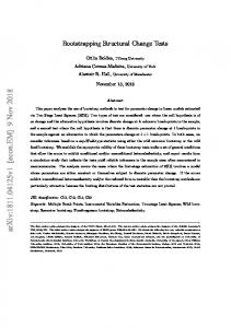
In this subsection, the size distortion when asymptotic distribution for the test statistics is used, is compared to the size distortion when bootstrap distributions are used. Simulation methods are used to show the graph of the true probability of rejecting the null hypothesis whereas the null hypothesis is true (size of the test), against the significance level of the test. For that purpose, the size of the tests are obtained by plotting the empirical distribution functions (EDF) of P values of the various neural tests (asymptotic and bootstrap ones). It should be noted that if a test is exact, i.e. the P value is based on the true distribution of the test statistic, then the plot of the corresponding EDF is represented by the 45o line. Consequently, the deviation of the P value EDF plots from the 45o line will be interpreted as an error in the test size. Figure 1 presents these test sizes in the case of the autoregressive parameters {ρj }4j=1 and ξ2 of the model 9 equal to −0, 5, for T = 100. 500 Monte Carlo replications are made, and 999 bootstrap replications are used for the bootstrap tests. A substantial distortion between the asymptotic tests size and the 45o line can be observed for all the underlying test statistics, particularly when the significant levels are lower than 10%, that are the levels usually chosen in practice. Conversely, there is size almost no size distortion with the bootstrap tests: the curves corresponding to the four bootstrap test are almost confused with the 45o line in Figure 1. The same graphs have been performed for T = 25, 50 and 200. The same results than previously are obtained. Even for T = 200, which is not small, an important loss of size equal to around 0.015 remains, when asymptotic tests are used, for a significant level of 0.05. Consequently, the use of bootstrap techniques is widely justified in our case, even when the samples sizes are not small.

4.3

Preliminary study under the null

All of the cases of the parameter values cannot be studied by Monte Carlo experiments. Consequently, the P value functions (PVF) are explored in order to select four interesting cases to study. The PVF is the true rejection probability of the null hypothesis, i.e. the true size of the test, for a significance level that is chosen to be equal to 0.05 here. The graphs of these functions can clearly underline the areas in the parameters space where bootstrap should behave more or less well according to their slopes and their curvatures. If the curve is steep with respect to a parameter in the neighbourhood of a point, this means that the statistic distribution depends on this parameter in this neighbourhood, thus, the statistic is not (locally) pivotal by definition. The only error in bootstrap P value (or critical values) calculation is due to the error in the parameter estimation under the null: since the statistic distribution is not exactly pivotal, an error in the parameter values leads to an error in the calculation of the distribution, and then, in the final P value (see Davidson [1998]). The steeper a curve is, the farther from a pivotal the statistic is, and more poor the bootstrap should be. As regards our preliminary experiment, we are interested in the variation of the 0.05 significance level PVF according to ξ2 , for different choices of (ρj )j . A parsimonious set of values for ξ2 , with more accuracy to the extremities, is considered: {−0.9875, −0.975, −0.95, −0.9, −0.8, −0.6, −0.4, −0.2, 0, 0.2, 0.4, 0.6, 0.8, 0.9, 0.95, 0.975, 0.9875}, and the various choices of (ρj )j are presented in Table 2. 10

Figure 2: P value functions of the asymptotic tests under the null for a confidence level of 0.05 Engle test 0.030 S i z e

0.025

. . . .. . .. ........... .......... ....... .. ........ ..... ... . . ... ... ...................... ... .. .. . ............... . ... ... . ... . .. .. ... ... ... .... ........... ...... ............. ... . . ..................................... . . . . . . . . . . . . . . . . . . . . . . . . . . . . . . . . .... . .. ..... ......... ....... ........ . . . ... ........ ............ ... ... . ... ..................... . .. ...... . .............. .. . ..... ....... ... ... ... . . . . . .......... . ......... ..... ........ ........ . ..... . ... ......... ...... ....... ........... .................... ...................... .............. ... ... ... ... .... ........... .... .... .... .... .... .... .... ............ ... ... ... ... ... ............. .... ........ .. .... .. .. ... ... . ...... ...... ... ...... ...................... ...... ........ ........ ........ .............. ... . . . . . . ................... . . . . . . . . . ........................................................ ... ......................... .. ..... ...... ... .... . . . . . . . . . ................ . . . . . . . . . . . . . . . . . . . . . . . . . . . . . . . . . . . . . . . ................... .. ......... .................. ................................................................

0.020 −1.0 −0.8 −0.6 −0.4 −0.2 0.0 0.2 0.4 0.6 0.8 1.0 ξ2 Péguin-Feissole test based on Kamstra specification 0.030 S i z e

0.025

. . . .. . .. ................. ...................................... .. . .... ................... ... . . ... .. . .... .. ... ... ... ... ... .. ......... .. ............ ...... . ... ... ... ... . . . .. . ............... ................. . . . . . . . . . . . .. . . . . . ........ ......... . ...... ... .............. . ...... ......... .. ....... ........ ........ ........ ........ ............... ... ... ... ... .... . ....... . ...... ...... ........ . . .... ... .. . . . . . . .. ............ ............... .... ....... ......... . ..... ... ................. .................................. ................. ................ ....... . . . ... .... .... .... ... ............. ... ... ... ... ............. .... . .... .... .... . ........ ..... .... ...... .. .... ...... . ................ .... . . . . . . . . . . . . . . .................... . . . . . . . . . . . . . . . . . . . ...................................... ...................... .. .................................................. ...... ...... .......... . ...... ...... . . . . . ............ . . . . . . . . . . . . . . . . . . . . . . . . . . . . . . . . .................... .... ...... . ............. ............ . . . . . . . . . . . . . . ................ .................................

0.020 −1.0 −0.8 −0.6 −0.4 −0.2 0.0 0.2 0.4 0.6 0.8 1.0 ξ2 Péguin-Feissole test 0.035 S i z e

0.030

.... ....................... ................................................. .................... ......... ....... ................................................................ ... .................................................. ........ .... ............ . ........ ........ ......................... ... .... ... . ........ .............. . .. ... ... .... ... ........ .. . . . ...... ... ...... ...... .............. ...................... ...... . ........... . .... ...... . .... ........ ........ ................ .......... .. ..... ... .. ..... . . .............. ......... ......................... ..... ......... ... ... ... ....... ... ... ... ... ... ... ... ... ... ... ... ... .......................... ......... ........ ........ . . . ......... .. .... . . . . . . . . .. . . . . . . . . . . . . .. . . . . . . . . . . . . ..... ........ ........ .... ........ ..... ... . .. .. . . . . .. . . . . . . . . . . .. ...... .... ... ... ... ... ... ... . .... . ........ . .. . .. . .. . .. . .. . .. ..... .. . ..... ... ... ... .. .... .......... .. .... .. .. ... ... .... . ................ ..... ...... ........ . ..... . . ..... .... .... ...... .... .. ...... ........... . ........ ... ...... ..................... ........ .. . ........ . . . . . . . . . .. . . ......

0.025 −1.0 −0.8 −0.6 −0.4 −0.2 0.0 0.2 0.4 0.6 0.8 1.0 ξ2 ................................ ........ ........ .. ...... ...... ...... .. ... ... ... ... ... ... .. ....... .............

Case Case Case Case Case Case

1 2 3 4 5 6

: : : : : :

ρj = 0.9 ∀j ∈ {1, . . . , 4} ρj = 0.5 ∀j ∈ {1, . . . , 4} ρj = 0 ∀j ∈ {1, . . . , 4} ρj = −0.5 ∀j ∈ {1, . . . , 4} ρj = −0.9 ∀j ∈ {1, . . . , 4} ρ1 = −0.9 ρ2 = −0.5 ρ3 = 0.5 ρ4 = 0.9

11

Table 2: Values of Parameters ρj for the preliminary study Case Case 1 Case 2 Case 3 Case 4 Case 5 Case 6 (mixed)

Parameter Values ρj = 0.9 ∀j ∈ {1, . . . , 4} ρj = 0.5 ∀j ∈ {1, . . . , 4} ρj = 0 ∀j ∈ {1, . . . , 4} ρj = −0.5 ∀j ∈ {1, . . . , 4} ρj = −0.9 ∀j ∈ {1, . . . , 4} ρ1 = −0.9 ρ2 = −0.5 ρ3 = 0.5 ρ4 = 0.9

Figure 2 presents the PVFs, constructed using the asymptotic neural test, with respect to ξ2 , for T = 100 and by carrying out S = 10, 000 Monte Carlo replications for each value of ξ2 . Each PVF corresponds to a particular choice for (ρj )j . It should be noted that if a test of 0.05 level performs correctly, the corresponding PVF should be close to the 0.05 horizontal line. We observe a substantial underrejection which is lower than 0.025 in all the cases under consideration, i.e. twice lower than the significance level 0.05! Therefore, the asymptotic approximation performs poorly in all the cases, which confirms the results of the first study and greatly justifies the use of bootstrap techniques. The graphics in Figure 2 are used to decide which cases of the parameter values, ξ2 and {ρj }j , to investigate in depth 6 , and the selected cases are presented in Table 3. Table 3: Chosen parameter values for Monte Carlo simulations Case 1 2 3 4

parameter values ρj = −0.5 ∀j and ξ2 = −0.5 ρj = 0.9 ∀j and ξ2 = −0.95 ρj = −0.9 ∀j and ξ2 = 0.85 ρj = −0.5 ∀j and ξ2 = −0.5

Error terms ∼ N (0, 1) ∼ N (0, 1) ∼ N (0, 1) ∼ t(5)

Case 1 is chosen as a reference case, for which bootstrap tests might not encounter problems, because the curvature of the graphs is flat according to ρj and ξ2 . It means that the statistic is locally pivotal for these parameters values, and the size distortion will be small. Cases 2 and 3 are deliberately chosen to be those for which bootstrap tests might encounter problems because the PVFs display considerable curvature. Finally, case 4 was chosen with the same parameters as in case 1, but with error terms conditionally distributed as t(5) distribution, instead of N (0, 1).

4.4

Results under the null

In this subsection, the results relative to the size of the various tests are presented in the case where the data are generated from homoskedastic models. More precisely, the graphs 6

It is also possible to plot the same PVFs against ρj for different values of ξ2 .

12

Figure 3: Size of the neural tests for a confidence level of 0.05 Case 1 of the parameters (nonproblematic case) Tests based on the linear specification 0.08 S i z e

0.06 0.04 0.02 0.00

.. ....... ... . .... ...... ...... ...... .. .. ..... . . .. ... . .. ... ..... ..... ............................... ... ...... . . . ....... .... . . . . .. . .... . .. ...... ...... ...... . . ... ... ................................................................................................................................................................................................................................................................................................................................................................................................ . . . . . . . . . . . . . . . . . . . . ... . . .. . ..... ........... .... ....... .... .... ..... ...... . ......................... . ..... ... ..... .... ... .. ..... .. .... ... .... .... ..... ...... ....... . .. .......... ...... . . . . .. ...... ...... . . . . . . . . . . . . . . . . . . . . . . ......... ..... .... ...... ..... ......................... .......... ..... ...... ........ ..... ........... ..... ................. .......... ..... ....... ............. ................. . . . . .. . . . . . . . . . . . . . . . ... ..... ... .... ... ...... ...... .. .. .... ............... . . . . . . ..

0

40

80

120

160

200

Sample Size Tests based on the Kamstra specification 0.08 S i z e

0.06 0.04 0.02 0.00

... ........ . ....... ....... .... ...... ... ...... ... . . . ........... ...... ...... ... . ........ . . . . ... . . . . . ....... .. ... . .... ... ... ............ .... .. . .. ...... ..... .............................................................................................................................................................................................................................................................................................................................................................................................. . ........ ... ...... .. ............ ... .. . ..... ... .... .. ..... .... ........... ...... ...... ... . ..... . ..... .. ...... ... ... ...... .... ..... . .. ..... .... ....... ..... ..... ........ ...... ... ... . . . . . ..... . .. . ... ........ ..... . . . . . . . . ....... ..... .. ..... ...... ..... ...... ................... ..... .................. .................................... ..... ...... ......... ............ ..... .......... .......... . .................. . . . . . ..... .................. ..... ....................... . . . . . ........ .. ...... ......

0

40

80

120

160

200

Sample Size Tests based on the nural specification 0.08 S i z e

0.06 0.04 0.02 0.00

..... . . ...... ... . .. .... ... . . . .. . ..... . . ... ... . ... .... ...... .... ... ... ...... ..... ... . . ...... .. . . .. . .. ..... ........................................... .... .. ..... ...... ...... ... .... ... . ... .. ... . ........ ............................................................................................................................................................................................................................................................................................................................................................ . . .... ... . .. . . . . . . . . . . . . . . . . . . . ... .... ......... ......... .. ...................... .............................. ........ . .......... ......... ... . ...... . . . . . . . . . . . . ......... . .. .. ........ . ..... ....... . .... ....... ... .. .... ...... ..... ................................................................... ..... ..... ............ . . . . . . . . . ................. ............ ... ... ........... .. ..... ............. . . . . . ... . ....... ... .. ......... ..

0

40

80

120

Sample Size ................................ ........ ........ .. ...... ...... ...... .. ... ... ... ... ... ... .. .......

Asymptotic test Parametric bootstrap test (b0 ) Nonarametric bootstrap test b1 Nonarametric bootstrap test b2 Nonarametric bootstrap test b3

13

160

200

Figure 4: Size of the neural tests for a confidence level of 0.05 Case 2 of the parameters (problematic case) Tests based on the linear specification 0.08 S i z e

0.06 0.04 0.02

.... .. . . .... .. .................. ... ....... ... .... .. . .... ........... ...... ...... ... . . .. ...... ...... .... .. ...... .... ......... ... ...... . . . . . . . . . ........................................................................................................................................................................................................................................................................................................................................................ . ... ... .. ... ...... ... ...... ....... ................ ... ....... .. ... ... . ..... ........ ........ . .............................. . ... .......... . . . ....... ... ....... . ..... . . . ....... . . . ..... ....... ... ....... . . . . . ... . . . . . . . . . . . ..... ....... ..... .. .. ..... ................. ........ ......... ............................ ..... ..... .....

0.00 0

40

80

120

160

200


0.06 0.04 0.02

.. .. ... .......... .. .............. .. . ...... ..... ...... ...... ......... ............. .. .... ..... ... .... .. . .. ...... .. ..... . ................................................................................................................................................................................................................................................................................................................................................................................... . .......... ... . . ...... . .. .. ............. . . . . . ....... ..... . ..... ....... ... .. ...... . . .................................. . . ... ......... . . . . . ........ ... ....... . ..... . . . . . . ........ ..... ..... ..... ........ ... ....... ..... ........ ....... ......... .. . . . . . . . . . . . . . . ........ ..... ........ . ........ ........................ ....... ..... .....

0.00 0

40

80

120

160

200

Sample Size Tests based on the neural specification 0.08 S i z e

0.06 0.04 0.02

. ... . . ... ... ... . . .. ...... ......... .. .... .. ... ... ........ ...... ..... ..... ........................ .... . . . ... ........ .... .... .. . . . . ... . ..... ...... . . . ......................................................................................................................................................................................................................................................................................................................................................... . ... ...... ...... ... . . . . . . . . .... .. . .... . . ... . . . ........ ........ ...... .............................................................. ........... ...... ...... ..... ..... ...... ..... ...... ......... ........... ..... . ..... ................................. . . . . . . . . . . . . ..... . .................................................. ..... .... ....

0.00 0

40

80

120

Sample Size ................................ ........ ........ .. ...... ...... ...... .. ... ... ... ... ... ... .. .......


14

160

200

Figure 5: Size of the neural tests for a confidence level of 0.05 Case 3 of the parameters (problematic case) Tests based on the linear specification 0.08 S i z e

0.06 0.04 0.02

. ..... ..... . ..... ... .... ..... . ... ..... ... .... ... . . . . . ... . ...... ..... . ... .... ... ...... . .. ..... .... ........ ... ................................................................................................................................................................................................................................................................................................................................................................. ... .......... ..... .. ...... ..... ........ . . . ...... . . . . . . . . . . . . . ... ... ..... . .. . .. ..... ...... ... ................... ... ..... ..... . ... . ... . . .. . .. ...... ............. ................... ....................................................................... ... ...... ........ ....... ... .............. ...... ............. . ........... ... ... ...............

0.00 0

40

80

120

160

200


0.06 0.04 0.02

. ..... ..... . ..... ... .... ..... . . . . ..... .... .... ... . . . . .. . ... . ...... .... . ... .... . .. .... ...... . ..... .... ...... ... ................................................................................................................................................................................................................................................................................................................................................................ .. ... .. ......... .... .. . .. .. ..... .. ... . ............ . ........ ...... .. . ..... .. ... ...... .. .. ... ...... ...................... ..... ... . ...... . ..... . ... . . . . . ... .......... ................... ............ ........................................... .............. ............ ......... .. ....... ............... ....................... ....... ... . ... ...............

0.00 0

40

80

120

160

200

Sample Size Tests based on the neural specification 0.08 S i z e

0.06 0.04 0.02

.. . .... .. ..... ...... ...... ...... ... ... . ...... ... .... ..... ..... ........... . ..... .... . .. .. ... ........ . ... ..... .................................................................................................................................................................................................................................................................................................................................................................... . .. . .......... . . . . . . . . . . . . . ..... . ........... .. . ...... .... ..... ....... .. ...... ...... .... .... ..... ....................... ............................... . .. . ..... ... ..... . . . ......................... ..... .... ...... ...... ... ...... . ..... . . ................... . . . . . ...... .. .. ..... ....... ... ...... ..... ..... ........... ... ....... ...............

0.00 0

40

80

120

Sample Size ................................ ........ ........ .. ...... ...... ...... .. ... ... ... ... ... ... .. .......


15

160

200

Figure 6: Size of the neural tests for a confidence level of 0.05 Case 4 of the parameters (student case) Tests based on the linear specification 0.18 0.16 0.14 0.12 S i z e

0.10 0.08 0.06 0.04 0.02 0.00

... ...... ...... ...... . ...... ...... ...... . . ...

. ..

. ...

. ...

...... ...... . ...... .. ......

........... ..... ............... .... ........ .... ... . . . ..... .... . . . ... . . . ... ..... ..... .... ..... . . .... . . . . . . . .... . . ..... .. ... .... ......... ..... .. ... . ... ................................... . .. ... .... .......... . . . . . ... ........ ... ... ..... ... ... .. ... ..................... ... ... .. .. ... ... . .. .. . .. . . . . ...... ... . . ... ... ..... ...... .. .. . .. . ... . ...... .. .... .. .... ..... . . ..... ... . . ... ...... . .. . ... . . .. .... . . . . . . ...... . . . . . . . ........ ... ... .... ...... ...... ..... .. .. .. ... .. ....... ... ...... . . ... ..... .... ..... ..... . . . . . . ... .. ............. . . . ... ... .... ... .. ..... . . . . . . . . . . . . . . . . . . . . . . ..................................................................................................................................................................................................................................................................................................................................... . .. ... . . . . . . ... ........ ........ ... ....... ... .. . ... .. .. ... . . . ... .... .. .... ........ .. . . . . ....... . .... . ..... . . ..... ..... ..... ... . . . . . . . ...... ... ..... ..... . ... .... . ... .....

0

40

80

120

160

200

Sample Size Tests based on the Kamstra specification 0.18 0.16 0.14 0.12 S i z e

0.10 0.08 0.06 0.04 0.02 0.00

...... ...... ...... ...... ..... ...... ..... . ......

. ..

. ...

. ...

. ..

. ...

..... ... ... .. .... . .....

..... .... ............. ....... ..... ....... ..... ...... .... . . . . .... . . . .. . . . . .... . . . ... .... ..... ..... ..... .... .... . . . . . ... .... ... .... ... .............................................. .... .... ....... ... ..... .. ........ . . . . . . . ..... . .. ..... .. .... ... ..... ... ........................ .. .. . .. ... .. .... . .... .. ... .. . ... . . .. ... ... . .. . .... ... .. .... ... ... ..... ... .... .. .. . ..... ... .... . .. . . .. . . . .. ...... .......... ... ... ..... . .. . . . .... . . . . . . . . . ... ... .. ... ... . . ..... . ... ..... .. ..... .. .... . .. . .. .. . .. .. ...... ... ....... .. .... .... .. ...... ..... . .. . . . . . . . . . . . . . . ................................................................................................................................................................................................................................................................................................................................................. . . . . . ..... . . . . . .. ........ ....... ... .... ... .. . ... ... ... ... . . . .. .... ..... ... .. ... . .. ......... . .... ... .. .... ...... .. ...... ...... .. . .... . . . . ... .... . . .. .....

0

40

80

120

Sample Size

16

160

200

Tests based on the neural specification 0.18 0.16 0.14 0.12 S i z e

0.10 0.08 0.06 0.04 0.02

..... . . ..... . ..... . ... . ............. ..... .... ... ........... . .... ... ... . .. . ... ... ... .. ... ..... .. . . . . . . .. ... .... ... .. ... .... . ... . ... ... .... .......... ... ..... ...... .. .... .... .. .. .. .. .... . ... ... .. ... .. .. ..... . ... . ... ... ... . ... .. . .............. . .. . ... . .. .. ... . ... .. .. . ... .. .. ... ... .. .. .... . .. .... .. ...... ... .... .... . . ... .. ..... ... ... .. .. ... .... .... .... .. .. . . . .. ......... ... . .. ........... .... ... .. .... .. . . . . ... .. . ..... . . .. . ... .. .. ... . . . . . . .... . . . . . . .. ..................... .... . . . .. .... .. .. ... . ........ .... .... .. ... .. ..... ..... . . .. .. .... ... . . . ................................................................................................................................................................................................................................................................................................................................. .. .... ...... ...... . .. ... ......... .... ... ...... .. ... ... ... .. . ... ... ... .... . . . . . ...

0.00 0

40

80

120

Sample Size ................................ ........ ........ .. ...... ...... ...... .. ... ... ... ... ... ... .. .......


17

160

200

show the proportion of Monte Carlo replications with P values less than 0.05 (being an estimate of the test size) for each test of Table 1, as a function of T . The simulations are carried out for all the cases of the parameters given in Table 3 and for sample sizes between 10 and 200. For each experiment, the number of Monte Carlo replications S is equal to 1000, making standard error of the tests size estimates equal 0.0069 for 0.05 size, the maximum standard error being 0.016 (if size is equal to 0.5). Using large value for B is necessary to avoid a power loss, and so, the number of bootstrap replications B is taken equal to 999 7 . The results are presented in Figures 3–6. The results obtained by the Kamstra [1993] variants test are quite identical with those of the Engle test. Moreover, the curves obtained have a similar look to those obtained with the neural tests. As expected, performance of asymptotic tests is very poor. We observe that all the bootstrap tests, with or without neural networks, perform well in all the cases under consideration, even for cases 2 and 3, which were likely to encounter problems. Obviously, parametric bootstrap tests (as well as asymptotic tests) do not perform satisfactorily in the case where the error terms are nonnormally distributed, for which an important overrejection is observed.

4.5

Results under the alternatives

For comparing the power of the various tests, the results are presented using the graphical presentation of Davidson and MacKinnon [1993, 1998a] which yields graphs easily interpretable. These curves represent the plot of power of the tests against a corrected size that corresponds to the true probability of rejection of the null hypothesis when the null is true (i.e. the significance level). We will call this power the true power. The basis of these graphs is the EDF Fˆ (x) of the P values associated with the simulated realizations of a test statistic. The X-axis represents Fˆ , which are the EDF when the data are generated under the null hypothesis, and the Y-axis represents F ? , which are the EDF when the data are generated under the alternative. The size-power curves are therefore generated on a correct size-adjusted basis. According to theoretical results, the power of a bootstrap test would be very similar to that of the corresponding asymptotic test, on the basis of this size correction. If we consider that the size distortions are well corrected by bootstrap, we check here that the method does not involve any power loss or any instability. However, there is no unique way to measure the power with respect to the adjusted size in a Monte Carlo experiment: there is an infinite number of Data Generating Processes (DGPs) that satisfy the null hypothesis. Since the test statistics are not pivotal, the choice of the DGP used to correct the size can matter greatly. Davidson and MacKinnon [1996] argues that a reasonable choice is the pseudo-true null, which is the DGP that satisfies the null hypothesis and is as close as possible, in the sense of the KullbackLeibler Information Criterion, to the DGP used to generate Fˆ1 ; see also Horowitz [1994, 7

We propose a number of bootstrap replications such that (B + 1)0.05 is an integer. The reason comes from the computation of critical values for a test of significance level of 0.05. Taking B such that (B + 1)0.05 is an integer permits to have the 0.05 and the 0.95-quantiles in the set of bootstrap replications of the statistic. In the case of P values, it is important only for taking decision for significance level 0.05, see Davidson and MacKinnon [2000]. What is really important in our case, for computing the P value, is the number of bootstrap replications that must be taken as large as possible to take into account the excess of kurtosis in one or both of the tails of the distribution of the statistic, see Davidson and MacKinnon [2000] and Andrews and Buchinsky [1997].

18

1995]. The pseudo-true null is used in our experiments. For calculating it, we compute the average of estimates of the series under the null of homoskedasticity. The simulations are done with 1000 replications under the alternative, 2000 replications under the null (for correcting the power), B = 999 and T ∈ {25, 50, 100, 200}. The maximum standard error for the power estimations is equal to 0.016. The computation of the rejection probability is the same as under the null hypothesis, except that now, the data are generated under the alternative hypothesis and that the size test is corrected. The alternative hypothesis is represented by various conditional heteroskedastic models chosen to illustrate a variety of situations, see Table 4. The parameter α ¯ in Table 4 can be used to reflect the distance from an alternative to the null hypothesis. We take α ¯ in the set {0.1, 0.2, 0.3, 0.4, 0.5, 0.6, 0.7, 0.8, 0.9}. The parameters of the conditional mean regression are chosen following the four cases determined by the preliminary study (see Table 3). Figures 7–7 present the estimates of corrected size-power curves for the asymptotic and bootstrapped neural tests, as well as for the asymptotic and bootstrapped Engle tests. Since the results for the bootstrap tests are satisfactorily for all the cases of the regression parameters, we restrict the presentation of the results to the case 2 of the regression parameters (Table 3) that would be problematic for bootstrap techniques. We take δ = 1, α ¯ = 0.5 (medium heteskedasticity), and T = 200. Figure 7 presents the curves for the Gaussian ARCH(3) alternative, that will be used as a reference case for comparison. It can be observed that the neural tests are less powerful than the tests for the linear specification. This feature was expected since the neural tests are more robust that the other ones. The neural tests based on Kamstra specification are more powerful than the “classical” neural tests (but less robust due to the squared specification of the lags). In any way, the bootstrap tests perform correctly, since the true power curves of the bootstrap tests are confused with the true power curves of the corresponding asymptotic tests. This prooves that the test size is satisfactorily corrected by the bootstrap techniques (see subsection 4.4) without loss of true power. Figure 8 presents the curves for the Gaussian IARCH(3) alternative. Even if there is a unit root in the conditional variance specification, the tests performs correctly and the same remarks than previously hold about the tests, except that they have a much greater power than in the case of covariance stationary ARCH error terms. Figure 9 presents the curves for the Gaussian ARCH(1) alternative. The weight of the heteroskadasticity remains α ¯ = 0.5 as previously, but this weight is totally localise on the parameter α1 rather than being shared amoung α1 –α3 . The results are correct. Figure 10 presents the curves for the Gaussian ARCH(5) alternative. There is a general loss of power for all the tests since they are specified for three lags and they are not able to detect the heteroskedasticity of order 4 and 5. Figure 11 presents the curves for the Gaussian log-ARCH(3) alternative. The performance of the test is quite good. Figure 12 presents the curves for the Gaussian NARCH(3) alternative. We choose the nonlinear parameter δ equal to 0.1 (if δ = 1, it corresponds to a linear ARCH model). Figure 14 presents the curves for the Gaussian max ARCH(3) alternative number 3.3. Figure 14 presents the curves for the Gaussian TARCH(3) alternative number 4.1. In the case of this strongly nonlinear specification, the classical linear specifications fail to detect ARCH effect. The neural specification keeps a certain power. Again, the bootstrap tests keep their true power.

19

Table 4: Heteroskedasticity types

Model

Name

Conditional Variance ht

1.1

ARCH(3)

(1 − α ¯ ) + α2¯ ε2t−1 + α3¯ ε2t−2 + α6¯ ε2t−3

1.2

IARCH(3)

0, 2 + 0, 4ε2t−1 + 0, 3ε2t−2 + 0, 3ε2t−3

2.1

ARCH(1)

(1 − α ¯) + α ¯ ε2t−1

2.2

explosive ARCH(1)

0, 2 + 1, 4ε2t−1

2.3

ARCH(5)

3.1

log-ARCH(3)

3.2

NARCH(3)

3.3

“max-ARCH(3)”

max 1 − α ¯ , α2¯ ε2t−1 , α3¯ ε2t−2 , α6¯ ε2t−3

3.4

ARCH(3) “in log.”

ln 1 + (1 − α ¯ ) + α2¯ ε2t−1 + α3¯ ε2t−2 + α6¯ ε2t−3

3.5

“fractional” ARCH(3)

4.1

TARCH(3)

(1 − α ¯ ) + α2¯ I(εt−1 ≥0) + α3¯ I(εt−2 ≥0) + α6¯ I(εt−3 ≥0)

4.2

TARCH(3)

(1 − α ¯ ) + α2¯ ε2t−1 I(εt−1 ≥0) + α3¯ ε2t−2 I(εt−2 ≥0) + α6¯ ε2t−3 I(εt−3 ≥0)

4.3

4.4

TARCH(3)

symmetric TARCH(3)

(1 − α ¯ ) + α3¯ ε2t−1 + h

exp (1 − α ¯) +

α ¯ 2

α ¯ 2 ε 3.5 t−2

+ α5¯ ε2t−3 +

ln(ε2t−1 ) +

α ¯ 3

α ¯ 2 ε 7.5 t−4 α ¯ 6

ln(ε2t−2 ) +

+

(1 − α ¯ ) + α2¯ (ε2t−1 )δ + α3¯ (ε2t−2 )δ + α6¯ (ε2t−3 )δ

2 (1 − α ¯ ) + α2¯ ε2t−1 + α3¯ ε2t−2 + α6¯ εt−3

     (1 − α ¯ ) + α2¯ ε2t−1 + α3¯ ε2t−2 + α6¯ ε2t−3     16      (1 − α ¯ ) + α2¯ ε2t−1 + α3¯ ε2t−2 + α6¯ ε2t−3     16

i1/δ

o

h

h

i

ln(ε2t−3 )

h

n

α ¯ 2 ε 15 t−5

i

i−1

if εt−1 ≥ 0 otherwise if ε2t−1 ≥ 1 otherwise

5.1

Student ARCH(3)

Model 1.1 with Student errors terms

5.2

Student TARCH

Model 4.3 with Student errors terms

20

Figure 7: “True” power curves of the tests Case of Gaussian ARCH(3) alternative, with weight 0.5 (T=200)

1.00 0.80 P o w e r

0.60 0.40 0.20

Linear specification

Kamstra specification

....................... .......................... ................ ........................... ...................................... .......................... ............. ........... .............. ..... ............. ........... ............ ..... .......... .......... ..... .......... ................ ..... . . . . . . .. . . . . .... ....... ........... ..... .......... ..... ..... ....... ......... ..... . . . . . . .... ...... ..... ... ..... .... ..... .... ..... . . . ...... . ..... ... ..... ... ..... ... ..... ..... .... . . . ...... . ..... .... ..... ..... ..... ..... .... ..... . . ..... . .... . ..... .. ..... .... ..... . ..... . . . .... . .... . ..... .. ..... .... ..... . ..... . . . .... . ..... .. ..... ..... .. ..... . .... . . . . ..... ..... ..... ..... ..... . . . .... ..... ..... ..... ..... . . . . . ..... .... ..... ..... ..... . . . . .....

........................ ............................. ...................................... ........................................... .............................. ............... ............ ........... ..... ............... ............... ..... ...... .. .............. ..... ............. ................ ..... . . . . . . . .. . . ... .... ............ ..... .......... ..... ........ ..... ...... ..... . . . ....... . .... ..... ..... ... ..... ..... .... ..... . . . ........ . ..... .. ..... ... ..... .... ..... ... .... . . . ...... . ..... ... ..... ..... ..... ..... .... ..... . . ..... . .... . ..... ... ..... ... ..... ..... . . . ... . .... .. ..... .. ..... ... ..... ..... . . . .... . .. ..... ..... .. ..... ..... .. .... . . . . ..... ..... ..... ..... ..... . . . .... ..... ..... ..... ..... . . . . . ..... .... ..... ..... ..... . . . . .....

0.00 0.00

0.20

0.40

0.60

0.80

1.00

0.00

0.20

0.40

Corrected size

0.60

0.80

Corrected size

Neural specification 1.00 0.80 P o w e r

0.60 0.40 0.20

.... ............. ............ ..... ............ .... ................... ......... . . . . . . ............. ..... .......... .. ..... ............ ..... ....... .... ..... ............ .... . . . . . . . . .... .. .... ........ ..... ....... .. ..... ..... ......... .. ...... ..... ..... . . . . . . . . . . . ..... ... .... .......... ... ..... ....... ... ..... .... .. ..... .... .... ..... . . . . . . . . . . . . . .... ..... ... ..... ....... .. ...... .. ... ..... ..... ...... ..... ...... ..... . . . . . . . . . . .... .... ..... .... ..... ..... .... ..... ..... ..... .... .... .... . . . . . . . . . ..... ... ... ..... .... . ..... ... .. ..... .. .. ..... .. ... . . . . .... ... . ..... ... .. ..... ... .. ..... .. .. ..... . . . .... ... . .... ..... ... .. ..... .. . .. .. ..... ..... ... ... . . . . . ..... .... ... ..... . ..... ..... ..... ... .... . . . ...... . .. . ..... ..... .. ..... .. ..... .. ......... ... .....

0.00 0.00

0.20

0.40

0.60

0.80

Corrected size

21

1.00

................................

45o line

................................

Asymptotic test

...... ...... ...... ..


.............


.......


.


.

.

.

1.00

Figure 8: “True” power curves of the tests Case of Gaussian IARCH(3) alternative (T=200)

1.00 0.80 P o w e r

0.60 0.40 0.20



................................................................................................................................................................................................................ ..................................................................................................... ................. ........ . ........ ..... ..... ..... ..... ...... ..... . .. . . .... . ..... .. ..... ..... .. ..... . . ... . . .... . ..... .. ..... ..... .. ..... . . ... . . ..... .. ..... ..... ... ..... .... . . . . ..... ..... ..... ..... ..... . . . .... ..... ..... ..... ..... . . . . .... ..... ..... ..... ..... . . . . ..... ..... ..... ..... .... . . . . ..... ..... ..... ..... ..... . . . .... ..... ..... ..... ..... . . . . . ..... .... ..... ..... ..... . . . . .....

................................................................................................................................................................................................................................... ............................................................................................ .......... .......... ..... ...... ..... ..... ...... ..... . . . .. .... . ..... .. ..... ..... .. ..... . . . ... . .... ..... .. ..... .. ..... ... ..... . . . . ..... .. ..... .. ..... .. ..... .... . . . . ..... ..... ..... ..... ..... . . . .... ..... ..... ..... ..... . . . . .... ..... ..... ..... ..... . . . . ..... ..... ..... ..... .... . . . . ..... ..... ..... ..... ..... . . . .... ..... ..... ..... ..... . . . . . ..... .... ..... ..... ..... . . . . .....

0.00 0.00

0.20

0.40

0.60

0.80

1.00

0.00

0.20

0.40

Corrected size

0.60

0.80

Corrected size


0.60 0.40 0.20

............. ............... ............ .......... ............................ ... ............................................ .... ............................ .............. ..... ............................... ... . . . . .. . . . . . .... . . . . . . . . . . . . . . ........ ............... ... . . . . .. . . . . . . . . . . . . . . .. . . . . . .. . .... ....... ...... ..... .......... .... ..... .......... .... .... ........... ..... .... ..... . . . . . . . . . . . . . . . . . . .... ..... ... ..... ..... ... ... ..... ... .. ..... .. .. .... . . . . ... . . .... .. .. ..... ... ... ..... .. ... ..... .. ..... . . . . . .... ..... . .. .... .. ... ..... ..... .. ..... . . ... . . .... .. ..... ..... .. ..... .. ..... . . . . . .. ..... ..... .. ..... .. ..... .... . ... . . . .... . ..... .. ..... .. ..... ..... . ... . . . . ..... .... .. ..... ... ..... ..... . .. . . . .... . ..... ..... ..... ..... . . . . ..... ..... ..... ..... .... . . . . ....

0.00 0.00

0.20

0.40

0.60

0.80

Corrected size

22

1.00

................................

45o line

................................

Asymptotic test

...... ...... ...... ..


.............


.......


.


.

.

.

1.00


1.00 0.80 P o w e r

0.60 0.40 0.20



............. ................................................ .................................................................. ......................................................... ........................... . ............. .................. ............. ........ ........ ....... ..... ........ ......... .......... ..... ........... ..... ............ ..... ........ . . . . . .. . .... ... . ..... .. .. ..... .. . ..... .. . ..... . . . ...... . .... .. ..... ... ..... .... ..... ..... ..... . . . .... . ..... .. ..... .. ..... ... ..... .... . . . ... . ..... .. ..... .. ..... ... ..... ..... .. . . . .... ... ..... ..... .. ..... ..... . ... . . . .... .. ..... ..... ..... ..... . . . . ..... ..... ..... ..... .... . . . . ..... ..... ..... ..... ..... . . . .... ..... ..... ..... ..... . . . . . ..... .... ..... ..... ..... . . . . .....

............... ................................................. ................................................................ ...................................................... ........................ ............... . .................... ............ ....... ........ ......... ..... ............ .............. ..... ................... ..... .......... ..... . . . . . . .... ... .. .. . ..... .. .. ..... ..... ... .. ..... . . . ....... . .... ... ..... ... ..... .... ..... .... ..... . . . . .... ..... ... ..... .. ..... ... ..... .... . . . ... . ..... .. ..... .. ..... ... ..... ..... .. . . . .... . ..... .. ..... .. ..... ..... . ... . . . .... . . ..... ..... ..... ..... . . . . ..... ..... ..... ..... .... . . . . ..... ..... ..... ..... ..... . . . .... ..... ..... ..... ..... . . . . . ..... .... ..... ..... ..... . . . . .....

0.00 0.00

0.20

0.40

0.60

0.80

1.00

0.00

0.20

0.40

Corrected size

0.60

0.80

Corrected size


0.60 0.40 0.20

................... ....... ........... ............... .. .............. ....... ..... ............. .............. ..... . . . . . . . . . . . . . . ... ......... ....... . . . . . . . . . . . . . . . . .... .... ......... .. ..... .. . .. ........... ..... ..... ........ ... . .. ..... ........ ..... ........ ...... . . . . . . . . . . ..... .......... ... ..... ... .... ..... ...... ...... ..... ...... .. .... ........ . . . . . . . . . . . . .... ....... ... ..... ..... ... ..... ...... ... ..... ..... ... ..... ...... . . . . . . . . . . ... . ..... ..... ... .... ... .... ..... ... ..... .. .. ..... . .... . . . . . . . . .... ..... .. ..... .. ..... ... .. .. ..... .. ..... .. . . . . . ... ..... .. .. ... ..... .. ..... .. .. ..... ... .. .... . . . ... ... . .... .. . ..... .. .. ..... .... ... ..... ..... . . . .... .. . ..... .. . .... .. ... ..... . ..... ..... . ... . . . .... .. ..... ..... .. ..... .. ..... . . . ... . ..... .. ..... ..... ..... .... . . . . ....

0.00 0.00

0.20

0.40

0.60

0.80

Corrected size

23

1.00

................................

45o line

................................

Asymptotic test

...... ...... ...... ..


.............


.......


.


.

.

.

1.00


1.00 0.80 P o w e r

0.60 0.40 0.20



........... ......................... ................ ........... .................. .............. ........ .... .............. ............ ........... ..... ...... ........... ........ ..... .......... ....... .......... ..... ....... . . . . . . . . . . . . . . .. ... ........ .... ..... ..... ......... ........... ..... ..... ......... ........... ..... . . . . . . . . .. .... ..... ..... ...... ..... ..... ..... ...... ..... ....... . . . . . . .. ..... ...... ..... ..... ..... ... ..... ... .... . . . ....... . ..... ... ..... .... ..... ..... ..... ... ..... . . . ....... .... ... ..... ... ..... .... ..... ... ..... . . . . .... .... .. ..... .. ..... ... ..... . ..... . . ... . . ..... .. ..... ... ..... ..... .. .... . ... . . . ..... .. ..... ... ..... ..... .. ..... . . . .... ..... ..... ..... ..... . . . . . ..... .... ..... ..... ..... . . . . .....

.......... ......................... ............... ............. .................. .......... ....... .... .............. ............ ......... ..... .......... ........... .......... ..... ............... ....... ..... ........ ... . . . . . . . . . . . . . . . . ...... .... .............. ..... ....... ........... ..... ........ ..... .......... ..... . . . . . . . . . . .. .... ..... ..... ....... ..... .... ..... ...... ..... ......... . . . . . . ..... ....... ..... ...... ..... .... ..... .. .... . . . ....... . .. ..... ..... ..... ..... .... ..... ... ..... . . . ....... .... ..... .... ..... ... .... ..... ... ..... . . . ..... . .... . ..... .. ..... ... ..... . ..... . . ... . . ..... .. ..... ... ..... ..... .. .... . . ... . . ..... .. ..... ... ..... ..... .. ..... . . . .... ..... ..... ..... ..... . . . . . ..... .... ..... ..... ..... . . . . .....

0.00 0.00

0.20

0.40

0.60

0.80

1.00

0.00

0.20

0.40

Corrected size

0.60

0.80

Corrected size


0.60 0.40 0.20

....... ........... ........... ..... .......... ......... . . . . . . . . . . . ............ ........ .......... ... ........ .............. ..... ............ ..... ............... . ..... . . . ..... ............. . . . . . . . . . ..... ........ ............ ..... ...... .. ..... ...... ... ..... .... ......... . . . . . . . . .... ..... .... ..... ......... ..... ...... ... ..... ..... .. ..... . ..... ... . . . . . . ..... ..... ... .... .... .. ..... ..... .. ..... ...... ... ..... . ...... .... . . . . . . .. .... .... ... ..... ..... .... .. ..... ...... .. .... .... ..... . . . . . . . . .... . ..... .... .. ..... .... .. ..... ..... .. ..... ... ... .... . . . . . . .... .... .. ..... .... .. ..... .... .. ..... ... .. ..... . .... ... . . . . . . ..... ... .. .... .. . ..... .. .. ..... .. .. ..... . . . . ... .. .... .. . ..... .... ..... ..... ..... ... ..... . . . ...... . .... . ..... .. ....... ... ........ . . . . ....

0.00 0.00

0.20

0.40

0.60

0.80

Corrected size

24

1.00

................................

45o line

................................

Asymptotic test

...... ...... ...... ..


.............


.......


.


.

.

.

1.00

Figure 11: “True” power curves of the tests Case of Gaussian log-ARCH(3) alternative, with weight 0.5 (T=200)

1.00 0.80 P o w e r

0.60 0.40 0.20



......................................................................... ........................................................................................................................................................... .......................... ................. ............ ....................... ......................... ... ..... ....... .. ..... ... .... ..... .. .. ..... . . ... ... . .... . .. . ..... .. .. ..... ..... ... .. ..... . . . ...... . .... .. ..... ..... ..... ..... ... ..... . . . ...... . ..... .. ..... .... ..... ..... . .... . . . .... . ..... . ..... .... ..... ..... . ..... . . ... . .... . ..... . ..... ... ..... ..... . . . ... . .... . ..... . ..... ... ..... ..... . . . . . ..... ..... ..... ..... .... . . . . ..... ..... ..... ..... ..... . . . .... ..... ..... ..... ..... . . . . . ..... .... ..... ..... ..... . . . . .....

................................... ..................................................................................................................................... ............................................................... ........................ ............... ................. ........... ........ . .................. ..... ........ .... ..... .... .. ..... .. .. ..... . . . ..... ... .... . ..... .. . ..... .. .. ..... ... .. ..... . . . ... .. . .... ... ..... ..... ..... ..... ... ..... . . . ..... . ..... .. ..... ... ..... ..... .. .... . . . ... . ..... .. ..... ... ..... ..... .. ..... . . . ... .... . ..... .. ..... ..... .. ..... . . . . ... .... . ..... ..... ... ..... ..... .. . . . . ..... ..... ..... ..... .... . . . . ..... ..... ..... ..... ..... . . . .... ..... ..... ..... ..... . . . . . ..... .... ..... ..... ..... . . . . .....

0.00 0.00

0.20

0.40

0.60

0.80

1.00

0.00

0.20

0.40

Corrected size

0.60

0.80

Corrected size


0.60 0.40 0.20

................ .............. ................................ .......... ......... ..... . . ..................... . . . . . . . . . . . . . . . . ... ....................... ..... ............... . . ..... ............ ... ..... ............ ... ..... ......... ... .... . . . . . . . . ..... .... ... ..... ..... ... ....... ..... .. ..... ....... ...... ..... ........ . . . . . .. . . . . . . .. .... ..... ..... .... ... ..... ....... .... ..... .... .. .. ..... ..... . . . . . . . . . . .... .... ... ..... ..... .. ..... ..... .. .. ..... .... .. .... ..... . . . . . . . . ... ..... ... ..... .. .. ..... ... .... ..... ... .. .... . . . . . .... . . ..... .. ... ..... .. ..... .. .. ..... ... .. ..... . . . . .... .... .. . ..... .. .. ..... .. . ..... .. ... ..... . . . .... .. . .... . . ..... .. .. ..... ... .. ..... ... .. ..... . . . .. . ..... . ..... .. ..... ..... .. .... . . . ... . .... ..... .. ..... ... ..... . ......... . ..... .....

0.00 0.00

0.20

0.40

0.60

0.80

Corrected size

25

1.00

................................

45o line

................................

Asymptotic test

...... ...... ...... ..


.............


.......


.


.

.

.

1.00

Figure 12: “True” power curves of the tests Case of Gaussian NARCH(3) alternative, with weight 0.5, δ = 0.1 (T=200)

1.00 0.80 P o w e r

0.60 0.40 0.20



................................................ ................................................................ ....................................... ................................... .............................. ................... ................. ................. .............. ..... ................. ..... .............. ..... ..... ... ..... ...... . . . . . . . .... ... .. ..... .. .. ..... ... . ..... .. .. ..... . . . ..... ... . .... ..... .. .. ..... ... .. ..... .... ..... . . . ...... . ..... .... ..... .... ..... ..... ... .... . ..... . . . ..... .. ..... ... ..... ..... .. ..... ... . . . .... .. ..... ... ..... ..... .. ..... . ... . . . .... . ..... .. ..... .. ..... ..... . ... . . . . ..... ..... .. ..... ..... .... . . . . ..... ..... ..... ..... ..... . . . .... ..... ..... ..... ..... . . . . . ..... .... ..... ..... ..... . . . . .....

....................................... .................................................................... ............................................. .................................. .............................. ................... ......... ............... ................ ..... ........................... ..... ............... ..... ...... ... ....... ..... . . . . . . . . . . .... ... .. ..... ... .. ..... .. . ..... .. .. ..... . . . . ... .. .... ..... ..... ..... .... ..... ..... ..... . . . ...... . ..... ..... ..... ... ..... ..... ... .... . ..... . . . ..... .. ..... ... ..... ..... ... ..... . .. . . .... .. ..... ... ..... ..... .. ..... . ... . . . .... . ..... .. ..... .. ..... ..... . ... . . . . ..... ..... .. ..... ..... .... . . . . ..... ..... ..... ..... ..... . . . .... ..... ..... ..... ..... . . . . . ..... .... ..... ..... ..... . . . . .....

0.00 0.00

0.20

0.40

0.60

0.80

1.00

0.00

0.20

0.40

Corrected size

0.60

0.80

Corrected size


0.60 0.40 0.20

.... ...... .............. .... ......................... ............... ..... ...................... . . . . . . . . . . . . ..... ................. ........ ..... ....... . ..... ..... .......... ........ ..... .... . ........... . . . . . . . . . . . . . . .... ....... .... ..... .... ....... ........... ..... ..... ..... ........ ..... ... ..... ......... . . . . . . . . . . . ...... .... ... ..... ...... .. .... ..... .... ..... ..... .... ..... . ....... . . . . . . . . . ... ... .... .. ..... ..... ... ..... ...... .. ... ..... ... ..... ..... . . . . . . . . . .. ..... ..... ... .... ..... .. ... ..... .... ... .. ..... .... ..... ... . . . . . . . . ..... ... ... ..... .. .. ..... ... .. ..... ... ..... .. . . . .... . .... .. .. ..... .. .. ..... .. .. ..... .. .. ..... . . . .... ... . .... . ..... ... .. ..... .. .. ..... .. .. ..... . . . ... .. . ..... .. .. ..... ... .. ..... ..... ...... .... . . . .. . ..... . ..... .. ..... .. ....... ... ......... ... .....

0.00 0.00

0.20

0.40

0.60

0.80

Corrected size

26

1.00

................................

45o line

................................

Asymptotic test

...... ...... ...... ..


.............


.......


.


.

.

.

1.00

Figure 13: “True” power curves of the tests Case of Gaussian max ARCH(3) alternative number 3.3, with weight 0.5 (T=200)

1.00 0.80 P o w e r

0.60 0.40 0.20



.. ....... ............ .......... ..... ...... ............... . . . .. . ...... ....... ..... ..... ....... ..... ............. . . . . ....... .... ................. ......... ..... ....... ..... ..... ........ . . . .... ... ........ ..... ....... ......... .... .. ........ ........ . . . . . ....... .... ........... ......... . . . ... . ... ............ ......... .. ........ ..... .......... ..... . . ............. . . . .... ..... ..... ..... ..... ..... ....... ..... ..... ..... . . . . . . . . . . . .... ...... ..... ....... ..... .... ..... ..... ..... ..... . . . . . . . . ..... .... .... ........ ..... ..... ..... .... ..... ..... . . . . . . .. .... ...... ..... ....... ..... ..... ..... ..... .... . . . . . . ... .... ..... .... ... ..... ..... ... .... .... ..... ........ .. ...... ... ....... .....

..... .......... ............ .... ..... ............... . . . . . .... ... ...... ...... ...... ..... ....... ...... ............. . . . . .. .... .... .............. ................. ....... ..... ...... ........ . . . ......... ..... ......... ..... .... ......... .... ........ ......... . . . . .......... ...... .......... ..... .......... ..... ............. ......... . . . . . . . . . ...... .... ......... ..... ..... ......... ..... ........... ..... . ...... . . . . . . .. .... ........ ..... ..... ......... ..... ...... ..... ...... . . . . . . . ...... ..... ..... ..... ..... ..... ..... ...... .... ...... . . . . . . . . ..... ..... ..... .... ..... ...... ..... ..... ..... . ........ . . .... ... ..... ..... ..... ... ..... .... ..... .... . . . . . . . .. .... ..... .... ... .... ..... .. ....... ............. ..

0.00 0.00

0.20

0.40

0.60

0.80

1.00

0.00

0.20

0.40

Corrected size

0.60

0.80

Corrected size


0.60 0.40 0.20

.... ..... ...... ........... . . . . ......... ......... ......... ........... ............... . . . . . .. ...... ..... ...... ..... ..... . . ... ..... ....... ........ ........... . . . . . ....... ........ ......... ....... ........ . . . . ... .......... ......... ........... .............. . . . . . . . . . . ............. ............ .......... .............. . . . . . . .... ... .............. ............. .......... ............. . . . ... ..... ......... ..... ..... ... .... ............... . . . . .. ............ ............. ................ ................. . . . .. .. ......... .......... ................ ....... ............... . . . . . ........ ......

0.00 0.00

0.20

0.40

0.60

0.80

Corrected size

27

1.00

................................

45o line

................................

Asymptotic test

...... ...... ...... ..


.............


.......


.


.

.

.

1.00

Figure 14: “True” power curves of the tests Case of Gaussian TARCH(3) alternative number 4.1, with weight 0.5 (T=200)

1.00 0.80 P o w e r

0.60 0.40 0.20



...... ... ...... ..... ........... . . . . ....... ........ .......... ........... ............ . . . . . . ........... ..... ........... ........ .......... . . . . . . .......... .......... ....... ...... ....... . . . . . ...... ....... ....... ...... .......... . . . . . ..... ....... ........... ............. ............. . . . . .. .. ........... ......... .......... ............... . . . . . ...... ........... ........... .......... .................. . . . . . . . . . . .............. ............... ...... .... ............. ............... . . . . .......... .............. ....... .... .............. ............... . . . ... ... ...... ..... .... ..... ........... ........... . . .. ......

...... ... ..... ..... .......... . . . . . . ......... ........ .......... .......... ........... . . . . . . ....... ...... ......... ........ ............ . . . . ....... ......... .......... ....... ......... . . . . ..... ......... ....... ........ ........ . . . . ...... ........... ........... ........... .............. . .. . ......... ......... .......... ............... . . . . ........... ........ .......... .......... ................. . . . . . . . . .......... ............. ............ ........... .................. . . . . .......... .............. ............ ............. .............. . . . . ... ..... ....... ..... ..... ...... .......... ............ . .......

0.00 0.00

0.20

0.40

0.60

0.80

1.00

0.00

0.20

0.40

Corrected size

0.60

0.80

Corrected size


0.60 0.40 0.20

...... ...... .......... .... ....... ........ ....... ............ ........ . . . . . . .. . . ....... ..... ....... ..... ...... ..... ....... ..... .... ........ . . . . . . . . . . ....... ..... ...... ..... ........ ..... ..... ........ ....... ..... . . . . . . . . ..... .... ........ ..... ..... ....... ......... ..... ..... ......... . . . . . . . . . .... ......... ..... ......... ..... .... .. ..... ..... .. ..... . ......... . . . . . . .. .. ..... ...... ..... ....... ..... ..... ..... .... ........... . . . . . . . ..... ..... ..... ..... ......... ..... ..... ..... ..... ....... . . . . . .... .... ..... ..... ..... ..... ..... ..... ..... ........ . . . . . . .. . .... ..... ..... .... ..... ....... ..... .... ..... . . . ...... . ..... ... ..... ..... ..... .. ..... .... .... . . . ....... . ... ... ..... ..... ... ..... .. .. ..... ... ........ .. ... .....

0.00 0.00

0.20

0.40

0.60

0.80

Corrected size

28

1.00

................................

45o line

................................

Asymptotic test

...... ...... ...... ..


.............


.......


.


.

.

.

1.00

1.00 0.80 P o w e r

0.60 0.40 0.20



.............. ..... ........... ........ ....... ........... ......... ............. . . . . . . . . . . .... .......... ..... ............. ..... ............... ........ ..... ......... ..... . . . . . . . . . . . . . ... ..... ................... .. ..... ........... .. ..... ....... ... ..... .............. .... ........ . . . . . . . . . ........ ..... ...... .. ..... ........ ..... ..... ....... .............. ..... . . . . . . ....... .... ...... ..... ......... ..... ..... .... . ..... .......... . . . . . . . .... ..... ...... .. ..... ..... .... .. .... ... ..... ..... ....... . . . . . . . ... ..... ...... ..... ........ ..... ..... .... .... . ..... . . . . . ..... ...... ..... .... ..... ..... ...... ..... . . . ..... .... ..... ..... ... ..... .... ..... ... ..... . . . . ...... .... . ..... ... ..... .. ..... ..... .. . . . . ... .. ..... .. ..... .. ......... .. . . . . .... .....

............ ..... .......... ......... ......... ... ........... ..... ........... . . . . . .. . . . .... ......... ..... ........... ..... ................ ..... ........ . ..... ...... . . . . . . . . . . . . . . .. .. ..... .................... ..... .............. ..... ........... ..... ............ .... ........... . . . . . . . . .......... ..... ..... ..... ..... ....... ..... ........ ..... ................ . . . . . . .... ......... ..... ........ ..... ......... ..... ........ ..... . . . . . . . . .... ...... ..... .......... ..... .... . ..... ....... ..... ...... . . . . . . .... ..... .... ..... ...... ..... .... ..... ...... .... . . . . . . . ..... ..... ..... ...... ..... ... ..... ..... ..... . . . ...... .... . ..... ..... ..... ... ..... .... ..... . . . . ...... .... .. ..... ... ..... .. ..... ..... .. . . . . ... .. ..... ... ..... . ......... .. . . . . .... .....

0.00 0.00

0.20

0.40

0.60

0.80

1.00

0.00

0.20

0.40

Corrected size

0.60

0.80

Corrected size


0.60 0.40 0.20

... ........................ .... ................. ......... .......... .... ........ ......... .. ..... ........... .......... ..... .. . . . . . . . . . . . . . . . .. .... .......... ....... ..... ............ ..... ......... ..... ......... .. ..... ............ .. . . . . . . . . . . . . . .... ......... ..... ......... ..... ............ ..... ........ ..... ........ . . . . . . . . . . . ..... ... ..... .... ..... .. ..... ........ ..... ........ ..... . ......... . . . . . .... .... ..... ...... ..... ..... ....... ..... ........ ..... . . . . . . .. ..... ...... ..... .... ..... .... ..... ..... .... . . . . ...... .... .. ..... ... ..... .... ..... .... ..... . . . ...... . .. ..... .... .... ..... ...... ..... ... ..... . . . ...... . .... .. ..... ..... ..... .. ..... .. ..... . . . ... . .. ..... ..... .. ..... ..... ... ..... . . . . .... ..... ..... ..... ..... . . . . .. .....

0.00 0.00

0.20

0.40

0.60

0.80

1.00

................................

45o line

................................

Asymptotic test

...... ...... ...... ..


.............


.......


.


.

.

.

Corrected size

Figure ?? presents the curves for the Gaussian TARCH(3) alternative number 4.2. The classical linear specifications keep a certain power for detecting ARCH effect. The neural specification is more powerful. Again, the bootstrap tests keep their true power. Figure 15 presents the curves for the Gaussian TARCH(3) alternative number 4.3. The classical linear specifications keep a certain power for detecting ARCH effect. However, the neural specification is much more powerful, and perform very well in this case. About the bootstrap tests, there is a large loss of true power of the nonparametric bootstrap method whereas there is absolutely no loss of true power for the Gaussian parametric bootstrap. This is due to the estimation of the data under the null hypothesis of no ARCH effect by the bootstrap methods for calculating the statistic distribution under the null: under the null of data linearity, the nonparametric bootstrap interprets the strong nonlinearity of the data as strongly nonnormality of the error terms, whereas the 29

1.00

Figure 15: “True” power curves of the tests Case of Gaussian TARCH(3) alternative number 4.3 (T=200)

1.00 0.80 P o w e r

0.60 0.40 0.20



............ ......... ...... ................. .... .............. ..... ..... ...................... ......... .................... . . . . . . . . . . . .. ... ... ............. ...... ..... ........ . .. ..... .......... ........ ..... ....... ..... ... . . ............. . . . . . . . . .... .... ...... ...... ........ ..... .... ............... ..... ... .... ........ ..... ..... ..... . . . . . . . . . . . .. . . . . . . . . . ...... .... ..... .. ........ ..... ... ......... ..... ....... ..... ..... ......... .... .. . . . . . . . . . . . ...... ... ..... .... ... ..... .... ... ..... .. .... ..... ...... ..... .. . . . . .... .... ... ..... .. .. ..... ... .. ..... .... .. ..... . . . .... ... . .... . . ..... .. . ..... .. .. ..... ... .. ..... . . . .... ... . ..... .. .. ..... ... .. ..... ..... .... .. .... . . . . ... .. ..... ... .. ..... .... ..... ..... ...... ..... . . . ..... .... ... ..... ... ..... ..... .... ..... . . . . .... .... .. .... . ..... .. ......... ... . . . . .....

................. ............. ................. .... .............. ..... ......... ................... .... ............... . . . . . . . . . . . . . . . . ... .... ... ............ .. ..... ......... .. . .. ..... .......... ......... ..... ........ .. ..... . . ............ . . . . . . . . . ... .. .... ........ .... ..... ......... .... ..... ............ .... ..... ........ . .. ... ..... ...... . . . . . . . . .. . . . . . . . . . ... ..... ....... ... ..... ........ .... ..... .......... ..... ..... ..... ... .... ...... . . . . . . . . . . ... ....... ..... .... ... ..... .... ... ..... .... ..... ... ..... ..... .. . . . . .... ... ... ..... . .. ..... ... .. ..... ..... .. ..... . . . .... ... . .... . . ..... .. . ..... .. .. ..... ... .. ..... . . . .... ... . ..... ... .. ..... .. .. ..... ..... ... .. .... . . . .... .. . ..... .. .. ..... ..... ..... ..... ..... ..... . . ..... . .... .... ..... ... ..... ..... .... ..... . . . .. . ..... ... .... . ..... .. ......... .. . . . . .....

0.00 0.00

0.20

0.40

0.60

0.80

1.00

0.00

0.20

0.40

Corrected size

0.60

0.80

Corrected size


0.60 0.40 0.20

........... .......... ........................ ........................... ........ ........................... ... ..... ................ .......... . . . . . . . . . . ..... .. ..... ............ .......... ..... .............. .... ..... ............ ..... ............... ..... ........ .... ........... . . . . . . . . . . . . . . .... ..... .... ..... ...... ... ..... ....... .... ..... ...... .... ..... ...... . . . . . . . . . ..... .... ..... ..... ..... .. ..... ..... .. ..... .... .. ..... ... ... . . . . . . . . .. .... .. ... ..... .. ..... ... .. .. ..... .. .. ..... . . . . . . . . ... ..... .. ... ..... .. ..... ... .. ..... .. .. .... . . . . . ..... .. ..... . ..... .. ... ..... ... . ..... .. .. ..... . . . ... ... .... .. . ..... .. . ..... ... ... ..... . . ..... . . . ..... .. . .... . .. ..... ..... ... . ... ... ..... ..... . . . .... .. . . ..... ... ..... .... ..... ..... ..... .... . . . ........ . . ..... . ..... .. ..... .. ....... ... ........ ... .....

0.00 0.00

0.20

0.40

0.60

0.80

Corrected size

30

1.00

................................

45o line

................................

Asymptotic test

...... ...... ...... ..


.............


.......


.


.

.

.

1.00

mistake made by the parametric bootstrap method is less important, since the error term distribution is imposed. However, in practice, the question of what is the error term distribution remains. Figure 16 presents the curves for the Gaussian TARCH(3) alternative number 4.4. Again, the neural specification is much more powerful than the linear specification and the Kamstra specification. And again, the nonparametric bootstrap suffers from a loss of true power, conversely to the parametric bootstrap. Figure 17 presents the curves for the Student ARCH(3) alternative number 5.1, with α ¯ = 0.5 and T = 200. The size distorsion is greater than for Gaussian cases, but the tests keep their true power. Figure 18 presents the curves for the Student TARCH(3) alternative number 5.2, with T = 200. The size distorsion is greater than for Gaussian cases, but the tests keep their true power.

5

Discussion and Conclusion

The curves obtained for the b1 and b2 tests are confused and they are close to those obtained for b3 . In all the Gaussian studied cases, the true power curves of all bootstrap tests are quite closed to the ones obtained for the asymptotic test, even for some autoregression parameters chosen so that bootstrap tests may encounter problems. (For information, these results are still true down to T = 30.) The bootstrap tests perform a little bit less well for the student cases. This paper deals with bootstrapping tests for detecting conditional heteroskedasticity. We apply parametric and nonparametric bootstrap methods to the Péguin-Feissolle [2000] statistic based on artificial neural network, and to the Lagrange Multiplier statistic provided by Engle [1982]. However, one observes a clear distortion between the distribution of the asymptotic P value and the one of the “true” P value. We see that bootstrap performs well for small sample, and quasi-perfectly for greater sample. Furthermore, a large variety of conditional heteroskedastic models are chosen to determine whether the combination of bootstrap tests with the neural procedures performed well. The results relative to the size of the various tests are presented in the case where the data are generated from homoskedastic models. The asymptotic approximation gives bad results in all the cases. We observe a clear distortion between the distribution of the asymptotic P value and the one of the “true” P value, particularly when the P values are small, whereas the distribution of bootstrap P value gives a very satisfactory approximation of it: both the curves are almost confused. We observe that all the nonparametric bootstrap tests, with or without neural networks, perform well in all the cases under consideration, even for those which were likely to encounter problems. Parametric bootstrap works less satisfactorily and seems more unsteady, particularly in the case where the error terms are non normally distributed, for which we observe an over ejection. The results given by the variants of Kamstra [1993] test are quite identical with those found for the Engle test. Moreover, the curves obtained have a similar look to those obtained with the neural cases The alternative hypothesis is represented by various conditional heteroskedastic models chosen to illustrate a variety of situations. With most of the forms of the conditional variance, good properties for the adjusted size-power curves can be noted. The curves obtained for the b1 and b2 bootstrap tests are confused and they are close to those obtained 31

Figure 16: “True” power curves of the tests Case of Gaussian TARCH(3) alternative number 4.4 (T=200)

1.00 0.80 P o w e r

0.60 0.40 0.20



............. ............ .............. .. ................... . ..... .......................... ..... ................ ......... ..... . . . . . . . . . . . . . . . . . . . . . . . . ....... .... ... . . . . . . .. . . . . . . . . .. . . . . . . . . . . .... ... .... ............ .... ..... ......... ..... ..... ......... . ... ..... .... ........ ..... ... ....... . . . . . . . . . . . .. ..... . .. ........ ..... ..... ..... ....... ..... ...... .. . ..... ....... ... .... . ...... . . . . . . . . . . . .... ..... ... .... ..... ... ..... ... ... ..... ... .. ..... ... . . . . . . .. .... .... ..... .. .. ..... .. ..... ..... .. .. ..... . .. . . .... . . . ..... ... .. .... .. ..... ... .. ..... .. .. ..... . . . .... ... . ..... .. . ..... ... .. ..... .. . ..... .... .... ... . . . . .. .. ..... .. . ..... ..... ... ... ..... . ..... . . . .... .. .... . ..... .. ..... ...... ..... . ..... . . . . ...... . ..... .... .. ..... .. ..... ..... . ... . . . .... . ..... .. ..... .. ........ .. . . . . .....

........... ................ ......................... .... ..................... ...... . ......... ...................... .............. . . . . . . . . . . . . . . . . . . . . . . . . . . ..... . .. .. ..... ................. ...... ..... .............. ... ..... .......... .. . ... ..... .......... . .. .. .... ........ . . . . . . . . . . . . .... ....... ... ..... ....... ... ..... ......... ..... ..... ..... . .... ... ....... ..... . . . . . . . . . . . .. .... .... ........... ..... ... .... ..... .... ... ..... .... ..... ... . . . . . . . . . ... ..... .. .... ... .. ..... ... ... ..... .... .. ..... . ... . . . . . . .. .... .. ..... .. ... ..... ... .. ..... .. ... ..... . . . .... .. . ..... .. .. ..... .. .. ..... ..... ... .. ..... . . .... ... . .... .. . ..... .. .. ..... .. . ..... ... ... ..... . . . . .. ..... ... ... .... ..... .. ..... ...... ..... . . . . ... .... ..... ..... ..... .. ..... ..... . ... . . . . . ..... ..... .. ..... .. ..... .. ........ . ..... .....

0.00 0.00

0.20

0.40

0.60

0.80

1.00

0.00

0.20

0.40

Corrected size Neural specification 1.00 0.80 P o w e r

0.60 0.40 0.20

0.20

0.40

0.60

0.80

Corrected size

......................................................................................................................................................................................................................................................... ........ .............................................................................................. . . ..... .. ..... ..... ... ..... . . . .. . ..... .. .... .. ..... ..... . ..... . . . . .... ..... ..... ..... ..... . . . . ..... ..... ..... ..... .... . . . . .... ..... ..... ..... ..... . . . . ..... .... ..... ..... ..... . . . . .... ..... ..... ..... ..... . . . . ..... ..... ..... ..... .... . . . . .... ..... ..... ..... ..... . . . . ..... .... ..... ..... ..... . . . . . ..... ..... .... ..... ..... . . . .....

0.00 0.00

0.60

0.80

Corrected size

32

1.00

................................

45o line

................................

Asymptotic test

...... ...... ...... ..


.............


.......


.


.

.

.

1.00

Figure 17: “True” power curves of the tests Case of Student ARCH(3) alternative number 5.1, α ¯ = 0.5, T = 200

1.00 0.80 P o w e r

0.60 0.40 0.20



......................................................... ........................................................................... ............................... .................... ............................ .......................... .............. ....... ............. ..... .............. .................... ..... ......... . ..... .. . . . .. ..... . . . . . . . . . ... .... .... ..... ....... ..... ..... ... ..... . ... . . . ..... ... ..... .... ..... ..... .. .... . . . ... . ..... . ..... .. ..... ..... .. ..... . . ... . .... . ..... ..... ... ..... . ..... . . . . ... ..... . .... .. ..... ..... .. ..... . . . ... . ..... . ..... .. ..... ..... .. .... . . . ... . ..... . ..... .. ..... ..... ..... . . . .... ..... ..... ..... ..... . . . . ..... .... ..... ..... ..... . . . . ..... ..... ..... ..... .... . . . . .....

............................................................ ............................................................................ ............................... ............................. ................... .............................. ............... .............. ..... ............ .................. ..... ............ . . . ..... . . . ..... ... . . . . . . . . ... .... ...... ..... ..... ..... ..... ... ..... . . ..... . . ..... .. ..... ... ..... . ..... .... . .. . . . .. ..... ..... .. ..... .. ..... ..... ... . . . .... . ..... .. ..... .. ..... ..... . .. . . . .. ..... .... .. ..... .. ..... ..... . ... . . . . ..... ..... .. ..... .. ..... .... . ... . . . ..... .. ..... .. ..... ..... ..... . . . .... ..... ..... ..... ..... . . . . ..... .... ..... ..... ..... . . . . ..... ..... ..... ..... .... . . . . .....

0.00 0.00

0.20

0.40

0.60

0.80

1.00

0.00

0.20

0.40


0.60 0.40 0.20

0.20

0.40

0.60

0.80

Corrected size

..... ....... ............... ............ ..... ......... ..... ................ ..... . .................... . . . . . . .. . . . . . . . . ........ ........... .... .............. ............. ..... ............ ..... ................. ........ ..... .............. .......... ..... . . . . . . . . . . . . ........... ..... ............. ..... ........ .... ..... ........... ... ..... .... ....... ........ . . . . . . . .. ... ..... ....... .... ..... ............ ..... ..... ............. ..... ...... .. .. . . . . . . .. . .... .... ... ..... ..... ..... ..... ..... ... ... ..... . . . ... ... . .... .. ..... .. ..... . ..... .. ..... . . . . . . ..... .. ..... .. ..... .. ..... .... . . ... . . ..... .. ..... . ..... .. ..... ..... ... . . . .... .. ..... ..... .. ..... .. ..... . . .. . . .... . ..... .. ..... .. ..... ..... . ... . . . ..... .. ..... . ..... ..... .... . . . . .. ..... .....

0.00 0.00

0.60

0.80

Corrected size

33

1.00

................................

45o line

................................

Asymptotic test

...... ...... ...... ..


.............


.......


.


.

.

.

1.00

Figure 18: “True” power curves of the tests Case of Student TARCH(3) alternative number 5.2, T = 200

1.00 0.80 P o w e r

0.60 0.40 0.20



. .......... ................ ......... ......... ............. . . . . . . . . ........ ..... .................. ..... ........... ..... ............ ..... ......... .... ........ . . . . . . . . . . .. .... .... ........ ..... ..... ..... ..... ................. ..... .................. ..... . . . . . . . . . . . .... .... ......... ..... ... ........ ..... ............. ..... .......... ..... . ................ . . . . . ... ..... .......... .... ........ ..... .. .... ..... .. ....... ..... . . . . . . .... .. .. ..... .. ..... ..... .. ... ..... .. ... ..... . .. .... . . . . ..... .. ..... ..... .. ..... ..... .. .. ..... ..... .. ..... . . . . .... .. ... ..... .. ... ..... .. .... ..... ..... . ... .... . . . ..... .. ... .... ..... .. ... ..... .. .... ..... . . . . ... ..... .... . . ..... .. .. ..... ..... .. . ..... . . . ... .. . .... . ..... .. ... ..... .. ..... .. ......... .. ..... .....

.. ............. ........ ........ .......... ......... ............ . . . . . . . . . . ... ..... .............. .... ..... .............. ..... . ......... ........ ..... . .. .. ... .... ....... . . . . . . . . . . . . .. .. .... .. ...... ..... .... .... ..... . ................ ... ..... .................... ..... . . . . . . . . . .. . . ..... .... ..... .......... ..... ............... ..... ............ ..... ................. ..... . . . . . . . ... ..... .......... .... ........... ..... ......... ..... .......... ..... . . . . . . . . .... .. ...... ..... .. .... ..... .. .... ..... .. ... ..... . . . .. ...... . ..... .. .. ..... .. ..... ..... .. .. ..... ..... .. ..... . . . . .... .. ... ..... .. ... ..... ..... .. ... ..... . . ... .... . . . ... ..... .... .. .. ..... .. .... ..... ..... . ... ....... . . . .... .. .. ..... ..... .. .. ..... .. . ..... . . . ... .. . ..... ..... .. ... ..... .. ..... .. ........ .. ..... .....

0.00 0.00

0.20

0.40

0.60

0.80

1.00

0.00

0.20

0.40


0.60 0.40 0.20

0.20

0.40

0.60

0.80

Corrected size

........ ........ ........ ............ ...... ........ ..................... ........ ... . . . . . . . .. . . . . .. .... . ....................... ..... ....... ..... .... .......... .... ............ ..... ..... ... .................. . . . . . . . . .... .... ......... ..... .... ..... .... ... ..... ..... .... .... ..... . . . . . . . . . . . . . .... .... ..... ..... ..... ... ..... ..... ..... ...... ... ..... .... . . .. . . . . . . . . . ..... .... .. ... ..... ..... ... .. ..... .. ...... ..... . ... .... . . . . . . . . .... ... .. ..... ... .. ..... ... ..... .. .... ..... .. . .. . . . . . . . . ..... ... .. ..... .. ..... ..... .. ..... ... .... . .. .... . . . . . . . .... .... ..... .. ...... ..... .. ..... ..... .. ..... ... . . . . . . . . . . .... ..... .. ..... .. ... ..... .. ..... .. ..... . ... . ... . . . . .... . ... ..... .. ..... ... .... .. ... ..... ... .... ......... . . ...... . .. ..... .. ..... ... ........ . ....... ....

0.00 0.00

0.60

0.80

Corrected size

34

1.00

................................

45o line

................................

Asymptotic test

...... ...... ...... ..


.............


.......


.


.

.

.

1.00

for b3 . In all the studied cases, the true power curves of all bootstrap tests are quite confused with the ones obtained for the asymptotic test, even for some auto-regression parameters chosen so that bootstrap tests may encounter problems. The results depend on many factors (exogenous and endogenous regressors, form of the conditional mean, form of the conditional variance,...). We can nevertheless conclude that all the bootstrap tests present some good performances relating to samples sizes and relating to weights of heteroskedasticities. The distribution of bootstrap P value gives a very satisfactory approximation of the “true” P value, without loos of power. Therefore, the use of bootstrap is widely justified in our case, even for samples sizes which are non-small up to (T ≤ 300).

References D.W.K. Andrews and M. Buchinsky. On the number of bootstrap repetitions for bootstrap standard errors, confidence intervals, and tests. Cowles Foundation Discussion Paper No. 1141R, Yale University, 1997. R. Caulet and A. Péguin-Feissolle. Un test d’htroscdasticit conditionnelle inspir de la modlisation en termes de rseaux reuronaux artificiels. Annales d’Economie et de Statistique, 59:177–197, 2000. R. Davidson. Notes on the bootstrap. GREQAM, 1998. R. Davidson. Comments on ‘recent developments in bootstrapping time series’ by berkowitz and kilian. Econometrics Reviews, 19:49–54, 2000. R. Davidson and J. G. MacKinnon. Estimation and inference in economics. Oxford University Press, 1993. New York. R. Davidson and J. G. MacKinnon. the power of bootstrap tests. Queen’s University Institute for Economic Research, Discussion Paper 937, 1996. R. Davidson and J. G. MacKinnon. Graphical methods for investigating the size and the power of hypothesis tests. The Manchester School, 66:1–22, 1998a. R. Davidson and J. G. MacKinnon. The size distortion of bootstrap tests. Working Paper, GREQAM, 1998b. R. Davidson and J. G. MacKinnon. Bootstrap tests: How many bootstraps? Econometric Reviews, 19:55–68, 2000. R. F. Engle. Autoregressive conditional heteroscedasticity of the variance of the variance of united kingdom inflation. Econometrica, 50:987–1008, 1982. E. Fama and K. R. Frensh. Common risk factors in the returns on stocks and bonds. Journal of Financial Economics, 33:3–56, 1993. J. L. Horowitz. Bootstrap-based critical values for the information matrix test. Journal of Econometrics, 61(2):395–411, 1994. J. L. Horowitz. Bootstrap methods in econometrics: Theory and numarical performance. Paper presented at the 7th World Congress of the Econometric Society, Tokyo, 1995. 35

Kamstra. A neural network test for heteroskedasticity. Working Paper, Simon Fraser University, Burnaby, Canada, 1993. T. H. Lee, H. White, and W. J. Granger. Testing for neglected nonlinearity in time series models – a comparaison of neural network methods and alternative tests. Journal of Econometrics, 56:269–290, 1993. H. Li and G. S. Maddala. Bootstrapping time series models. Econometric Reviews, 15: 297–318, 1996. A. Péguin-Feissolle. A comparison of the power of some tests for conditional heteroscedasticity. Economics Letters, 63:5–17, 2000. C. Siani and J. P. Moatti. The handling of uncertainty in economic evaluations of health care strategies. Revue d’Epidémiologie et de Santé Publique (Frensh), 51:255–276, 2003. N.C. Weber. On resampling techniques for regression models. Statistics and Probability Letters, 2:275–278, 1984.

36

Bootstrapping Neural tests for conditional heteroskedasticity â

Bootstrapping Neural tests for conditional heteroskedasticity â

Suggest Documents

Bootstrapping Heteroskedasticity Consistent ... - Google Sites

ROBUST TESTS FOR HETEROSKEDASTICITY AND ...

Generalized Autoregressive Conditional Heteroskedasticity ... - Farmdoc

Simulation based tests for heteroskedasticity: some ...

Heteroskedasticity-Robust Tests for Structural Change - Core

Integrated Conditional Moment Tests for Parametric Conditional ...

Bootstrapping Structural Change Tests

Conditional Heteroskedasticity Modeling in Problems of Multiperiod ...

Simultaneously Modelling Conditional Heteroskedasticity and Scale ...

Integrated Conditional Moment Tests for Parametric Conditional

Conditional Heteroskedasticity and Cross ... - Semantic Scholar

Bootstrapping Graph Convolutional Neural Networks for Autism ...

Most powerful conditional tests

Exact conditional tests for cross-classifications ... - Statistics

Option Valuation with Conditional Heteroskedasticity and Non-Normality

Conditional Neural Fields

Bootstrapping Multiple-Choice Tests with - INESC-ID

Bootstrapping high-frequency jump tests - Google Sites

Bootstrapping high-frequency jump tests: Supplementary Appendix

Bootstrapping cointegration tests under structural co ...

Bootstrapping Unit Root Tests with Covariates - CiteSeerX

Bootstrapping high-frequency jump tests - Google Sites

Bootstrapping Multiple-Choice Tests with - INESC-ID

Bootstrapping high-frequency jump tests - Google Sites

Bootstrapping Neural tests for conditional heteroskedasticity â