Bottom-up segmentation of image sequences for coding

pp. 397-407

397

Bottom-up segmentation of image sequences for coding Beatriz MARCOTEGUI * Fernand MEYER *

Abstract A bottom-up segmentation method is presented as a first step of object based coding. An initial partition is created based on connected filters. The iterative fusion algorithm merges the most similar regions until the target is reached. As the regions become bigger, more complex criterion, like similarity of texture or of motion are used. The algorithm offers a good balance between time stability and the ability to cope with the apparition of new regions. Key words : Image processing, Image coding, Segmentation, Object oriented method, Preprocessing, Still image, Moving image, Edge detection, Smoothing, Texture, Motion compensation, Contrast.

SEGMENTATION DE BAS EN HAUT DE S]~QUENCES D'IMAGES EN VUE DU CODAGE

R6sum6 Une mdthode de segmentation de bas en haut est prdsent6e, destin~e ~ servir de premikre drape d'un codeur orientd objet. Grfzce ~ des filtres connexes, une partition initiale est cr6~e. Un algorithme de fusions it6ratives rdunit les rdgions les plus semblables rant qu'un critbre d'arr~t n'est pas v6rifid. A mesure que les r@ions atteignent des tailles plus importantes, des critbres plus complexes, tels que la similarit6 des textures ou du mouvement sont utilisds. L'algorithme offre un bon compromis entre stabilit~ temporelle et capacit~ d'introduire de nouvelles rdgions clans la segmentation. Mots cl6s : Traitement image, Codage image, Segmentation, M6thode orient6e objet, Pr6traitement, Image fixe, Image anita., D6tection bord, Lissage, Texture, Compensation mouvement, Contraste.

Contents I. II.

Introduction. Segmentation by merging of regions : basics and preprocessing stages. III. Merging criteria. IV. Image sequences segmentation. V. Conclusion. References (10 ref ).

I.

INTRODUCTION

The principle of bottom-up segmentation has briefly been presented in the tools [7] : 1) start with a very fine partition obtained by applying connected filters to the initial image; 2) iteratively merge neighboring regions until the target segmentation is reached. This method of segmentation has been frequently used (see for instance [8]); we show here how it may be adapted to the segmentation of sequences, as a first step for object based coding. Simple criteria are used at the early stages of fusions; as the regions get bigger, more sophisticated criteria are used, such as similarity of texture or of motion. However, if one applies this region merging algorithm bluntly, it produces segmentations with many useless regions, which are inadequate for coding. In a first part of the paper we present the various pre-processing stages that have to be applied in order to overcome this difficulty. Experimentation has also shown the fundamental importance of updating the similarity measures between neighboring regions after each stage of fusion; this possibility of updating is

* Ecole des Mines de Paris, Centre de Morphologie mathdmatique, 35, rue Saint-HonorS, F-77305 Fontainebleau Cedex, France. [email protected], [email protected]. 1/11

ANN.Tf~LF.COMMUN.,52, n~ 7-8, 1997

398

B. MARCOTEGUI. -- BOTTOM-UP SEGMENTATION OF IMAGE SEQUENCES FOR CODING

the principal interest of the region merging algorithm : the relations between neighboring regions can be more faithfully estimated as the region become bigger. A second part of the paper presents the succession of criteria used for segmenting still images and intra images in sequences. A third part is devoted to the segmentation of sequences. As a matter of fact the bottom-up segmentation scheme is adapted to the two targets of segmentation we have identified : creating a unique partition representing the image in some optimal way, or create a partition tree from which an optimal partition is extracted in a second step.

estimated on the resulting regions, for example a texture or a motion model. This would not have been possible at the pixel level. The algorithm can be split up into the following steps :

II. SEGMENTATION BY M E R G I N G OF REGIONS : BASICS A N D PREPROCESSING STAGES

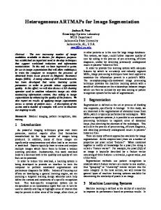
The algorithm needs to handle easily all possible fusions in a given partition. For an efficient implementation, the representation of the data has to be designed carefully. We have chosen a graph representation : the tiles of the partition are the nodes ; two nodes are linked by an edge if the corresponding regions are neighbors ; the valuation of the edge represents the similarity measure between both regions. Figure 1 presents a partition with 5 flat regions, represented first as an image and then as a neighborhood graph.

II.1.

Description of the region merging algorithm.

The region merging algorithm [8] is an iterative process. At each iteration we obtain a new partition in which the two most similar adjacent regions have been merged. Thus we obtain a series of partitions that describe the image with a decreasing degree of precision and at the same time with a more synthetic information. Let us describe the process in more detail. Let P0 be an initial partition (for example the set of flat-zones of an original image) with No regions : Po,1, P o , 2 , ' " ' , PO,No. The region merging algorithm builds a series of partitions P 0 , / ~ Pi, P i + I , " ' " , Pn ; Pi is the partition obtained after i steps of fusion. In order to obtain Pi+l from Pi we merge the two most similar regions of Pi, for example Pi,j, Pi,k, and we obtain the region Pi+l,t of the partition P,i+I (Pi+l,l = Pi,j U Pi,k). Thus Pi+l has one region less than P~. So, if Ni is the number of regions of Pi, we have Ni = No - i. As the fusion process goes on, the partition gets coarser and coarser. It follows from the fusion mechanism that the regions of a partition Pi are the union of a certain number of regions of P0. Hence the union of all partitions which are created by successive fusions is a partition tree, amenable to rate optimisation techniques described in [4]. The region merging algorithm processes an image, not pixel by pixel, but flat-zone by flat-zone. Thus it is a connected operator. This segmentation technique has two major advantages : - - the merging of flat zones removes existing contours but never generates new ones. This feature garanties that the shape of the objects is preserved; - - after a certain number of fusions, based on simple criteria such as contrast, more complex attributes may be ANN. TI~LI~COMMUN.,52, n ~ 7-8, 1997

procedure region_merging { E v a l u a t e t h e s i m i l a r i t y between regions o f e v e r y couple of adjacent regions ; s t o p = v e r i f y if s t o p c r i t e r i o n i s r e a c h e d ; while { ! stop) { (P_ij, P_ik} = f i n d t h e c o u p l e o f m o s t similar adjacent regions ; merge (P_ij, P_ik) ; Update the valuation of the new neighborhood relations ; s t o p = v e r i f y if s t o p c r i t e r i o n i s r e a c h e d ; }/* e n d w h i l e *I } I* e n d _ p r o c e d u r e *I

FIG. 1. - - Images and graphs. (a) input image ; (b) associated graph. Images et graphes. (a) image d'entrde , (b) graphe associd.

At each fusion step, the edge of lowest valuation will be the first edge to be removed because it separates the two most similar regions. For this reason, it is important to have an easy access to the edge with the lowest valuation. Hierarchical queues [5] precisely permit an easy retrieval of data, ranked according increasing orders of their numerical value. These queues accept the data in any order. The extraction of items out of the hierarchical queue obeys two levels of prioriy : 1) high priority items are extracted before lower priority items; 2) among all 2/11

399

B. MARCOTEGUI. -- BOTTOM-UP SEGMENTATION OF IMAGE SEQUENCES FOR CODING

items with the same priority, the item who entered the queue first is extracted first. Applied to the partition until convergence, the present algorithm will necessarily end up with a partition with only one region. It does not make sense to go so far. A stopping criterion has to be build in the algorithm. This criterion depends of course of the target of the segmentation. If the target is a unique partition, then one of the following criteria may be applied : a target number of output regions, a target number of output contour points, a compression rate (a combination of the number of regions and of the number of contour points), or any other functional which has to reach its minimum or maximum. If the target is creating a partition tree, then the desired coarsest partition has to be defined with the same criteria as above. The output will be the complete tree. For further treatment, a coarser subtree may be extracted from the complete tree for further processing. For instance the rate distortion techniques described in [4] would be relatively slow if the structure of the tree possesses too many levels.

II.2. Importance of how re-evaluating the edges after each fusion. The region merging algorithm makes structures crystallize : as similar regions merge, larger and larger homogeneous regions appear. At a first glance, this principle of image segmentation seems appealing and should lead to good image simplifications. The result however is largely disappointing. Let us analyse the results obtained by a blunt application of this method to real images, as we have done on the original image of foreman in 3(a). The result is presented in 3(b) and is surprisingly bad : a high number of meaningless small regions are present among some large regions, which have eaten up practically everything of interest in the image. Why is the result so bad ? The answer may be found by analysing the following simple situation. Imagine we have three regions A, B, C (see Fig. 2). We give a valuation to each frontier (A-B, A-C, B-C) and we remove the frontier of lowest valuation (for example A-B). After this

relnoved frontier

A C

B

A

!B

NEW

I

C

VALUATION

FIG. 2. - - R e - e v a l u a t i o n a f t e r e a c h fusion.

Rgdvaluation aprbs chaque fusion.

fusion, regions A and B become a unique region A-B with one neighbor region C. But which similarity measure should be assigned to the edge between the region A-B and C ? The solution adopted in example 3(b) is to take the min value all along the new frontier (composed by two initial frontiers A-B and B-C :

valuation(A-B, C) = rain[valuation(A, C), valuation(B, C)]. This solution has been inspired by the watershed : the flooding progress by the lowest pass. But it leads to very bad results. The similarity of both regions A-B and C is not faithfully estimated by the preceding rule. Regions A and C may be relatively similar, but the region A-B seen as a whole may be much more dissimilar from C. In this case, the preceding rule would allow the fusion of A-B with C. As a matter of fact, if the strength of a long contour is equal to the strength of its weakest part, then its strength can only decrease with its length. This is the reason why very large regions have been created in the example of Fig. 3(b). At the same time, tiny regions without meaning are able to resist against any fusion 9 being small, in their contour there is less likely a weak part. In a general case we need to go back to the image and re-evaluate the similarity between the merged region and its neighbors. Nevertheless shortcuts are possible in particular situations. For example, if the merging criteria is the contrast, the new valuation may be estimated from the information of the graph, without coming back to the image. The new mean gray level of region A-B would be"

FIG. 3. - - C o m p a r i s o n o f d i f f e r e n t r e - e v a l u a t i o n m e t h o d s . (a) i n p u t i m a g e ; (b) r e - e v a l u a t i o n : m i v v a l u e ; (c) re-evaLuation : b a s e d on the w h o l e n e w r e g i o n .

Comparaison de diff~rentes mdthodes de rddvaluation. (a) image d'entrde ; (b) rddvaluation basde sur la valeur minimale ; (c) rdgvaluation basde sur la totalit~ de la nouvelle rdgion. 3/11

ANN. TI~LI2COMMUN.,52, n ~ 7-8, 1997

400

B. MARCOTEGUI. -- BOTTOM-UP SEGMENTATION OF IMAGE SEQUENCES FOR CODING

mean(A-B) mean(A) x Area(A) + mean(B) x Area(B) Area(A) + Area(B) and this mean gray level is used to re-evaluate the contrast of region A-B with its neighbors. The result obtained with this re-evaluation is shown in Figure 3(c). The comparison between both methods shows that re-evaluations based on the whole new region outperforms that of a rain value of initial valuations. This example illustrates the fundamental importance of how re-evaluating frontiers as the fusions go on. The strength of a frontier can be evaluated with more and more accuracy as the frontier becomes longer and the adjacent regions bigger.

11.3.

Pre-processing.

The preceding section has shown how important is the method for re-evaluating the edges of any new region created by fusion of two adjacent regions. A careful analysis of the result will show that another preprocessing step will be needed. The partition of Figure 3(c) has 550 regions. But among them, 422 regions (76%) are isolated pixels. Figure 4 shows that most of them are located in areas of sharp transition between homogeneous regions. These isolated points are indeed not significant regions. Why does the algorithm tend to preserve those regions ? An explanation can be found when analysing the gray-tone distribution along a line of the image. Figure 5 shows the gray level function of line 59.

FIG. 4 . - -

R e - e v a l u a t i o n after each fusion.

Rddvaluation aprks chaque fusion.

FIG. 5. - - Profile of line 59 extracted from the original image. (a) original i m a g e ; (b) gray level of line 59 of original image.

Profil de la ligne 59 extraite de l'image d'origine. (a) image d'origine ; (b) niveau de gris de la ligne 59 de l 'image d'origine.

right neighbors have respectively the gray level values of 101 and 194. It is a sharp transition, the opposite case of the previous point. In these conditions the region merging algorithm tends to merge important regions (merging step by step the smooth local transitions) and to preserve non significant regions such as those corresponding to noise or to sharp transitions. This is why a pre-processing has proved to be necessary. Its goal is to remove all useless regions which are still preserved by the current algorithm : -noise, and -the transition zones. 11.3.1.

Elimination

of noise.

Connected filters are ideal for this purpose, since they remove noise while preserving the shape of the remaining objects. More precisely we use an alternated area filter (area opening followed by an area closing) of t0 pixels for a QCIF image (176 x 144 pixels). This filter reduces the number of flat-zones of the image (the flat-zones grow) while the visual aspect remains close to the original. The alternated area filter ensures that the extrema of the image (the maxima and the minima) have an area equal to or bigger than a given threshold. This filter mostly removes the noise but it does not affect the transition zones; the steps going from an extremum to another one are not modified, even if they are small. The next section explains how to eliminate such transition zones.

This gray-tone profile shows the following : - - the white bands of the building, that look homogeneous present in fact gray level oscillations due to noise. Around pixels 35 and 120 we have other examples of noise ; - - the left eyebrow (structure extended from pixels 70 to 90) is represented by a valley formed by steps of small amplitude, in other words, it is made up of smooth local transitions ; -let us now consider the transition around pixel 126. Pixel 126 has a gray level of 152 and its left and ANN. TI;;LECOMMUN., 52, n ~ 7-8, 1997

11.3.2.

Elimination

of the transition

zones.

Transition zones are small tim-zones with both higher and lower neighbors. They fool the correct estimation of the similarity between larger adjacent regions in two opposite ways : - - in some cases they provide a path of smooth transitions and facilitate the fusion of two larger regions which should remain separated; - - in other cases they are present within a sharp transition zone between two larger regions. In this case, 4/I 1

401

B. MARCOTEGUI. -- BOTTOM-UP SEGMENTATION OF IMAGE SEQUENCES FOR CODING

they present a sharp contrast with both their higher and lower neighbor; hence they resist against any fusion and the necessity to code them spoils bits. For eliminating such noisy transition zones, we will use the result of the area filter. The area filter does not modify the transition zones but helps us to locate them. As shown in [1] the extrema of an image are regions with an important visual meaning. After an area opening and an area closing of a given size, all extrema of the image will have a size larger than the size of the filters. Hence, every region smaller than the filter size may be considered as a transition region between two extrema. Nevertheless an image may have significant stairs. This is why we have retained as transition zones all regions with a size bigger than half the filter size used for the detection of extrema. In that way the resulting partition (without transition zones) preserves the visual details and does not have isolated pixels. Once the transition zones have been located, they are removed, leaving holes in the partition. These holes are filled using a region growing algorithm applied on a flat zone level : the transition zones are assigned to a bigger neighbor, following a contrast criterion. Figure 6 illustrates the intermediate stages of the preprocessing. The original image (Fig. 6(a)) is in QClF format (176 x 144 pixels) and has 19 342 flat-zones. The area filter of size 10 reduces the number of flatzones to 11 171, and preserves the visual aspect (Fig. 6). Among these 11 171 flat-zones only 735 are bigger than 5 pixels (the half of the filter size). These flat-zones (in white in Figure 6(c)) are considered as markers in a region growing procedure and the transition zones (in black in Figure 6(c)) are assigned to a neighbor marker. The result is an image with 735 regions (Fig. 6(d)).

This preprocessing stage has indeed greatly reduced the number of regions without significantly modifying the visual aspect of the images; it has the following advantages for the subsequent region merging stage : - - the searching of homogeneous regions becomes simpler, - - the merging process becomes faster : instead of having 82 474 frontiers in the original image (51 114 in the filtered image) that we have to evaluate, sort and manage, we have only 4 060 frontiers. II.3.3.

Smoothing the contour.

The removed transition zones are assigned to their most similar neighbor. Without special care, this procedure will produce irregular contours, which are costly to code. Figure 7 illustrates the problem. Image 7(a) contains two main regions (M1 and Mz) and one transition region (R). The contrast R - M1 is C1 = 51 while the contrast R - M2 is (72 = 49. Considering only the contrast criterion, R will be assigned to the marker M2 (see Fig. 7(b)) because the contrast Cz is lower than C1.

FIG. 7. - - Region growing without and with contour smoothing. (a) original image ; (b) region growing : contrast ; (c) region growing : contrast + smooth contour.

Croissance de rdgion sans et avec lissage de contour. (a) image d'origine ; (b) croissance de rdgion basde sur le contraste ; (c) croissance de rdgion basde sur le contraste et le lissage.

However, the difference between C1 and C2 is small and meaningless; in this case it would be better to chose the least expensive solution from a coding point of vue and to assign R to M1 (see Fig. 7(c)). In [9] the similitude between one pixel p and one marker Mi is defined as a weighted sum of a contrast term based on the gray-tone information, and a contour complexity term : (1)

FIG. 6. - - Stages of the pre-processing. (a) original image ; (b) filtered image ; (c) flat-zones bigger than the half of the filter size ; (d) partition with 735 regions.

Etapes de prdtraitement. (a) image d' origine ; (b) image filtrde , (c) zones uniformes plus grandes que la moitid de la mille du filtre ; (d) partition en 735 rdgions. 5/11

similitude(p, Mi) = a • contrast(p, Mi)+ (1 - a) x contour complexity(p, Mi).

The contour complexity is defined as the number of contour points added to the contour of Mi if the pixel p is assigned to Mi ; in other terms it is the number of neighboring pixels of p that do not already belong to the marker Mi. Note that the total similitude measure is decreasing with the contrast between pixel and marker : the more similar the pixel is to the marker, the closer the similitude to zero. The parameter a allows to give more or less importance to the contour (compared to the contrast). When a is small, the contours are smoother, ANN. TELI~COMMUN.,52, n ~ 7-8, 1997

402

B. MARCOTEGUI. -- BOTTOM-UP SEGMENTATION OF IMAGE SEQUENCES FOR CODING

but the segmentation, being not sufficiently driven by the gray-tone content of the image, may lose in quality. We have followed the same line of thought, but adapted it to our context of flat zones manipulation. Suppose we want to define the contour complexity term contour-complexity(R,Mi) associated to the merging of a region R to a marker Mi. It will be the difference between the contour lengths after and before the fusion of the region R with the marker Mii. It is easy to see that it is equal to the difference between the external contour (number of neighboring pixels of R that do not belong to Mi) and the common contour R - Mi (number of neighboring pixels of R belonging to Mi). This criterion favors the merging of regions in a longitudinal way (region R in Figure 8) rather than regions added in a transversal way (region/~' in Figure 8).

i

:

FIG. 9. - - S m o o t h i n g c o n t o u r . (a) r e g i o n g r o w i n g : c o n t r a s t ; (b) r e g i o n g r o w i n g : c o n t r a s t + s m o o t h i n g c o n t o u r ; (c) 13 5 9 3 c o n t o u r points ; (d) 11 8 6 2 c o n t o u r points.

A

Lissage des contours. (a) croissance de rdgion basde sur le contraste ; (b) croissance de rggion basde sur le contraste et le lissage ; (c) 13 593points de contour ; (d) 11 862points de contour.

Mi

Acontour

=

Ie

-

1i

FIG. 8. - - M e a s u r e o f c o n t o u r i n c r e a s i n g .

Mesure de la croissance du contour.

Using this criterion we have obtained the image of Figure 9. If we compare with the previous result we realize that with the same number of regions we have 11 862 contour points instead of 13 593.

III.

the coding capabilities which are at hand : two regions will be considered to have a similar texture, when the coder is able to represent the union of both regions with a unique texture model without introducing an unbearable distortion. We also learned how important it is to re-evaluate the similarity relations between each newly created region with its neighboring regions. Hence this re-evaluation will be systematically applied in the sequel.

M E R G I N G CRITERIA III.1.

Let us summarize what we have learned so far. The connected filters applied to the initial image reduce significantly the number of regions but leave a high number of spurious transition regions. We have presented an algorithm for eliminating these regions. This leaves us with a clean partition containing an oversegmentation with a reasonable number of regions and smooth contours. Our goal will now be to reduce this oversegmentation in order to obtain candidate regions which are suitable for coding. We will present successively various merging criteria which will govern the fusion of regions. For the first fusions, simple criteria are used. As the regions become bigger, more complex similarity relations may be faithfully estimated on neighboring regions and the criteria become more complex : for instance similarity of texture or of motion. In particular, we will by then be in the position to explicitely introduce ANN. TI~LE,COMMUN., 52, n ~ 7-8, 1997

Contrast criterion.

This criterion evaluates the strength of a frontier as the absolute difference between the mean gray levels of two adjacent regions. After each fusion we calculate the new gray level average of the new region and we re-evaluate the strength of its frontiers. Applying this algorithm to the result of the pre-processing stage and taking as stopping criterion 5000 contour points of the output segmentation we obtain the image of Figure 10. The partition has 101 regions and we can observe that the obtained regions seem to be perceptually significant. Nevertheless, this criterion generates sometimes false contours, that means, contours that do not correspond to frontiers which are visually significant. It happens in presence of progressive gray level variations. We have an example of this default in the left white triangle of the building. In order to avoid this problem we have developed a local contrast criterion. 6/11

403

B. MARCOTEGUI. -- BOTTOM-UP SEGMENTATION OF IMAGE SEQUENCES FOR CODING

Applying the region merging algorithm with this criterion to the result of the pre-processing stage we obtain the image of Figure 12. As shown by the result, we have avoided the problems caused by the contrast criteria : the resulting regions correspond better to the objects present in the scene.

FIG. 10. - - Segmentationobtainedusing region merging algorithm with contrast criterion. Segmentation obtenue en utilisant un algorithme de fusion de rggions selon un critbre de contraste.

III.2.

Local contrast criterion.

After a first stage of fusions based on the difference of gray level average of adjacent regions we base the next stage of fusions on the local contrast. This measure will avoid false contours while keeping frontiers which appear as significant for the eye. We compute the local contrast in the following way : for each couple of regions (R1, R2) we compute the gray level average not in the whole region as beforehand but on a band of thickness e along the frontier (see Figure 11). Thus we obtain NI and N2. The local contrast is given by the absolute difference between N1 and N2.

Lo=m Cont,ast(R I, ~

R1 1

) : I N I - r~l

R2

I fmntier(Rt, R~)

FIG. 11. - - Re-evaluationafter each fusion.

Rddvaluation aprks chaquefusion. After each fusion the frontiers of the new region must be re-evaluated with the new local contrast. This new valuation is given by the formula : (2)

new valuation = E i Nlili

• i N2ili

where i correspond to each component of the new frontier, li the initial length of component i and Nli and N2i the gray level average of each side of the frontier. For simplicity reasons we have computed the weighted sum of the previous local contrast measures along the new frontier : (3)

new valuation - ~-~i vil~,

where vi is the initial valuation of the ith component. 7/11

FIG. 12. - - Segmentation obtained using region merging algorithm with local contrast criterion. (a) partition with 99 regions ; (b) contours of image (a). Segmentation obtenue en utilisant un algorithme de fusion de rggions selon un critkre de contraste. (a) partition en 99 rggions ; (b) contours de l'image (a).

III.3.

Texture criterion.

Let us not forget that the segmentation is not an aim in itself. We segment the image in order to find a partition for which we will have to code the contours of the tiles and the texture for each tile. The partition will be optimal if it yields the best image representation after coding for a given coding cost. For this reason, the texture coding capabilities of the coder have to be taken into account already at the very stage of the segmentation. The idea is to merge the regions that are satisfactorily represented together. The gain in coding cost comes from the fact that : - - only one set of texture parameters is used to describe the resulting merged region, - - contour pixels (which must be coded) disappear in the merging process. Thus, the coding cost is reduced while the visual quality is not significantly affected. To do so, we need a measure for the texture resemblance in adjacent regions. 111.3.1. Texture regions.

resemblance

measures

of

adjacent

Resemblance of texture parameters : the fastest similarity measure between the textures of adjacent regions would be based on the comparison of the texture parameters themselves. This is however not feasible for most texture coding techniques, because the parameters have a complex behaviour and dynamics. For instance the texture representation by orthogonal polynomials proposed in [2] represents the polynomials in a reference space depending upon the shape of the region. For two adjacent regions, these reference spaces have nothing in ANN. Tt~LI~COMMUN.,52, n~7-8, 1997

404

B. MARCOTEGUI. -- BOTTOM-UP SEGMENTATION OF IMAGE SEQUENCES FOR CODING

common. For this reason, we will have to resort to a more complex technique, where the texture in adjacent regions and in the union will have to be computed really. Loss of quality caused by a fusion : when two regions merge, only one texture model (instead of one by region) represents the union of them. This may lead to a loss of quality (not necessarily so, if the model for the union is more complex than the models used for each region separately). If we merge only regions for which this loss of quality is the smallest possible, we obtain a segmentation optimized from the point of view of the quality of its regions. The problem of this measure is that it is based on a relative criterion. The same loss of quality is allowed for regions of initial good quality as well as for those whose initial quality was poor. The result is an image of inhomogeneous quality in which defects are accentuated. In order to avoid this defect, we will have to define an absolute criterion rather than a relative criterion. Quality of adjacent regions after fusion " this measure is based on the quality of the texture coding after fusion. In contrast with the previous measure, it produces images of homogeneous quality, which leads to better visual aspects. This is the criterion we are going to use in the following. The quality estimation after a fusion is not computed on the resulting merged region. Quality is independently estimated in each of both regions and the minimum of both quality measures is considered. Otherwise, small regions could be extremely badly represented after fusion : this is due to the fact that their contribution to the total error would be negligible. The result obtained by the local contrast can be simplified using the texture criterion. Thus if we merge all the regions keeping a quality bigger than 30 dB after fusion based on texture similarity, we reduce the number of regions from 99 (Fig. 13(a)) to 61 (Fig. 13(c)) without deteriorating the visual quality (from 32.15 dB (Fig. 13(b)) to 31.10 dB (Fig. 13(d))).

IV.

IMAGE SEQUENCES SEGMENTATION

IV.1. Time-stability and inclusion of new regions : region merging algorithm with markers. IV.I.1. bility.

The right balance between time stability and flexi-

Since we have solved the problem of segmenting a still image, we may think that the problem of segmenting a sequence is solved as well : one could treat each new frame in a sequence as an intra image and segment it independently of the past. This would of course lead to catastrophic results, in coding cost but also in coding quality. Segmentation is an unstable process. In spite of the visual similarity between two adjacent frames, ANN. T~LI~COMMUN., 52, n ~ 7-8, 1997

FIG. 13. - - R e g i o n m e r g i n g algorithm based on texture criterion. (a) partition with 99 regions ; (b) coded i m a g e from (a), 32.15 dB ; (c) partition with 47 regions ; (d) coded i m a g e from (c), 31.10 dB.

Algorithme de fusion de rdgions selon un critOre de texture. (a) image codde correspondante : qualitd 32,15 dB ; (b) partition en 47 rYgions ; (c) image cod(e correspondante : qualitd 31,10 dB.

their segmentations obtained independently will be quite different; the least gray-tone fluctuation would favour different region fusions. Thus, any correspondence between tiles of two successive segmented images would be almost suppressed. For this reason the coding cost would be maximal for motion, contours and texture. Most regions would be treated in intra mode. Furthermore the visual quality of the coded sequence would be bad : the contour fluctuation and the texture model fluctuations from image to image would be clearly visible. In order to exploit fully the temporal redundancy of image sequences and obtain a good quality of the coded sequence, one has to resort to a technique which garanties a good temporal stability of the segmentation. On the other hand, sufficient flexibility should be present as well, otherwise it would be impossible for a new object appearing in a frame to be introduced into the segmentation. Finding the right balance between time stability and flexibility is the real challenge for the segmentation of sequences : - - time stability reduces the coding cost : it allows the prediction of the current frame from the previous frame, - - the inclusion of new regions and the disparition of vanishing regions is necessary in order to follow correctly the evolution of the scene. IV.1.2. Hard projection : time stability and flexibility are treated in successive order.

The approach presented in [10] works in two steps : - - the first step cares uniquely for time stability : the tiles of the current segmented image serve as markers for the segmentation of the next image. This forbids the 8111

405

B. MARCOTEGUI. -- BOTTOM-UP SEGMENTATION OF IMAGE SEQUENCES FOR CODING

apparition of any new region which does not correspond to a marker in the preceding image. We will call this step

hard projection ; - - the second step cares for the introduction of new regions. The projected image is coded, i.e. the tiles of the mosaic image are dressed with texture. The coded image is then subtracted from the true image producing a residue image. The new regions will appear in the residue image as a strong positive or negative signal. The regions which were correctly predicted by the projection step produce a zero or a weak signal. However, there are also imperfections in the projection itself or in its coding. These imperfections also will produce a signal in the residue image. A specific marker extraction algorithm produces a new set of markers enabling to resegment the projected image, in order to introduce new regions and to correct the projection errors. Good results have been obtained by this two step technique. The method also has some drawbacks. The projection step assigns all pixels of the new frame to segmented regions of the previous frame. Imagine that A and B are two regions of the previous frame and that a new region C appears in the forefront of the image covering partially regions A and B. The projection step will share out region C between regions A and B. This creates a meaningless contour within the region C in the projected image : the contour is meaningless because it ought to be absent in the final segmented image. The introduction of new regions however does simply resegment the projected partition and preserves the meaningless contour. A third step is then necessary, which examines whether some fusions are possible among the newly introduced regions. Analysing correctly the residue image in order to construct the markers for the new regions is another delicate part of this approach : as a matter of fact the residue of the projected partition contains not only the new regions but also the coding errors. Searching new regions in the residue is more difficult than in the original image.

This restrictive merging rules forbid the apparition of any new regions. In order to let new regions appear, we have to loosen the merging rules. Too loose rules would damage time stability if they allow two regions containing different markers of the previous segmentation to fuse. The good compromise between time stability and flexibility is obtained if all fusions are allowed except the fusion of a marker with another marker; this remaining prohibition garanties a sufficient time stability, whereas the allowed fusions permit both the projection and the emergence of non marked regions (new regions). In order to segment an image sequence we use a region merging algorithm taking as markers the regions of the previous segmentation. The results of this procedure are the following : - - regions of frame t - 1 are projected into frame t (by fusions of regions t - 1 with regions t), - - new regions may spontaneously appear by independent crystallization in the current time (fusions of regions t), without an external marker selection. The following Table I summarizes the behavior o f hard projection and soft projection : TABLE I. - - Behavior of region growing algorithm and region merging algorithm with markers.

Comportement de l'algorithme de croissance de rdgions et de l'algorithme de fusion de rggions avec marqueurs. hard projection

soft projection

marker with non-marker

allowed fusion

allowed fusion

non-marker with non-marker

forbidden fusion

allowed fusion

marker with marker

forbidden fusion

forbidden fusion

When a non marker fuses with a marker, the whole region becomes a marker. On the other hand, when a non marker fuses with another non marker the union is still a non marker (so its fusion with a marker is still allowed).

IV.1.3. Soft projection : a one step approach dealing with stability and flexibility at the same time.

IV.2.

We propose here an approach where new regions are introduced already during the projection phase; the method being based on a relaxation of the methods used for hard projection, we will call this method soft projection. The region merging algorithm is applied to the same sliding window as in [10]. The sliding window contains the previous segmentation (whose regions play the role of markers) and the new image to code (the construction of this sliding window implies a motion compensation stage in order to maximise the correspondence between both images). The construction mechanism has been explained in detail in [6]. Expressed in terms of fusions of regions, pure projection means that a region of the current image can only merge with a marker of the previous segmentation.

The coding of an image in inter mode is made in two steps : - - description of the current image by motion compensating the preceding image. If, as in our case, the description of the image is region based, this motion compensation has to be made region by region. Thus part of the information to be transmitted consist in motion vectors for each region of the previous partition; - - coding the error : the preceding step is unable to accurately predict the current image. This may be due to the appearance of new regions or to the inadequation of the motion model which is used. In this case the prediction error has to be coded. This coding scheme relying on a motion model for each region offers the possibility of new fusions of

9/1 l

Motion criterion.

ANN. TI~LI~COMMUN.,52, n ~ 7-8, 1997

406

B. MARCOTEGUI. -- BOTTOM-UP SEGMENTATION OF IMAGE SEQUENCES FOR CODING

adjacent regions : if several regions have a coherent motion (which is frequently the case), they can be correctly compensated together. Such a fusion based on motion similarity reduces significantly the coding cost (less contour pixels, less motion vectors and less parameters of texture correction). Figure 14 illustrates this idea.

time = t-p

Q= max(Qt,Q2) .AL

Qt = min( Ql ,Q~ ) i

Q2 = min( Q~ ,Q~ ) /

Q~

Q~"

\

Q~

Q~

time = t FIG. 15. I Suboptimal computation of the compensation quality after fusion.

Calcul sous-optimal de la qualitd de la compensation aprks fusion.

Without motion fusions

With motion fusions FIG. 14. I

Goal of motion criterion.

But de crit&e de mouvement.

To implement this criterion we have to define a resemblance measure between motion of adjacent regions. We use the same type of solution as for the texture criterion : we base the similarity measure between two regions A and B on the quality of the compensation of the union A U B. The motion model of the region A U B is separately applied to both regions A and B. The lowest quality obtained on A or B is taken as the measure of similarity. As we explained it already in the case of the texture similarity criterion, this rule allows to avoid that small regions are completely dominated by larger regions. Due to the fact that the computation of a motion vector for each couple of adjacent regions leads to an expensive algorithm in terms of computational time, we have implemented a suboptimal algorithm. Instead of calculating a motion vector for a couple of regions, we consider -5-~1 (motion vector of R1) and 7 2 (motion vector of R2) as two approximations of --~ (motion vector of R1 U R2) and we choose between them the one that leads to a better compensation quality. Figure 15 illustrates this procedure. An example of motion based merging is presented in Figure 16. Figures 16(a) and (b) show the two original images. Using backward motion estimation of [3] with the segmentation of Figure 16(c) (89 regions) we obtain the image of Figure 16(d). The quality of this compensation is 28.5 dB. Merging those regions that can be compensated together we obtain the segmentation of the Figure 16(e) (35 regions). The resulting compensated image is presented in Figure 16(f). Its quality is 26.7 dB. ANN, TI~LI~COMMUN.,52, n ~ 7-8, 1997

FIG. 16. - - Motion simplification. (a) original image 1 ; (b) original image 2 ; (c) segmentation of (b) with 89 regions and 4 988 contour points ; (d) image (a) compensated with respect to (b) from the regions of image (c) ; (e) regions of homogeneous motion obtained by motion fusions from image (c). 36 regions and 2 951 contour points ; (f) image (a) compensated with respect to (b) from the regions of image (e).

Simplification du mouvement. (a) image d'origine 1 ; (b) image d'origine 2 ; (c) segmentation de (b) en 89 r~gions et 4 988 points de contour ; (d) image (a) compens~e par rapport it (b) a partir des rdgions de (c) ; (e) r~gions de mouvement homogbne obtenues par des fusions du mouvement de l'image (c) 36 rdgions et 2 951 points de contours ; (f) image (a) compensde par rapport gt (b) b partir des r~gions de (e). 10/11

B. MARCOTEGUI. - BOTTOM-UP SEGMENTATION OF IMAGE SEQUENCES FOR CODING

Obviously the fusion of adjacent regions based on motion is a source of economy : one motion model has to be used instead of two, and the common boundary between both regions does not need to be coded. On the other hand, the coder has to inform the receiver about the fusions which occurred in the previous partition, meaning additional bits to spend.

IV.3. Integration of the motion fusion in the complete architecture.

The fusions based on motion improve the coding efficiency but unfortunately they disturb the earlier stages of segmentation based on texture similarity. The segmentation stage uses a recursive approach : the regions of the previous segmented frame are the markers of the current time. But the fusion based on motion criteria generally produces regions which are not homogeneous anymore in texture. For this reason the texture fusion algorithms which we have presented earlier will fail : the mean gray level or the texture parameters of these regions are not representative and so we can not compare those regions with the current frame. After motion fusion, the new regions are not anymore a reliable set of markers for texture fusion with the next frame. In order to solve this problem we propose to work at two resolution levels : - - a fine segmentation level that contains texture homogeneous regions. This level is used for the texture fusion stages but nor for coding; - - a coarse segmentation level that contains motion homogeneous regions. The fine segmentation is used by the transmiter to help the projection of the previous regions. The coarse segmentation is sent to the receiver allowing the reduction of the coding cost. The regions of the coarse segmentation are a union of one or several fine segmented regions.

V.

CONCLUSION

In the context of coding, segmentation has to be revisited. Depending upon the coding techniques, the

11/11

407

segmentation will not be the same. A more powerful texture coding method will allow to represent a part of an image as a unique region where a less sophisticated technique would require several regions. The same is true for motion models. The segmentation method we have presented in this paper permits this feedback between segmentation and coding. The fusion of regions is based on criteria of increasing complexity. First simple connected filters, then criteria based on more meaningful and coding depending features : the ability of two regions to be coded as a unique region, whatever the coding technique. Finally, the soft projection method ensures a good temporal stability of the resulting segmentation, and at the same time enough flexibility for accepting any new object appearing in the scene. Iterative fusions of regions naturally build a segmentation tree, amenable to sophisticated optimal or to fast suboptimal selection algorithms, able to extract the best partition out of the tree [4].

Manuscrit refu le 20 mai 1997.

REFERENCES

[1] CRESPO (J.). Morphological connected filters and intra-region smoothing for image segmentation. PhD Thesis, School of Electrical Engineering, Georgia Institute of Technology (1993). [2] GILGE (M.), ENGELHARDT(T.), MEHLAN (R.). Coding of arbitrarily shaped image segments based on a generalized orthogonal transform. Image Communication (1989), 1, n~ 2. [3] LEE First results of motion prediction based on a differential estimation method. In SIM(94) 35 COST 211, Tampere (June 1994). [4] MARCOTEGUI (B.), MARQUI~S (E), MORROS (R.), PARDAS (M.), SALEMBIER (P.), Segmentation of video sequences and rate control. Ann. Tgldcommunic. (1997), 52, n~ 7-8, pp. 380-388. [5] MEYER (E). Algorithmes ~t base de files d'attente hi@archique. Technical Report NT-46/90/MM, Ecole des Mines de Paris, Centre de Morphologie Mathgmatique (Sep. 1990). [6] MEYER(E), MARQUI~S(E). Segmentation in object based coding : general requirements. Ann. Tglgcommunic. (1998) (h parai'tre). [7] MEYER (E), OLIVERAS(A.), SALEMBIER(E), VACHIER(C.). Morphological tools for segmentation : connected filters and watersheds. Ann. Tgl(communic. (1997), 52, n~ 7-8, pp. 367-379. [8] MONGA (O.). Segmentation d'images par croissance fii6rarchique de r6gions. PhD Thesis, Universit6 Paris Sud, Centre d'Orsay (1988). [9] PARDAS (M.), SALEMBIER (P.). Time-recursive segmentation of image sequences. In EUS1PCO-94, Edinburgh (Sep. 1994). [10] PARDAS(M.), SALEMBIER(P.). Segmentation of video sequences for partition tree generation. Ann. Tilgcommunic. (1997), 52, n ~ 7-8, pp. 389-398.

ANN. TI~LI~COMMUN.,52, n ~ 7-8, 1997