AUGUST 1997
1031
TIRABASSI AND RIZZA
Boundary Layer Parameterization for a Non-Gaussian Puff Model T. TIRABASSI Institute FISBAT of CNR, Bologna, Italy
U. RIZZA Institute ISIAtA of CNR, Lecce, Italy (Manuscript received 22 March 1996, in final form 10 June 1996) ABSTRACT The paper presents two boundary layer parameterizations for a model based on a general technique for solving the K equation using the truncated Gram–Charlier expansion (type A) of the concentration field and a finite set of equations for the corresponding moments. The two parameterizations allow the model to be applied routinely using as input simple ground-level meteorological data acquired by an automatic network. A preliminary performance evaluation is shown in the case of continuous emission from an elevated source in a variable boundary layer (with a time resolution of 10 min).
1. Introduction
2. The model
A distorting effect of the variation with height on the mean wind, both in speed and direction, is often observed in the development of puffs or plume smoke. This effect is most prominent in stable stratified conditions. In fact, wind shear creates a variance in the wind direction, while vertical diffusion destroys this variance and tries to reestablish a nonskewed distribution. The interaction between vertical mixing and velocity shear is continuously effective. In order to take into account the above phenomenon, we developed a model for the dispersion of passive non-Gaussian puffs. The model is based on a general technique for solving the K equation using the truncated Gram–Charlier expansion of the concentration field and the finite set of equations for the corresponding moments. Actually, the Gram–Charlier expansion of type A is a classic method for approximating a given distribution with moments of any order, basically consisting of a truncated expansion in terms of Hermite functions, whose coefficients are chosen so as to reproduce the sequence of moments of the distribution up to a given order. In particular, the model is well suited to applications where interest is focused mainly on certain overall properties of the horizontal patterns, rather than on specific values at particular point receptors.
The advection diffusion equation describing the time evolution of concentration C, due to a release at time t 5 0 of a quantity Q of passive material by an elevated source placed at (0, 0, 1), in a horizontally homogeneous atmospheric boundary layer is
Corresponding author address: Dr. Tiziano Tirabassi, Institute FISBAT of CNR, Via P. Gobetti 101, I-40129 Bologna, Italy. E-mail:
[email protected]
q 1997 American Meteorological Society
1
2
]C ]C ]C ] ] 1 ]2C ]2C 1u 1 dy 5 Kz C 1 Kh 2 2 1 2 ]t ]x ]y ]z ]z d ]x ]y 1 d(t)d(x)d(y)d(z 2 1),
(1)
where x is the along-wind coordinate, y the crosswind one, and z the height; d means delta function; (u, y, 0) is the wind velocity vector; and Kz and Kh are the eddy diffusivities for vertical and horizontal turbulent transport, respectively. All variables are nondimensional, with the corresponding scale factors being given by H 2s /Ks for time, UsH 2s /Ks 5 dHs for a distance along the x axis, Hs for the height and distance along the y axis, Ks for diffusivities, us for wind speed, and Q0/(dH 3s ) for concentration. Here, K s and us represent the values of the dimensional u and K profiles at the dimensional source Hs. The initial condition is limC(x, y, z, t) 5 0,
t→01
and the no-flux boundary conditions applied at the ground level and at the mixing layer height (zi) are Kz
]C 50 ]z
for z 5 0 and z 5 z i .
Since C is exponentially small at asymptotic distances
1032
JOURNAL OF APPLIED METEOROLOGY
from the source on any horizontal plane, we can introduce the moments of its (x, y) distribution:
EE
`
C m, n 5
x m y n C dx dy,
(2)
j5
x2b , s
b5
C1 , C0
VOLUME 36
2`
where m and n are nonnegative integers. Of course, Cm,n are functions of height and of time. Their time evolution is governed by the double sequence of one-dimensional diffusion equations, equivalent to the single three-dimensional Eq. (1):
s2 5
C2 2 b2, C0
Sk 5
1 C3 2 3bs 2 2 b 3 , s 3 C0
Ku 5
1 C4 2 6b 2s 2 2 4bs 3 S k 2 b 4 . s 4 C0
1
2
and ]C0,0 5 DC0,0 1 d(t)d(z 2 1) ]t and ]C m, n 5 DC m, n 1 muC m21,n 1 ndy C m, n21 ]t 1 Kh
[
]
for m 1 n ± 0 and D, the differential operator (]/]z)Kz(]/ ]z). The initial condition is therefore written as limC m, n 5 0,
1
at z 5 0, z i .
sÏ2p
[
11
1 where
1
2
Ku 2 3 4 (j 2 6j 2 1 3) 24
]
Sk j (j 2 2 3) , 6
2
z K z 5 kw*z 1 2 , zi
A classic method for approximating a given distribution with moments of any order is the Gram–Chalier expansion of type A, which is basically constituted by a truncated expansion in terms of Hermite functions, whose coefficients are chosen so as to reproduce the sequence of moments of the function up to a given order (Kendall and Stuart 1977). In the case of one-variate function of the concentration C(x), truncated to the fourth order, if Sk is the skewness and Ku is the kurtosis, we have (Lupini and Tirabassi 1983) e2j 2/2
ku* z(1 2 z/z i ) 2 . F h (z/L)
(5)
During convective conditions (zi/L , 210), the friction velocity u* was replaced by the convective velocity w* as scaling velocity to give (Pleim and Chang 1992)
and the boundary conditions become
C ù C0
In order to evaluate the diffusion coefficients in Eq. (3), utilizing as input simple ground-level meteorological data acquired by an automatic network, we tested two different boundary layer parameterizations. We applied a parameterization proposed by Troen and Marth (1986), as presented in Pleim and Chang (1992). During near-neutral and stable conditions (zi/L $ 210), we adopted Kz 5
t→01
]C m,n 50 ]z
2
3. Boundary layer parameterization
1 m(m 2 1)C m22,n 1 n(n 2 1)C m, n22 d2 (3)
Kz
1
where the convective velocity is defined as w* 5 (bgw9u90 zi)1/3.
(7)
Here, bg is the bouyancy parameter and w9u90 the surface kinematics heat flux (w is vertical velocity and u the potential temperature). The prime indicates turbulent fluctuation variables. For the horizontal eddy diffusivity in unstable conditions, we use (Seinfeld 1986) Kh 5 0.1w*zi. In neutral stable conditions (Tangerman 1978), Kh 5 2KMz,
(4)
(6)
(8) (9)
where KMz is the maximum of Kz. The second parameterization used is based on Freeman’s work (Freeman 1977), in which vertical and horizontal eddy diffusivity coefficients Kz and Kh are derived from the Mellor–Yamada level 2 model (Mellor and Yamada 1974). In particular, we have
AUGUST 1997
1033
TIRABASSI AND RIZZA
[ [ [
TABLE 1. Friction velocity (m s21) for the different runs and time steps. Every time step corresponds to 10 min.
1 2 ]y ]z
2
K y 5 d K0 1 (2d9K M 2 K9)
Run
Time step
1
2
3
4
5
7
8
9
1 2 3 4 5 6 7 8 9 10 11 12
0.36 0.37 0.40 0.43 0.35 0.34 0.42 0.43 0.40 0.37 0.35 0.36
0.68 0.67 0.81 0.68 0.75 0.74 0.76 0.82 0.76 0.73 0.69 0.66
0.46 0.45 0.47 0.39 0.39 0.40 0.40 0.41 0.31 0.34 0.39 0.40
0.56 0.51 0.37 0.44 0.48 0.48 0.39 0.40 0.39 0.39 0.39 0.39
0.58 0.52 0.51 0.58 0.59 0.52 0.52 0.45 0.44 0.44 0.44 0.43
0.48 0.48 0.57 0.62 0.53 0.65 0.63 0.65 0.66 0.62 0.52 0.62
0.65 0.79 0.67 0.67 0.68 0.65 0.68 0.67 0.73 0.73 0.75 0.69
0.72 0.73 0.60 0.59 0.65 0.71 0.73 0.73 0.73 0.66 0.67 0.74
] 1 2] ] ]u ]z
2
K x 5 d K0 1 (2d9K M 2 K9) and
where
K9 5 a gd K0 5 q 2
(12)
,
(13)
]u (K 1 K H ) 2 K M , ]z M
13 2 L 2 2 1
2l1 1
0.6l1bg]u/]z KH , q
and KM is the turbulent viscosity defined by K M 5 a9(w 2 2 0.056q2 1 «w9u9 ), Kz 5 K H,
(10)
«5
where KH is the turbulent heat conductivity given by KH 5 Al2q.
(11)
d9 5
1 2 (6l1 /L1 ) , 1 1 6Bg9d]u/]z
B 5 1.6
d5
l1 2 1 , L2 9
3l2 , q
and g9 5
bgL2 . 2q
With strong convection, ] u/]z can change sign above the surface layer and remain slightly positive over most of the mixed layer. This implies negative KH values. In order to avoid such negative values, we used a modified flux gradient relation, as suggested by Deardoff (1972). The horizontal diffusion coefficients are
a9 5
d9 1 1 d9«]u/]z
and
Here, q is the turbulent kinetic energy and A5
2.1l 2bg , q 3l1 . q
(14)
Here, following Mellor and Yamada (1982), l1 5 0.92l, l2 5 0.74l, L1 5 16.6l, L2 5 10.1l, and l is the master length scale. All diffusion coefficients have been expressed in terms of vertical derivatives of the mean values of boundary layer variables and the turbulent kinetic energy. The relation of the kinetic energy to the mean field quantities is found by solving the algebraic equation (Freeman 1977), where s is the horizontal wind shear, s 2 K M 2 bgK H
]u q3 2 5 0, ]z L1
(15)
in which additional dependence on q is contained in KH and KM. This equation becomes a quadratic equation,
TABLE 2. Monin–Obukhov length (m) for the different runs and time steps. Every time step corresponds to 10 min. Run
Time step
1
2
3
4
5
7
8
9
1 2 3 4 5 6 7 8 9 10 11 12
226 223 283 242 236 242 247 238 283 221 232 229
2178 2227 2311 2160 2203 2286 2155 2228 2184 2389 2133 2375
2152 2194 2106 2101 2129 270 283 260 2106 242 2101 270
275 242 223 232 271 280 283 2101 2129 2129 2129 2129
2492 2215 2368 2735 2366 2273 2273 2262 2395 2395 2395 2759
271 280 264 2111 2177 267 287 271 256 2111 2215 2123
271 285 247 249 245 263 241 247 270 264 252 239
2793 2471 2202 2366 2633 213 588 2593 2471 2389 2375 2262 2252
1034
JOURNAL OF APPLIED METEOROLOGY
VOLUME 36
TABLE 3. Boundary layer height for the different runs. Run
zi (m)
1
2
3
4
5
7
8
9
1980
1920
1120
390
820
1850
810
2090
the coefficients of which depend on the mean quantities of the boundary layer through the gradient Richardson number Ri (Freeman 1977). Here, Ri has been evaluated following the relation Ri 5
Km R 5 a21 R f , Kh f
(16)
where a is from Yamada (1975) and the flux Richardson number Rf is evaluated with an iterative process by the two formulas Rf 5
1 l 1/2 S kL M
(17)
F IG . 1. Hourly average eddy diffusivity coefficients as functions of height (normalized by source height), evaluated with the Pleim and Chang, and Freeman parameterizations during run 1.
and S M (R f ) 5 B11/2 (1 2 R f )1/2 S˜ M3/2 (R f ),
(18)
where B1 5 16.6 and the expression for the stability function S˜M is that given in Mellor and Yamada (1974). The length scale l may be computed following Blackadar (1962): l5
kz , 1 1 k(z/l)
(19)
where k is the von Ka´rma´n constant and l is an asymptotic value for l defined as (Moeng and Wyngaard 1989)
E E
of 115 m and was collected at ground-level positions in up to three crosswind arcs of tracer sampling units. The sampling units were positioned 2–6 km away from the point of release. We used the values of the crosswind-integrated concentrations (Cy ) normalized with the tracer release rate from Gryning et al. (1987). Tracer releases typically started up 1 h before the tracer sampling and stopped at the end of the sampling period. The site was mainly residential, with a roughness length of 0.6 m. Generally, the distributed dataset
zi
l 5 ab
zq dz
0
.
zi
(20)
q dz
0
Here, ab is an empirical constant set to 0.1 by Mellor and Yamada (1974); l contained an additional dependence on q, so we applied an iterative process to calculate 1: l1 ⇒ q1 ⇒ l2 ⇒ q2 · · · until z(ln 2 ln21)/lnz # «. 4. Preliminary validation against experimental data We evaluated the performance of the puff model with the two boundary layer parameterizations proposed using the Copenhagen dataset (Gryning and Lyck 1984). The Copenhagen dataset is composed of tracer SF6 data from dispersion experiments carried out in northern Copenhagen, Denmark. The tracer was released without buoyancy from a tower at a height
F IG . 2. Hourly average eddy diffusivity coefficients as functions of height (normalized by source height), evaluated with the Pleim and Chang, and Freeman parameterizations during run 3.
AUGUST 1997
1035
TIRABASSI AND RIZZA
TABLE 4. Observed (Co) and predicted (Cp) crosswind-integrated concentrations normalized with emission rate (1024 s m22) at different distances from the source (m) for the Pleim and Chang (1) and Freeman (2) parameterizations. I period
II period Cp
Cp
Co
Run
Distance
Co
1
2
1 1 2 2 3 3 3 4 5 5 5 7 7 7 8 8 8 9 9 9
1900 3700 2100 4200 1900 3700 5400 4000 2100 4200 6100 2000 4100 5300 1900 3600 5300 2100 4200 6000
5.60 1.74 4.36 2.72 6.00 4.70 3.93 6.26 5.78 5.09 5.07 2.72 2.31 2.45 4.00 2.31 2.45 3.98 3.46 3.96
5.46 3.28 3.90 2.47 6.67 4.68 3.70 8.44 7.15 4.67 3.59 3.76 2.11 1.59 4.93 3.46 2.86 3.72 2.47 2.12
8.14 5.2 8.19 6.14 10.84 9.31 8.97 5.56 8.2 9.43 9.03 5.7 3.23 2.22 9.15 7.81 8.45 7.16 6.13 5.65
8.27 2.25 5.14 1.96 9.26 6.53 5.24 9.97 8.62 6.55 5.37 12.74 1.34 0.64 4.84 1.34 0.64 3.93 2.44 2.04
contains hourly mean values of concentrations and meteorological data. However, in this model validation, we used data with a greater time resolution kindly made available to us by Gryning. In particular, we used 20-min averaged measured concentrations and 10-min averaged values for meteorological data. The validation has to be considered a preliminary one. As a matter of fact, we have checked only two boundary layer parameterizations with data referring to continuous emission in variable meteorology (with a time resolution of 10 min) and at receptor points far from the source (2–6 km). Tables 1, 2, and 3 report the friction velocity, the Monin–Obukhov length, and the boundary layer height (only one value for each run), respectively, used in the simulations. Figures 1 and 2 show two typical examples of eddy diffusivity profiles obtained with the two parameterizations presented. The eddy diffusivity profiles in the figures were obtained with hourly average meteorological data and thus represent the mean profiles for a complete run. In Fig. 1, the two profiles are equal to the source height, while above this level, the K
III period Cp
Co
1
2
6.33 4.23 3.18 1.73 8.77 5.67 4.20 8.42 7.41 5.25 4.04 4.27 2.76 2.40 4.87 3.37 2.77 4.03 2.54 1.94
9.34 7.54 6.06 3.24 14.92 11.87 9.26 6.34 9.09 11.06 10.14 6.79 5.76 5.54 9.05 6.81 8.15 7.6 6.06 5.23
5.51 3.02 6.73 4.20 9.32 7.62 4.01 17.37 5.89 5.91 4.65 5.25 2.42 1.49 3.65 2.42 1.49 5.90 3.40 1.76
1
2
5.78 3.62 3.81 2.47 7.24 4.91 4.14 7.95 7.89 5.53 4.14 3.61 2.21 1.87 4.50 3.06 2.38 3.77 2.50 1.99
8.31 5.99 8.82 6.97 12.19 9.33 8.61 6.29 9.79 11.58 10.59 5.01 3.45 3.15 8.15 7.48 6.5 6.74 5.56 4.93
values proposed by Pleim and Chang (1992) are greater. In the second case (Fig. 2), the eddy diffusivity coefficients proposed by Pleim and Chang are always higher. The profile shape is common to all the remaining runs—the exchange coefficients proposed by
TABLE 5. Statistical evaluation of model results. Models 1 and 2 use the Pleim and Chang, and Freeman parameterizations, respectively. Model
nmse
r
fa2
fb
fs
1 2
0.21 0.48
0.74 0.42
0.90 0.63
0.098 20.47
0.45 0.20
F IG . 3. Scatterplot of observed (C o) vs predicted (C p) crosswindintegrated concentrations, normalized with the emission source rate, using the Pleim and Chang, and Freeman parameterizations. Points between dashed lines have a factor of 2.
1036
JOURNAL OF APPLIED METEOROLOGY
VOLUME 36
Table 4 and statistical indices show that the model performs better with the parameterization of Pleim and Chang (1992). 5. Conclusions
F IG . 4. Variation of crosswind-integrated concentrations normalized with the emission rate, with distance, according to measurements (points) and predicted values using the parameterizations of Plein and Chang, and Freeman for run 3 and period 3.
Pleim and Chang in all cases are greater than those evaluated with the Freeman approach. In Fig. 3, the calculated concentrations are plotted against the measured ones for the two different parameterizations. In Table 4, the measured ground-level concentration values are presented, together with the computed ones with the two different parameterizations for each time period of the simulation. Moreover, Table 5 presents some statistical indices, defined as the normalized mean square error (nmse), correlation coefficient (r), factor of 2 (fa2), fractional bias (fb), and fractional standard deviation (fd): nmse 5 r5
(C o 2 C p ) 2 , Co Cp (C o 2 C o )(C p 2 C p ) , s os p
C fa2—data for which 0.5 # p # 2, Co C 2 Cp fb 5 2 o , Co 1 Cp and fd 5 2
so 2 sp , so 1 sp
where the subscripts o and p are for the observed and predicted concentrations, respectively, while s is the standard deviation.
Two boundary layer parameterizations for a nonGaussian puff model are presented. The model can be applied routinely using as input simple ground-level meteorological data acquired by an automatic network. In fact, diffusion parameterizations are used based on fundamental parameters to describe characteristics of the atmospheric surface and boundary layer that can be evaluated by ground measurements. Model performances were evaluated using data from the Copenhagen dataset, but with a time resolution greater than that of the data generally distributed (Olesen 1995). In particular, we used 20-min average concentrations of SF6 and 10-min average values for meteorological data. Preliminary model performance evaluation shows that the model performs better with the parameterization of Pleim and Chang (1992). This is due to a difference in the K z profiles predicted by the two approaches. From Figs. 1 and 2, one can see that the two parameterizations predict about the same values of K z up to the height of the source. In upper level, the vertical exchange coefficients predicted by Pleim and Chang’s approach are greater, and they increase with height, leading the diffusion of the pollution aloft. Indeed, looking at Fig. 4, it is possible to see that near the source, the ground-level concentrations predicted with Pleim and Chang’s approach are greater than those predicted utilizing Freeman’s parameterization. On the contrary, far from the source (when upper-level diffusion becomes important), the values predicted using Freeman’s parameterization are greater. The above considerations, together with that in the Copenhagen experiment, the receptors were located always beyond the maximum ground-level concentration (Olesen 1995) can explain the different results predicted by the presented model with the two parameterizations. Acknowledgments. We wish to thank Dr. Sven-Erik Gryning for making his data available to us. REFERENCES Blackadar, A. K., 1962: The vertical distribution of wind and turbulent exchange in a neutral atmosphere. J. Geophys. Res., 67, 3103– 3109. Deardoff, J. W., 1972: Theoretical expression for the counter gradient vertical heat flux. J. Geophys. Res., 77, 5900–5904. Freeman, B. E., 1977: Tensor diffusivity of a trace constituent in a stratified boundary layer. J. Atmos. Sci., 34, 124–136. Gryning, S. E., and E. Lyck, 1984: Atmospheric dispersion from elevated sources in an urban area: Comparison between tracer experiments and model calculations. J. Climate Appl. Meteor., 23, 651–660.
AUGUST 1997
TIRABASSI AND RIZZA
, A. A. M. Holtslag, J. S. Irwin, and B. Siversten, 1987: Applied dispersion modelling based on meteorological scaling parameters. Atmos. Environ., 21, 79–89. Kendall, M., and A. Stuart, 1977: The Advanced Theory of Statistic. Vol. 1. Charles Griffin, 472 pp. Lupini, R., and T. Tirabassi, 1983: Solution of the advection-diffusion equation by the moments method. Atmos. Environ., 17, 965– 971. Mellor, G., and T. Yamada, 1974: A hierarchy of turbulence closure models for planetary boundary layers. J. Atmos. Sci., 31, 1791– 1806. , and , 1982: Development of a turbulent closure model for geophysical fluid problems. Rev. Geophys. Space Phys., 20, 851– 875. Moeng, C. H., and J. C. Wingaard, 1989: Evaluation of turbulent transport and dissipation closures in second-order modeling. J. Atmos. Sci., 46, 2311–2330.
1037
Olesen, H. R., 1995: Datasets and protocol for model validation. Int. J. Environ. Pollut., 5, 693–701. Pleim, J., and J. S. Chang, 1992: A non local closure model for vertical mixing in the convective boundary layer. Atmos. Environ., 26A, 965–981. Seinfeld, J. H., 1986: Atmospheric Chemistry and Physics of Air Pollution. John Wiley & Sons, 738 pp. Tangerman, G., 1978: Numerical simulations of air pollutant dispersion in a stratified planetary boundary layer. Atmos. Environ., 12, 1365–1369. Troen, I., and L. Marth, 1986: A simple model of the atmospheric boundary layer; sensitivity to surface evaporation. Bound.-Layer Meteor., 37, 129–148. Yamada, T., 1975: The critical Richardson number and the ratio of eddy transport coefficient obtained from a turbulence closure model. J. Atmos. Sci., 32, 926–933.