rate-based flow control scheme under which switch ... to adopt rate-based ATM flow control to support ABR .... virtual source has an allowed cell rate (ACRi). The.
Bounded Buffer Rate-Based Flow Control for ATM Networks HT Kung and Dong Lin Harvard University, 29 Oxford Street, Cambridge, MA 02138 {htk,dong}@eecs.harvard.edu
Abstract We present, for ATM networks, an explicit rate-based flow control scheme under which switch buffer usages are guaranteed not to exceed certain a priori upper bounds. Because buffer usages are bounded, the algorithm will allow switches with a limited buffer to provide services that ensure no data loss in the presence of congestion. While achieving this lossless property not shared by previous ratebased methods, the new algorithm also guarantees fairness among competing VCs. In addition, the control system exponentially converges to a steady state as soon as the offered load saturates the most congested link or becomes stable. Analysis and extensive simulation validate these results. The method is compatible with the current rate schemes.
1.
Introduction
Rate Schemes and Issues. Rate-based flow control schemes are still under intensive study and evaluation since the ATM Forum voted, in fall 1994, to adopt rate-based ATM flow control to support ABR services. One of the issues is the unbounded switch buffer size caused by inexact switch feedback control algorithms. The heuristics used in these algorithms can also result in unfairness and low link utilization for bursty traffic, and complicated parameter settings. Most rate-based flow control schemes are endto-end oriented. The intermediate switches with an FIFO at each output port generate feedback based on some simple heuristic decisions. For example, in one version of the EPRCA scheme [1], senders periodically tell the switch their current transmission rates, the switch estimates the average rate based on these advertised rates. When the FIFO queue length exceeds some thresholds, the switch selectively
requests some senders with high sending rates to reduce their bandwidth. Because of the varying delays from the switch to different senders and the errors in the congestion estimation process, no exact upper bound can be derived mathematically to determine how much buffer space is needed to prevent cell loss. Therefore, every switch inside the network, LAN or WAN, must provide large buffers to minimize overflow probability. In particular, a LAN switch may have to buffer all cells on the fly from a distant sending host to itself when congestion occurs. The buffers occupied by each VC can be the entire TCP window if TCP is used. Some current methods use low queue length thresholds to minimize the buffer overflow problem described above. For example, a version of EPRCA uses a queue length of 100 cells as an indication of a “very congested” state. This information is then translated into rate cuts and propagated all the way back to the senders in order to relieve congestion. The worst case buffer occupancy is proportional to the current sending rates and the round trip time between the sending hosts and the congested switch, therefore can still be high and varying, especially in gigabit switching environment. Low queue cut off thresholds can also cause low link utilization. This occurs when the output link bandwidth suddenly becomes available and there are only a small number of cells queued at the switch due to the artificial low queue threshold. If there were additional cells queued, a round trip time worth of cells could have been sent between the departure of the backward “send more cells” message and the arrival of the first data cell reflecting this message. This implies that, for efficient handling of bursty load, the switch should at least buffer a round trip time of cells in order to utilize the output link. Page 1 of 13
As mentioned above, when the queue thresholds are reached, the switch selectively generates rate reduction feedback to the sources. The heuristics used could cause fairness problems due to errors in the estimation process. For example, a switch estimates the average rate at the output link by examining each VC’s advertised transmission rate at the sender, but the sender’s rate could be significantly different from the VC’s actual input rate into this particular switch because of traffic reshaping inside the network due to congestion. In addition, the buffer control heuristics use a large set of parameters which can cause significant performance variations. For example, small initial cell rates (ICR) at the senders can reduce the probability of congestion and buffer overflow at switches, but could also cause the network to be underloaded for several round trip times before the VCs can ramp up their speed. If some VCs start low and some start high, severe unfairness could occur and can not be adjusted by the network as long as switches do not “detect” any congestion. Fundamentally, the problem of possible buffer overrun when a large number of VCs suddenly start at the same time is not solved. Our New Scheme and Its Properties. In this paper, we present a bounded buffer rate scheme (BBR) to deal with the buffer overrun problem and its side-effects such as low utilization and unfairness. Switches running BBR can provide lossless and network efficient services with a buffer size of 8 times of the round trip time of the longest immediate input link. An ATM backbone switch with a cross country OC-3 link is able to provide the above service with only less than 2MB of total buffer space. The BBR scheme actually could allow the buffer to be as small as 100 cells or less while still supporting lossless services, but we choose the buffer size to be a multiple of the round trip time to achieve high network utilization for smooth or bursty traffic. See Section 3.3.2 for an analysis on the trade-off of buffer size and network utilization. The BBR scheme attacks the unbounded buffer problem in a fundamental way. That is, periodically each VC will be assigned an explicit rate based on its buffer and bandwidth usage. This allows establishment of the worst case buffer fills at any time and adjustment of a VC’s allocated rate dynamically according to its usage. With the insurance of no cell loss due to congestion, BBR can significantly increase the network utilization by temporarily allocating more bandwidth than the output link capacity. The over-
booked cells are buffered and ready to fill any idle cycles at the output port. Because the bandwidth allocation are directly related to the switch buffer usage and the output throughput, the system becomes self adjustable and self-healing. Our simulations show that VCs are even able to vary their input rates without disturbing the over all equilibrium. The total queue length stays the same. The BBR algorithm uses per VC queueing to prevent VCs from interacting each other. Fair bandwidth sharing is guaranteed by fair scheduling and fair allocation. As the rest of the paper shows, BBR requires no parameter setting and tolerates control cell loss due to link errors. BBR is compatible with the current explicit rate methods in the sense that it can generate backward RM cells to control sources. BBR can also be easily extended to generate forward RM cells to work with EPRCA nodes. Addressing Possible Concerns. We summarize here some of the issues readers may have concerns with and give references to sections of this paper for further discussions. • Cost of Per VC queueing Section 2.3 points out that technology advances have made per VC queueing practical and more and more switch vendors now provide high performance backbone switches with per VC queueing. Simulation results in Section 5 demonstrate that with proper scheduling, per VC queueing is essential to achieve fairness and high utilization. Hahne in [15] proved that Round-Robin scheduling over per VC queueing provides Max-Min Fairness. We conclude in Section 6 that most end-toend rate schemes can work well under LAN environments, just like NFS and TCP. But for the WAN environment, a more responsive and fair flow control scheme is needed to deal with high volume, high speed and bursty traffic, this can only be done by shortcuting the closed control loop (virtual source and virtual destination or hop-by-hop) and per VC fair queueing. • Network Utilization of Lossless Services Any lossless service is achieved by not allowing data into the network unless there is space reserved. This more conservative approach may seem to result in low utilization. We demonstrate in Section 3.3.2 and Section 5 that high utilization is maintained by making the Page 2 of 13
• Fairness of mixed WAN and LAN traffic (Section 5.2)
2.1. Network Model Figure 1 shows a general picture of the flow control network model. A virtual source sends data cells along a virtual link, denoted by a solid line, to a virtual destination. A virtual destination receives data cells from the source, and generates flow control feedback RM cells and transmit them to the source along a reverse virtual link, denoted by a dashed line. As described in Figure 1, a virtual source or destination can be a switch or host. Figure 2 gives more details of these three entities. Some of the variables and counters are explained below, and all of them are listed in Table 1.
Host
Host
Switch Network
Network VD
• Greedy traffic interact with greedy traffic (Section 5.1)
This section describes the reference model for the BBR scheme. The model includes the system entities which participate in flow control, the queueing system, and scheduling specifications.
VS
• Validation by Simulations As shown in Section 5, the BBR scheme works well under LAN, WAN and mixture of both. In particular, the following aspects of the scheme are demonstrated,
Reference Model
VD
• Switch Buffer Space Requirement Another concern is the cost of buffer space required by our BBR scheme. As demonstrated in Section 5.3 that a cross country OC-3 link only requires 32K cells (1.70 MB) per port to maintain lossless and high utilization. This is a modest buffer requirement in view of the large amount of memory already provided in many of today’s ATM switches.
2.
VS
buffer space proportional to the round trip time of the output link and by over subscribing the output bandwidth. As a result, the probability of a cell waiting at an output port is only related to the nature of the traffic and the overbooking factor, and independent of the propagation delay of the link.
• BBR interactions with background high priority traffic (Section 5.3) VS: virtual source; VD: virtual destination. Solid lines are data path; and dashed lines are flow control path.
Virtual Source
Scheduler
Organization of the Paper. The rest of the paper is organized as follows. Section 2 describes the reference model in which BBR is applied. Section 3 presents details of the algorithm. We provide analysis and proof in Section 4. In Section 5, we show simulation results, which match perfectly our analytical results, and demonstrate that our design goals for BBR are satisfied. In Section 6, we point out that BBR complements other rate-based flow control schemes, in providing lossless ATM-layer support for bursty traffic under wide area networks.
Figure 1: System entities in the network model
Virtual Destination
Virtual Link Data RM
ACRi, CRi MCRi TIMER
RTT
Output Link
• Speed of Convergence of BBR We show in Section 4.2 that the system under BBR converges to a steady state exponentially. In particular, the difference in total queue length between the buffer fill and that of the steady state is reduced by a half at each allocation interval when the output throughput is 100%.
LCR per-VC queues Qi, DCi, CRi, TCR TIMER, TDC, UM
Figure 2: Flow control block diagram with all participating system entities
Page 3 of 13
Virtual Source: This is a network node being flow controlled. At any given time, each VC at the virtual source has an allowed cell rate (ACR i). The scheduler picks VCs to send a cell according to their ACR values. Virtual Destination: This is a network node which has cell buffers and flow controls virtual sources to prevent buffer overflow. Each VC at the virtual destination has its own cell queue. Associated with each VC, Qi is the queue length, DCi is the count of departed cells, and CRi represents the committed cell rate for a VC. Virtual Link: It represents the path between the virtual source and the virtual destination. This path can be a physical link or a virtual path (VP) with constant bit rate (CBR) and constant delay. One example of the latter is a CBR VP tunnelling through a leased network. Notice we require the virtual link to provide constant bit rate and constant delay. Therefore, a virtual link is characterized by two constants: round trip time (RTT) between the source and the destination, and link cell rate (LCR). For each output port of the virtual destination, LCR is the link rate of its own output link, and RTT is the round trip time of the longest input link connected to the virtual destination. For example, if a switch has 16 ports and one port has a 10 millisecond link (the longest among others), then all 16 output ports will have RTT value of 20 milliseconds. Note that data cells flow from the source to the destination. Resource management (RM) cells, which carry flow control information, flow in the reverse direction as marked in the diagram.
2.2. Terminology Terms used in this paper are placed with the system entities in Figure 2. Table 1 provides their detailed descriptions. name
description
RTT maximum round trip time of all links connected to the switch. TIMER a timer updated every cell cycle LCR physical output link rate TDC total measured departed cells
units milliseconds
cell cycles cells per millisecond cells
Table 1: Terms used in this paper
name
description
units
TMR TDC/RTT
cells per millisecond
TCR total committed cell rate
cells per millisecond
UM
unoccupied memory
cells
BS
buffer size of the node
cells
RM
resource management cell
N/A
DCi
measured departed cells for VCi
cells
MRi DCi/RTT
cells per millisecond
CRi
cells per millisecond
Qi
committed cell rate for VCi, queue length of VCi
cells
ACRi allowed cell rate of VCi
cells per millisecond
MCRi minimum cell rate of VCi
cells per millisecond
Table 1: Terms used in this paper
2.3. The Queueing System As shown in Figure 2, our switch model uses per VC queueing. Each input port forwards the received cell to the appropriate output port during each cell cycle. Each output port is able to receive N cells from N input ports during one cell cycle. Per VC queueing prevent VCs from interacting each other and is essential to achieve fairness and high utilization for bursty data traffic. Technology advances have lowered the cost of per VC queueing. There are more and more per VC queueing switches available in the market. Major ATM switch vendors such as Digital, Fore Systems, NewBridge, Nortel, and Stratacom now provide per VC queueing with most of their products. Fore Systems’ ASX200WG ATM switch is one example [13].
2.4. Scheduling We make the following assumptions about the scheduler used at the virtual source’s output side. • With each VC given an allowed cell rate (ACRi), the scheduler sends cells for this VC no faster than ACRi. More specifically, our scheme allows a VC to burst cells back to back as long as the average rate in a RTT interval is less than ACRi. • If the sum of all ACRs is greater than the output link rate, the scheduler picks the VCs in round Page 4 of 13
robin fashion in case there is more than one VC eligible for sending cells at the same cell cycle.
• for each cell cycle, TIMER = TIMER + 1 • if ( TIMER = 2 ⋅ RTT ⋅ LCR )
An example of such scheduler can be found in
TIMER = 0
[14].
3.
for all V C i , CR i = MCRi
The Algorithm
This section presents the BBR algorithm in details. The pseudo code described below is simplified from its full version but is sufficient for presentation purposes. The scheme has been implemented to run simulations. Representative simulation results are presented in Section 5.
• if ( TIMER = RTT ⋅ LCR ) for all V C i , ACR i = CR i • if a RM cell arrives for V C i CR i = RM ( CR i )
The BBR algorithm is divided into three components: link initialization, virtual source, and virtual destination.
The values for MCRi are predefined non-zero constants to prevent zero-flow deadlocks. For ABR services, they should be as small as possible, for example, 4 cells for each 2 ⋅ RTT interval. The total of all MCRi must be less than the output link capacity
3.1. Link Initialization
LCR .
This section briefly explains the power-on initialization procedure before the switch provides any services. The following lists things needed to be done between the source and destination pair: • The system measures the round trip time RTT1. • The destination sends the current TIMER value to the source. • The source sets its TIMER to be RTT destinationTimer + ----------- immediately after 2
receiving the destinations’ TIMER value. Many systems [11, 12] in practice provide procedures for measuring RTT. We will not elaborate them in this paper.
3.2. Virtual Source’s Algorithm A virtual source node is flow controlled by its virtual destination using explicit rates. Periodically, the destination assigns a committed rate to a VC and transmits it upstream via a RM cell. Upon receiving the RM cell, the source resets this VC’s ACRi to the new value in the RM cell. The output port scheduler enforces all assigned rates as described in Section 2.4. The following pseudo code describes how ACRs are reset by the RM cells. • initially, ACR i = CR i = MCRi for all VC i 1. It may be necessary to take processing time into account if significant enough.
3.3. Virtual Destination’s Algorithm The following:
destination
is
responsible
for
the
• It temporarily allocates more bandwidth than the link capacity for high link utilization, i.e., allows total input rate to be greater than the link capacity. We call this overbooking as mentioned earlier. • It prevents buffer overflow, even with overbooking. • It dynamically allocates bandwidth and buffer to improve efficiency and fairness. We explain our approaches to these goals in the following subsections.
3.3.1. Worst Case Buffer Usage Consider all VCs as one big VC flowing into the destination at rate TCR. Assume the destination switch has an empty queue when the output link suddenly becomes blocked. A “RATE=0” message must be sent to the source in order to prevent more buffer fills. Figure 3 describes the time sequence of this process. Figure 3 shows the unused memory (UM) must be at least RTT ⋅ TCR at any time in order to prevent cell loss. The leftover buffers, if any, can be used to allow VCs to send more cells even if the output link is blocked. In our BBR scheme, we use half of the left Page 5 of 13
cells will be lost due to congestion. However, when BS is small, the maximum bandwidth that can be allocated to the source will be limited. For example, suppose that BS is 100 and the round trip time is 2500 cell cycles. Then by Equation (1) one can easily check that the scheme will only make 1% use of the link bandwidth.
RATE=0
S
T=0
D
D
D
D
RTT*TCR/2 data cells in flight
RATE=TCR
RATE=0
S
T=RTT/2
D
D
D
We now explain why 8 ⋅ RTT ⋅ LCR is a good choice for the buffer size, in order to maintain high network utilization. Note that if BS = 4 ⋅ RTT ⋅ LCR , then the destination can allocate as much as the full link bandwidth to the source. This allocation has to be divided into smaller pieces among the VCs in the system. Since not all VCs can saturate the allocation all the time, some of the bandwidth may be wasted, making the output link not 100% utilized.
RTT*TCR/2 data cells in flight RTT*TCR/2 data cells in buffer
RATE=TCR
T=RTT
D
S
D
RATE=0 RTT*TCR data cells in buffer
Figure 3: Worst case buffer fill of RTT*TCR with TCR being the total committed rate At time 0, the output link of destination (D) is blocked. A “RATE=0” message is sent from the destination when there are up to one half of RTT*TCR worth of cells in flight. At time RTT/2 when the message arrives at the source (S) another one half of RTT*TCP worth of cells may have been sent since time 0. At time RTT, the destination may have buffered all the cells sent in the past RTT.
over buffers for the next allocation interval, which we set to have length 2 ⋅ RTT . Therefore, for the next interval, the destination allows the VCs to send cells at the following rate: UM – RTT ⋅ TCR TCR next = ------------------------------------------2 ⋅ ( 2 ⋅ RTT )
(1)
Smaller allocation intervals provide better response time to any disturbance to the system and require less buffer space in the system as shown below, but also increase the bandwidth overhead of RM cells. In general, the interval should be larger than the round trip time between the virtual source and the virtual destination in order for the system to “feel” the impact of its previous allocation feedback.
3.3.2. Use of Proper Buffer Size for High Utilization: Overbooking We see from Equation (1) that the buffer size BS, which is the initial value of UM, can be as small as 100 cells or less, and we can still guarantee that no
To maintain high utilization, the output link bandwidth must be overbooked. That is, we should allow TCR > LCR , just in case some VCs do not have enough offered load. From the allocation formula, we set the buffer size to be 8 ⋅ RTT ⋅ LCR , allowing 200% overbooking if the switch queues are all empty. Indeed, as we will show in Section 5, the use of 8 ⋅ RTT ⋅ LCR as the buffer size gives excellent network utilization for LAN, WAN or mixture of both traffic. Larger values will result in slightly better utilization, but require substantial buffer space. Our simulations show that 200% overbooking is a compromise between link utilization and memory cost. As demonstrated later, a cross country OC-3 link only requires less than 2MB total buffer space to prevent cell loss and maintain high utilization.
3.3.3. Dynamic Bandwidth Allocation As mentioned above, the allocation has to be divided among the VCs sharing the same output link. Different VCs may have different traffic characteristics, especially for bursty flows. It would be wasteful to simply divide the allocation by N for N VCs. A dynamic allocation scheme based on usage is preferred. In BBR, the allocation share (committed rate CR) for VCi is computed as: CR i = α i ⋅ TCR ⋅ β
(2)
where α i is the usage factor for VCi and β reflects the current utilization of the output link. For efficiency and fairness reasons, the following two points should be considered in the calculation of α i : Page 6 of 13
C1.
C2.
The more progress a VC makes at the output link, the more committed rate allocation it should get. No VC should prevent others from getting their fair share.
A VC’s output bandwidth can be measured by counting the number of departed cells. Since we require that the scheduler serve VCs in round robin order under overbooking, fairness is guaranteed if all VCs always have cells to send. The only way for one VC to stop other VCs is to occupy an unfairly large number of buffers, and as a result, the other VCs are prevented from getting enough committed rates. For this reason, we penalize those VCs which consume too much buffer space. The following distribution formula satisfies both constraints C1 and C2 above: ( BS – Q i ) ⋅ DC i α i = --------------------------------------------∑ ( BS – Qi ) ⋅ DC i
Qi = Qi – 1
•
for each cell cycle TIMER = TIMER + 1
•
if ( TIMER = RTT ⋅ LCR ) TDC = 0
for all V C i , DC i = 0 •
if ( TIMER = 2 ⋅ RTT ⋅ LCR ) TIMER = 0 TDC TMR = -----------RTT UM' 4 ⋅ RTT
for all V C i , CR i = α i ⋅ ------------------- ⋅ β , UM' TMR TCR = ------------------- ⋅ ------------ where 4 ⋅ RTT LCR ( BS – Q i ) ⋅ DC i TMR α i = --------------------------------------------- , β = ------------ and LCR ( BS – Q ) ⋅ DC ∑ j i
(3)
j
j
UM' = UM – RTT ⋅ TCR
where Q i is the queue length of VCi and DC i is the
send a backward RM cell with
measured count of departed cells.
RM ( CR i ) = CR i
Since a virtual destination could also be a virtual source for the next hop along the path as depicted in Figure 1 for the switch, the allocation scheme should be more conservative when the output link is flow controlled by its next hop destination. This factor is represented by comparing the total measured rate with the link capacity, TDC TMR β = ------------ = --------------------------RTT ⋅ LCR LCR
(4)
3.3.4. Putting Things Together The following pseudo code summarizes and describes the algorithm in details, •
initially, UM = 8 ⋅ RTT ⋅ LCR , TDC = 0 , TCR =
•
∑ MCRi , and DC i
if a cell arrives for V C i Qi = Qi + 1 , UM = UM – 1
•
if a cell departs for V C i DC i = DC i + 1 , TDC = TDC + 1 ,
= 0 for all i
4.
Analysis
We show in Section 4.1 the total queue length is always less than the buffer size. Section 4.2 shows rapid convergence of the feedback system, and Section 4.3 discusses fairness among VCs.
4.1. Queue Length Upper Bound In this section we show that the total queue length is less than the buffer size of 8 ⋅ RTT ⋅ LCR . It is equivalent to show that the unused memory UM is always greater than zero. Without loss of generality, we consider all incoming VCs as one big VC with unlimited input link capacity, i.e., TCR =
∑ CRi i
UM' ⋅ TMR = ----------------------------------4 ⋅ RT T ⋅ LCR
where TMR = TDC ------------ . We notice from the above RTT
formula that the maximum number of cells that will arrive in the next 2 ⋅ RTT period is no more than UM' TMR UM' TCR ⋅ 2RTT = ----------- ⋅ ------------ ≤ ----------- . This means that at 2 LCR 2
UM = UM + 1 ,
Page 7 of 13
the end of the next period, UM' will be at least one half of its current value. To be exact, let U M n and TCR n be the value of UM and TCR when TIMER reaches 2 ⋅ RTT ⋅ LCR for the n-th time. Figure 4 shows the times when sequences of U M n and TCR n are generated and used.
UMn-1 0
TCRn-1 RTT
UMn
2RTT
TCRn 3RTT
UMn+1 4RTT
4.2. Speed of Convergence to Steady State This section shows the total queue length converges exponentially to less than half of the buffer size when the offered load is TCR and when the output link throughput stabilizes. These two conditions can be expressed mathematically as follows: • Total input rate is TCR , i.e., the sources can always saturate TCR . • TMR becomes a constant, say, TMR = β ⋅ LCR where the utilization factor β is a constant.
Figure 4: Time sequence of TCR generation
We now show the system becomes stable if the
Assume that the time is zero when TIMER reaches 2 ⋅ RTT ⋅ LCR for the (n-1)-th time. At time 0, TCRn-1 is derived from UMn-1. At time RTT, traffic arrives at the destination at rate less than TCRn-1. At time 2RTT, TCRn is derived from UMn. At time 3RTT, traffic arrives at rate less than TCRn.
ˆ be the value of above two conditions hold. Let UM UM when TIMER = RTT ⋅ LCR . It is sufficient to
Assume UM n – RTT ⋅ TCR n – 1 ≥ 0.
We now
show UM n + 1 – RTT ⋅ TCR n ≥ 0 even when the output link is blocked just after TCR n is computed. Note that
ˆ converges over time. From Figure 4, show that UM we have ˆ n + 1 = UM ˆ – 2 ⋅ RTT ⋅ ( TCR – TMR ) UM n n
and ˆ = UM – RTT ⋅ ( TCR UM n n n – 1 – TMR ) .
Then ˆ + 2 + β ˆ n + 1 = 1 – β --- ⋅ RTT ⋅ TMR --- ⋅ UM UM n 2 2
UM n' = UM n – RTT ⋅ TCR n – 1 ≥ 0 .
Therefore: U M n + 1 – RTT ⋅ TCR n ≥ U M n' – 2 ⋅ RTT ⋅ TCR n UM n – RTT ⋅ TCR n – 1 TM R n = UM n' – 2 ⋅ RTT ⋅ ------------------------------------------------------- ⋅ --------------4 ⋅ RTT LCR UM n – RTT ⋅ TCR n – 1 TMR ≥ 1 – --------------n- ⋅ ------------------------------------------------------ 2 LCR UM n – RTT ⋅ TCR n – 1 ≥ ------------------------------------------------------- ≥ 0 2
The above result implies that the available buffer does not run out as long as it is true for the previous interval. Since it is obviously true initially when the switch starts to operate, it will always be true afterwards by induction. In summary, we have shown that the queue length is always no larger than the buffer size because the unused memory UM is always greater than or equal to zero.
The above recurrence relation implies that ˆ n converges to ( 4 + β ) ⋅ RTT ⋅ LCR . In particular, UM ˆ converges to 5 ⋅ RTT ⋅ LCR if the output link is UM n
100% busy (i.e., β = 1 ). Therefore, the queue usage is 37.5% when the system becomes stable. Furthermore, we note that the convergence error, ˆ – 5 ⋅ RTT ⋅ LCR , reduces by one half after each UM n
convergence step. Thus the speed of convergence is exponential.
4.3. Fairness We discuss fairness from two different viewpoints.
4.3.1. Fairness at Steady State We now discuss fairness issues by looking at the VC queue lengths and committed cell rates when the system reaches its steady state. We show that VCs evenly share the buffer and the bandwidth.
Page 8 of 13
We assume that all VCs are in their steady states when the system stabilizes as described in Section 4.2. This implies CR i = DC i ⁄ RTT = M Ri for VCi, i.e., ( BS – Q i ) ⋅ M R i CR i = α i TMR = ------------------------------------------- TMR = M R i ∑ ( BS – Q j )M R j j
which simplifies to
∑ ( BS – Q j )M R j j
Q i = BS – ------------------------------------------- for all i. TMR
This implies that all VCs have the same queue length at the steady state because the right hand side is independent of i. LCR N
Suppose that ACR i ≥ ----------- for all N VCs in the node. Then the scheduler would serve each VC in round robin order according to the assumptions in Section 2.4. Since all VCs have the same non-zero queue length at the steady state, they always have cells to send whenever the scheduler picks a VC to transmit a cell. Given 1/N service rate and a positive queue length, each VC actually consumes 1/N of the output bandwidth.
4.3.2. Fairness at Transient States In this section, we show that a below fair share VC gets more committed rate allocation than it currently consumes at the output link. That is, the VC always has headroom to ramp up. Rampup of VCs Which Have Not Reached Their Fair Share of Bandwidth Yet: If a VC’s offered load is less than the scheduler can serve (i.e., less than its fair share), the allocation scheme should give this VC some headroom to grow. For such a VC, its queue length is zero as the scheduler’s service rate is higher than the VC’s input rate. From the definition of the usage factor α i in Equation (3), we have M Ri ( BS – Q i ) ⋅ M R i α i = ----------------------------------------------- ≥ ------------ . TMR ∑ ( BS – Q j ) ⋅ M R j j
CR TCR
MR TMR
Therefore, ----------i- = α i ≥ -----------i- . This means the scheme allocates a larger portion of the available bandwidth than the VC is currently consuming at the output link.
From a different viewpoint, let Γ be the bandCR MR i
width allocation change ratio. i.e., Γ i = ----------i . Then BS – Q Γ BS -----i = -------------------i = ------------------- ≥ 1 for all zero-queue VCs. BS – Q j BS – Q j Γj
These implies zero-queue length VCs will get the most allocation increase if any VC gets an increase. Allocation Based on Usage: We now compare allocations for two VCs with different buffer and bandwidth usages. From the allocation formula of Equation (3), CR i ( BS – Q i ) ⋅ M R i ---------- = --------------------------------------CR j ( BS – Q j ) ⋅ M R j
We see that a low bandwidth and low queue length VC could get more allocation than a high bandwidth and high queue length VC. From the definition of allocation factor α i , a VC gets more committed rate if it consumes more output link and less buffer space.
5.
Simulation Results
Extensive simulations have been performed with the BBR scheme. The results have perfectly matched our analysis presented earlier, and demonstrated that the BBR scheme has achieved its design goals. In this section we present a representative set of results for three configurations, some of which have been used at the ATM Forum. As demonstrated below, BBR scheme works well under LAN, WAN and mixture of both environments. In our simulations, all nodes shown in the configurations are running BBR. Each link’s capacity is marked in [], a speed of [ 1 ⁄ n ] represents one n-th of 155 mbps (OC-3). Propagation delays, denoted by PD, are in OC-3 cell cycles.
5.1. Basic Adaptability Test This test demonstrates the BBR scheme allows ABR VCs to adapt to frequent available bandwidth fluctuations. Although a LAN configuration is used, the scheme works equally well in the WAN environment as will be shown by other simulations of this paper. The configuration in Figure 5 shows six ABR VCs (A-F) interacting with a bursty VC (G) which generates 3000 back to back cells for every 30000 cell cycles. All these VCs are assumed to have the same priority. The ABR VCs are greedy in the sense that they always want to send cells whenever possible. The Page 9 of 13
bursty VC consumes less than its fair share on average; therefore we expect the BBR scheme to allocate bandwidth for this VC whenever a rampup is needed.
ACR Values at the Sources 90 Bursty ABR
80
Figure 6 shows the VC bandwidth and the output link utilization measured at the switch output link. Notice each ABR VC gets 1/7 of the bandwidth when the bursty VC is on and gets 1/6 otherwise. The link utilization is 100% at any time.
CELLS / MSEC
70
ABR
60 50 40 30
Bursty
20 10
Figure 7 shows the ACR values at the sources. Notice the bursty VC’s bandwidth is reallocated to other VCs during the off periods. Also note that the ABR VCs shown get more than 1/6 of the bandwidth each during the transient states because of overbooking. This happens when there is a sudden increase in available bandwidth. C
B
A
500
1000
1500 MSEC
2000
2500
3000
Figure 7: ACR values at the sources for configuration of Figure 5
5.2. Fairness Test at Steady State
Link Utilization
ABR
PD = 1 if not marked [1] if not marked E(6) D(6) F(2) A(3) C(3) (N) # of VCs PD=1800 PD=1800 [1/3] [2/3] S1 S2 S3 S5 S4 A(3) PD=1800 PD=1800 B(3)
[1] PD=100
F
Switch PD=1 [1]
Figure 5: Six ABR VCs competing with a bursty VC Bandwidth Measured at the Switch Output Link 1.2
Fraction of the Output Link
0
The parking lot configuration in Figure 8 is for testing the fairness of the BBR scheme in handling mixed WAN and LAN traffic. Six long distance VCs (type A and B) compete with seventeen local VCs (type C,D,E,F). Table 2 lists the expected VC bandwidth of each type. Figure 9 shows the measured VC bandwidth at their bottlenecks using the BBR scheme. Notice the one-to-one matching between Table 2 and Figure 9. Also note that the curves become straight lines as the system converges into the steady state. Table 3 lists the buffer size at each switch. Figure 10 shows the total queue lengths at the five switches. Notice that all congested switches have less than half (37.5%) of the buffers filled as proved in Section 4.2.
D E
G [1] PD=100
0
1 0.8 0.6 0.4 0.2 Bursty
0 0
500
1000
1500 MSEC
2000
2500
3000
Figure 6: Bandwidth measured at switch output link for configuration of Figure 5 The bursty VC gets its fair share immediately when it has cells to send. The other VCs absorb the idle bandwidth when the bursty VC is OFF. The link is 100% bust all the time.
D(6)
B(3) F(2)
C(3)
E(6)
Figure 8: Parking lot configuration Six long distance VCs (type A, B) compete with seventeen (type C, D, E, F) local VCs.
Type
Bandwidth
Bottleneck Link
A
1/27=0.037
S1-S2
B
2/27=0.074
S4-S5
Table 2: Expected VC bandwidth of Figure 8 Page 10 of 13
5.3. Adaptation to Available Bandwidth Change due to Background Traffic
Bandwidth Measured at the Switch Output Link 0.4
Fraction of the Output Link
0.35
F
Configuration in Figure 11 is for testing the behavior of the BBR scheme when experiencing a sudden bandwidth reduction for an output link. This happens when high priority CBR or VBR traffic claim more bandwidth share from ABR connections. The simulation demonstrate the following robust properties of the BBR scheme:
0.3 C
0.25 0.2 0.15 0.1
B, E
0.05
A, D
0 0
200
400
600
800 MSEC
1000
1200
1400
Figure 9: Bandwidth measured at the switch output links for configuration of Figure 8 Each VC’s measured output bandwidth matches its expected value listed in Table 2. Total Switch Queue Length
• The system adapts quickly to environment changes and converges to the targeted steady states. • There is no buffer overrun even if the available output bandwidth decreases substantially by order of magnitudes. • VCs can still ramp up during severe congestions.
12000 S2, S3 10000
CELLS
Initially 7 VCs (A, B, D, F, G, I, J) share the same link, two of them (D, G) only consuming 2% of the link. The other 5 evenly share the rest 98%, each getting almost 20%. See the left portion of Figure 12. The system converges at a steady state with total queue length of 12K cells, see the left portion of Figure 13.
S4
8000 6000
S1
4000 2000
S5 0 0
200
400
600 800 MSEC
1000
1200
1400
Figure 10: Switch total queue length for configuration of Figure 8 Each switch has 37.5% buffer fill at steady state as shown in Section 4.2.
Type
Bandwidth
Bottleneck Link
C
2/9=0.222
S3-S4
D
1/27=0.037
S1-S2
E
2/27=0.074
S4-S5
F
1/3=0.333
S2-S3
Table 2: Expected VC bandwidth of Figure 8 S1
S2
S3
S4
S5
LCR
1/3
1
1
2/3
1
RTT
3600
3600
3600
3600
3600
Buffer Size
9600
28800
28800
19200
28800
Table 3: Buffer sizes (and related LCR and RTT) for configuration of Figure 8. BS=8*RTT*LCR
The available output bandwidth is suddenly reduced by a factor of 10 at time 1500 millisecond. Three VCs (C, E, H) which start during the reduction period can still ramp up as shown in the middle portion of Figure 12. The system converges at another steady state with total queue of 1.2K cells, see the middle portion of Figure 13. When the bandwidth reduction is released, 8 VCs compete for 98% of the link, each getting 12.5%. See the right portion of Figure 12. Figure 13 shows the switch queue length is always less than the buffer size (32K cells). Two steady states are shown in the graph, one at 12K cells (37.5% x 32K) when the link is running at 100% ( β = 1 ), and the other at 1.2K cells (37.5% x 32K x 0.1) during the reduction period ( β = 0.1 ). The RTT in this configuration is 4000 OC-3 cell cycles or 10.94 ms, which expands half way cross country. As shown in Figure 13, the steady state transition period is 25RTT (12 reallocation steps) for the reduction and 16RTT (8 steps) for the increase. These results address the worst case convergence time due to the WAN link and the severity of congestion. Section 4.2 has shown that the number of convergence steps is in the order of log RTT .
Page 11 of 13
[1/3] [1/100] D
C
[2/3]
[1]
B
A
Total Queue Length 18000 16000 14000
G PD=500 [1/100]
H [1]
12000
PD=1000 CELLS
E [1] PD=1
F [2/3]
8000 6000
Switch PD=1000
4000 2000
J [2/3] PD=1 I
0 0
PD=2000 [1/3]
Bandwidth Measured at the Switch Output Link 0.25 A, B, F, I, J
0.2
0.15
A, B, C, E, F, H, I, J
0.1
0.05 D, G 1000
2000
3000 MSEC
4000
5000
6000
The system converges to a steady state with total queue length of 12K cells. The buffer fill hikes to 18K cells due to a 90% bandwidth reduction at the output link. The the system adapts to another steady state with queue length of 1.2K cell. When the reduction is relieved, the system quickly recovers to its previous state at 12K cells. Notice the system is unaffected even if there are 3 VCs ramping up during the bandwidth reduction.
tively smooth traffic, i.e., the network load does not vary rapidly and significantly over time and within LAN environments in which the network size and bottlenecks are limited.
D, G
0 0
1000
Figure 13: Switch queue length for configuration of Figure 11
Figure 11: Configuration where the shared output link will experience a sudden bandwidth reduction
Fraction of the Output Link
10000
2000
3000 4000 MSEC
5000
6000
Figure 12: Bandwidth measured at output link for configuration of Figure 11 Initially 7 VCs (A,B,D,F,G,I,J) share the link, 2 of them (D,G) only consume 2% of the link. The other 5 evenly share the rest 98%, each getting almost 20%. Three new VCs (C,E,H) can still ramp up quickly during the severe congestion due to the available bandwidth reduction by a factor of 10. The 10 VCs absorb the link fairly when the bandwidth reduction is relieved.
6. The Proposed BBR Method Complementing Previous Rate-based Schemes Recent rate based flow control schemes [1,2] are largely based on ideas in Charny’s master thesis [9, 10]. The initial motivation of her thesis was to pursuit the optimal “maxmin fair allocation” and fast convergence of the network. Charny proved that the convergence time of her scheme is proportional to the diameter of the network and the number of bottlenecks in the system. The scheme works well for rela-
In contrast, our BBR scheme is developed for bursty traffic and WAN environment, based on the following assumptions: • Most data traffic over high-speed networks are bursty and their burst sizes are usually shorter than the diameter of the network. The traffic load may have changed significantly before any steady state is reached. • Lossless service is important in ATM networks. High-speed ATM switching increases the frequency of transient traffic. ATM switches with large number of ports cause more traffic merging than conventional routers in packetswitched networks. And in these switches only a limited amount of switch memory can be afforded.Without lossless flow control at the ATM-layer, these transient congestions will cause cell loss. It is well known that cell loss will significantly reduce the performance of higher-level protocols such as TCP. • As demonstrated in Section 5.3, a cross country OC-3 link only requires 32K cell buffers (1.70MB) to prevent cell loss and obtain high link utilization using overbooking techniques. Page 12 of 13
Any artificial low queue length thresholds (100 or 256 cells) are not appropriate for WAN links as they do not guarantee lossless or high utilization. • Major ATM switch vendors such as Digital, Fore Systems, Newbridge, Nortel and Stratacom provide large per VC queueing switches to support virtual source and virtual destination configurations. Because BBR can bound its buffer usage, it is able to provide lossless services, even for highly bursty data traffic. This capability is complementary to other rate-based schemes which are effective for relatively stable traffic within LAN environments. The BBR scheme is compatible with these other rate schemes in the sense that it generates similar backward RM cells to control sources. BBR can also be easily extended to generate forward RM cells so that an EPRCA node can flow control a BBR node.
7.
Conclusions
In this paper, we have presented a bounded buffer rate based flow control algorithm (BBR). We have shown that the scheme has an upper bound on its buffer usage. This is an important property not shared by previous rate-based schemes. With buffers less than 2MB, the scheme can provide lossless and network efficient services over cross country links, even under extremely stressful conditions such as a sudden total blockage of an output link. The lossless property can still be satisfied with a smaller buffer in the expense of link utilization, as shown in the paper. We have also shown that this scheme is fair to all the competing VCs, and that the system converges rapidly to the steady state when the traffic saturates the most congested link or becomes stable.
8.
References
[4] A. Demers and S. Keshav “Analysis and Simulation of a Fair Queueing Algorithm,” SIGCOMM ‘89. [5] L. Zhang “VirtualClock: A New Traffic Control Algorithm for Packet-Switched Networks,” ACM Trans. on Computer Systems Vol 9, No 2, May 1991, pp 101-124. [6] S. J. Golestani “A Self-Clocked Fair Queueing Scheme for Broadband Applications,” Proc. IEEE INFOCOM ‘94. [7] A. K. Parekh and R. G. Gallager “A Generalized Processor Sharing Approach to Flow Control in Integrated Services Networks,” Proc. IEEE INFOCOM ‘92. [8] M. Shreedhar and G. Varghese “Efficient Fair Queueing using Deficit Round Robin,” SIGCOMM ‘95. [9] A. Charny, D. Clark, and R, Jain “Congestion Control With Explicit Rate Indication,” Proc. ICC’95, June 1995, pp 10. [10] A. Charny “An Algorithm for Rate Allocation in a Packet-Switching Network with Feedback,” MIT/LCS/TR-601, April 1994. [11] D. Mills “Internet time synchronization: The Network Time Protocol,” RFC1129. [12] S. Sathaye “ATM Forum Traffic Management Specification Version 4.0,” August 1995. [13] Fore Systems “http://www.fore.com/html/products/datasheets/200wg.html”. [14] D. Kline “An Event Driven EPRCA,” ATMForum Contribution 94-0849 [15] E. Hahne “Round-Robin Scheduling for MaxMin Fairness in Data Networks,” IEEE Journal on Selected Areas in Communications. Vol. 9, No. 7, September 1991.
[1] L. Roberts “Enhanced PRCA (Proportional RateControl Algorithm),” ATM Forum Contribution 94-0735R1. [2] R. Jain, S. Kalyanaraman, R. Goyal, S. Fahmy, and F. Lu, “ERICA+: Extensions to the ERICA Switch Algorithm,” ATM Forum Contribution 95-1346. [3] R. Guerin and L. Gun “A Unified Approach to Bandwidth Allocation and Access Control in Fast Packet-Switched Networks,” INFOCOM ‘92.
Page 13 of 13