Branch-and-Cut Algorithms for Combinatorial ... - Semantic Scholar

Branch-and-Cut Algorithms for Combinatorial Optimization and their Implementation in ABACUS Matthias Elf1 , Carsten Gutwenger2 , Michael J¨ unger1 , and Giovanni Rinaldi3 1 2

Universit¨ at zu K¨ oln, Pohligstraße 1, D-50969 K¨ oln, Germany Stiftung caesar, Friedensplatz 16, D-53111 Bonn, Germany 3 IASI-CNR, Viale Manzoni 30, I-00185 Roma, Italy

Abstract. Branch-and-cut (-and-price) algorithms belong to the most successful techniques for solving mixed integer linear programs and combinatorial optimization problems to optimality (or, at least, with certified quality). In this unit, we concentrate on sequential branch-and-cut for hard combinatorial optimization problems, while branch-and-cut for general mixed integer linear programming is treated in [−→ Martin] and parallel branch-and-cut is treated in [−→ Ralphs/Trotter]. After telling our most recent story of a successful application of branch-and-cut in Section 1, we give in Section 2 a brief review of the history, including the contributions of pioneers with an emphasis on the computational aspects of their work. In Section 3, the components of a generic branch-and-cut algorithm are described and illustrated on the traveling salesman problem. In Section 4 we first elaborate a bit on the important separation problem where we use the traveling salesman problem and the maximum cut problem as examples, then we show how branch-and-cut can be applied to problems with exponentially many variables (branch-and-cut-and-price). Section 5 is devoted to the design and applications of the ABACUS software framework for the implementation of branch-and-cut algorithms. Finally, in Section 6, we make a few remarks on the solution of the exercise consisting of the design of a simple TSP-solver in ABACUS.

1

Our Most Recent Story

Branch-and-cut has become a widely used method for the solution of hard integer of mixed integer problems. We refer to a recent survey of Caprara and Fischetti [12] for a view on its wide range of applications. In this chapter the emphasis will be mostly on combinatorial optimization problems. Before going into a brief historical tour through the main algorithmic achievements that lead to or are connected with branch-and-cut, hoping to get reader’s interest before entering into more technical topics, we want to report on our most recent experience with this method. The little story that follows in not only an example where branch-and-cut was quite useful, but shows also how combinatorial optimization can sometimes provide an excellent modeling tool to solve real world problems. During the seminar “Constraint Programming and Integer Programming” in Schloß Dagstuhl, Germany, 17–21 January 2000, the participants tried to identify problems for which a fruitful interaction/competition of constraint programming techniques and integer/combinatorial optimization techniques appears challenging and is likely to enhance the interaction of both communities. One problem area the participants agreed upon consists of various feasibility/optimization problems occurring in scheduling sports tournaments. The break minimization problem for sports leagues was addressed by both communities during the workshop, in particular by Jean Charles Régin of the constraint programming community and by Michael Trick of the integer programming/combinatorial optimization community.

2

1.1

Elf/Gutwenger/J¨ unger/Rinaldi

Break Minimization

We deal with the situation where in a sports league consisting of an even number n of teams each team plays each other team once in n − 1 consecutive weeks. Each game is played in one of the two opponents home towns, such that the following restrictions apply to each feasible schedule: F1 For each team, the teams played in weeks 1, . . . , n − 1 are a permutation of all other teams. F2 If in week w team i plays team j “at home” (“+”) then team j plays team i in week w in i’s town, i.e., “away” (“−”). Fig. 1 shows two possible schedules for a league of eight teams. The rows show the game plan for each team, column 1 displays a team, column w ∈ {2, . . . , n} show the opponent in week w − 1, “+”, and “−”, respectively, indicate if the game is at home or away. In sports 1: 2: 3: 4: 5: 6: 7: 8:

+2 −1 −7 +5 −4 +8 +3 −6

−3 +7 +1 −8 −6 +5 −2 +4

−4 −5 +8 +1 +2 −7 +6 −3

+5 +4 −6 −2 −1 +3 −8 +7

(a)

+6 −3 +2 +7 +8 −1 −4 −5

−7 −8 +5 −6 −3 +4 +1 +2

+8 +6 −4 +3 +7 −2 −5 −1

1: 2: 3: 4: 5: 6: 7: 8:

+8 +7 +6 −5 +4 −3 −2 −1

+3 −8 −1 +7 −6 +5 −4 +2

−5 +4 +8 −2 +1 −7 +6 −3

+7 −6 +5 −8 −3 +2 −1 +4

−2 +1 −7 +6 +8 −4 +3 −5

+4 −3 +2 −1 +7 −8 −5 +6

−6 +5 −4 +3 −2 +1 +8 −7

(b)

Fig. 1. Two feasible schedules for eight teams

scheduling it is considered undesirable if any team plays two consecutive games either both at home or both away. Such a situation is called a break. The schedule of Fig. 1(a) imposes 8 breaks whereas the schedule in Fig. 1(b) imposes only 6 breaks. In both cases, the number of breaks is minimum given the schedule without home-away assignment. Schreuder [64] has shown that, for an even number n of teams, it is always possible to construct a schedule with n − 2 breaks and he has given an efficient algorithm to compute such a schedule (along with the home-away assignment). However, sport tournament schedules are subject to a number of requirements, among them restrictions such as “geographically close teams should not play at home during the same week”. Some authors (like Schreuder [64]) propose to start with an optimal schedule with n − 2 breaks and incorporate the additional requirements at the cost of more breaks, others (like Régin [60, 61] and Trick [65]) propose to consider a schedule without home-away assignment that obeys the various (often not formally describable) side conditions and compute a home-away assignment as to minimize the number of breaks. It is the latter attitude we take here: We are given a feasible tournament schedule without homeaway assignment and our task is to find a feasible home-away assignment that minimizes the number of breaks. Régin formulated a constraint programming model with 0-1-variables and was able to solve instances up to size 20. Trick introduced an integer programming formulation and was able to solve instances up to size 22. The complexity status of the break minimization problem has not yet been determined (to the best of our knowledge), we believe it is NP-hard.

Branch-and-Cut Algorithms

1.2

3

From Minimizing Breaks to Maximizing Cuts

Given a feasible tournament schedule without home-away assignment 1: 2: .. .

t11 t21 .. .

t12 t22 .. .

n : tn1 tn2

. . . t1,n−1 . . . t2,n−1 .. .. . . . . . tn,n−1

in which tij ∈ {1, 2, . . . , n} is the opponent of team i in week j, we construct an undirected graph G = (V, E) with a node v = (i, j) ∈ V for i ∈ {1, 2, . . . , n} and j ∈ {1, 2, . . . , n − 1}. There is an edge in E between nodes (i, j) and (k, l) in V if and only if i = k and 1 ≤ j = l − 1 ≤ n − 1. I.e., G = (V, E) is as follows: (1, 1)

(1, 2)

···

(1, n − 1)

(2, 1) .. .

(2, 2) .. .

··· .. .

(2, n − 1) .. .

(n, 1)

(n, 2)

···

(n, n − 1)

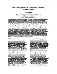
A cut in G = (V, E) i.e., an edge set C of the form C = δ(W ), W ⊆ V , where δ(W ) = {e ∈ E | v ∈ W, w ∈ V \ W }, partitions V into V = V + ∪ V − (V + ∩ V − = ∅), where V + and V − are called the different shores of the cut. Any home-away assignment corresponds to a cut in G such that, by [F2], (i, j) ∈ V + if and only if (tij , j) ∈ V − and |E| − |C| is the number of breaks. This condition is modeled by stipulating that (i, j) and (tij , j) belong to different shores of the cut. We could model this by assigning a capacity of 1 to all edges of G introduced so far and a value of M ≥ n(n − 2) + 1 to all n(n−1) such pairs of nodes: Fig. 2 2 shows the graph G resulting from this transformation for the instance given in Fig. 1(a).

2

3

4

5

6

7

8

1

7

5

4

3

8

6

7

1

8

6

2

5

4

5

8

1

2

7

6

3

4

6

2

1

8

3

7

8

5

7

3

1

4

2

3

2

6

8

4

1

5

6

3 2 5 4 7 thin edges have capacity 1, fat edges have capacity M Fig. 2. Result of the big-M transformation

1

4


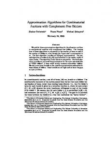
The choice of M would trivially guarantee a correct model. Namely, if the maximum capacity cut with these edge weights has value ∆, then assigning “+” to tij with (i, j) ∈ V + and “−” to tij with (i, j) ∈ V − gives a schedule with the minimum number of ∆ − n(n−1) M 2 breaks. But, due to a result of Barahona and Mahjoub [10] we can do much better. If we switch the signs of the capacities of all edges in the star of any node v in G, the maximum capacity cut induces a maximum capacity cut with the original capacities in which v changes shores and all other nodes stay at their shore. Therefore, for each edge with capacity M we switch the capacity of the star of one of its end-nodes. The resulting edge with capacity −M will be in no maximum cut, so we can nodes and n(n − 2) edges contract the edge. We obtain a maximum cut instance with n(n−1) 2 with capacities either 1 or −1. The result for our example is shown in Fig. 3, in which we have (arbitrarily) chosen to switch the cut of the lower indexed vertex each time.)

2

3

4

5

6

7

8

1

1

1

1

1

1

1

7

7

5

4

3

8

6

3

2

2

2

2

2

2

5

8

8

6

7

5

4

4

4

3

3

4

3

3

8

6

7

8

8

6

7

6

5

6

7

5

4

5

thin edges have capacity 1, fat edges have capacity −1 Fig. 3. Result of the transformation

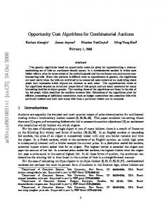
The same graph is displayed in Fig. 4 along with a cut of maximum capacity 22 that is indicated by white and grey nodes, respectively. By backward transformation, this cut corresponds to the home-away assignment displayed in Fig. 1(a) with 8 breaks, which proves our claim that 8 breaks is minimum for this instance. 1.3

Computational Results

For the computation of maximum capacity cuts we have used an implementation of the branch-and-cut algorithm described in [9] that was reimplemented by Martin Diehl using the ABACUS software [42], version 2.3 with Cplex 6.5 as an LP-Solver. The same implementation was used successfully in, e.g., [24, 25] for computing ground states of Ising spin glasses.


2

3

4

5

6

7

8

1

1

1

1

1

1

1

7

7

5

4

3

8

6

3

2

2

2

2

2

2

5

8

8

6

7

5

4

4

4

3

3

4

3

3

8

6

7

8

8

6

7

6

5

6

7

5

4

5

capacity 1, not in the cut capacity 1, in the cut capacity -1, not in the cut capacity -1, in the cut

Fig. 4. A cut of maximum capacity 22

5

6


The instances were created by computing optimal ((n − 2)-breaks schedules) by Schreuder’s procedure and permuting the columns randomly. For each site, we created five random schedules and applied the branch-and-cut algorithm. The results displayed in Table 1 were obtained on a 296MHz Sun Ultra SPARC machine. size time (sec) no. breaks n minimum average maximum minimum maximum 14 0.2 0.26 0.5 24 26 16 0.2 0.77 2.5 26 34 18 1.0 2.30 18.3 38 44 20 1.4 8.10 49.2 46 56 22 2.9 10.20 44.4 56 64 24 6.7 85.73 507.5 66 78 26 15.9 465.36 5185.7 82 92 Table 1. Computational Results

We also solved one real world instance, namely the current Bundesliga (first national German soccer league) instance. There are 18 teams and we found that the schedule is already optimal at 16 breaks! We do not have access to the instances used in the computational studies by Régin and Trick, however, at the time of writing this, it seems that Trick’s approach is slightly ahead in solving 22 teams instances in about 1 hour on a 266 MHz machine. Apparently, our approach is able to handle larger instances easily1 .

2

A Bit of History

Mathematical Programming, originating as a scientific discipline in the late forties, is concerned with the search for optimal decisions under restrictions. The most prominent mathematical models include linear programming, (mixed) integer linear programming and combinatorial optimization with linear objective function. A surprisingly large variety of problems in economics, mathematics, computer science, operations research and the natural sciences can be captured by these models and effectively solved by appropriate software. Years before computer science emerged as a scientific discipline, the protagonists of mathematical programming, who were mainly applied mathematicians or mathematically oriented economists, aimed at the development of algorithms that could solve the problem instances, in the beginning primarily economic and military planning applications, by hand calculations and, when electronic computers became available in the early fifties, via computer software. Linear Programming The father of linear programming is George B. Dantzig, who proposed the model maximize cT x subject to Ax ≤ b x≥0 1

(1)

We would like to thank Michael Trick for teaching us the break minimization problem and sharing his insights with us.


7

where c ∈ IRn , A ∈ IRm×n , b ∈ IRm , and invented the celebrated simplex algorithm for its solution. In the first sentence of his textbook “Linear Programming and Extensions” [20] he states: “The final test of a theory is its capacity to solve the problems which originated it” and before he proceeds to the acknowledgments, he writes: “The viewpoint of this work is constructive. It reflects the beginning of a theory sufficiently powerful to cope with some of the challenging decision problems upon which it was founded.” Not only the model and the simplex algorithm have pertained to this day, but also the philosophy he summarizes in these two sentences remained a leitmotif for mathematical programmers until today, as Michel Balinski puts it in [6]: “First the real problems, then the theory . . . ”, and we can safely add: “. . . and then implementing and testing it on the real problems.” The simplex algorithm was implemented in the US National Bureau of Standards on the Standards Eastern Automatic Computer (SEAC) as early as 1952, and computational testing and comparison with competing methods was performed in a way that meets today’s standards for such experiments. Slightly later, around 1954, William Orchard-Hays of the RAND Corporation designed the first commercial implementations of the (revised) simplex algorithm for the IBM CPC, IBM 701 and IBM 704 machines. Also direct commercial applications in the oil industry were started as early as 1952 by A. Charnes, W.W. Cooper and B. Mellon [13]. Integer Programming It became soon clear, though, that in real problems integrality of some of the decision variables is required. If an optimum plan of activities requires using 1.3 airplanes, this makes no sense. Also, very often yes/no decisions are desired that can be modeled using binary variables. So the (mixed) integer (binary) linear programming model is the linear programming model in which (some) variables are required to take integral (binary) values. In 1958, Ralph Gomory [30] presented an elegant algorithmic solution to the integer linear programming problem that was later refined to the mixed integer case. Interestingly, he not only invented the “cutting plane” method and proved its finiteness and correctness, but he also implemented it in the same year on an E 101 and an IBM 704 computer in the then brandnew FORTRAN language, in order to see how it performs. Unfortunately, the early experiments where not very satisfactory in terms as practical efficiency, and Gomory’s cutting plane method, even though appreciated for its theoretical beauty, was not recommended for practical computations until only a few years ago Balas, Ceria, Cornuéjols, and Natraj [4] gave computational evidence that it should be reconsidered. Instead, the branch-and-bound method proposed by A.H. Land and A.G. Doig in 1960 [45] became the method of choice in all commercial computer codes that were provided by many computer companies starting with linear programming in the sixties and mixed integer programming in the seventies. Combinatorial Optimization In combinatorial optimization with a linear objective function, the task consists of selecting from a family of subsets F ⊆ 2E ofP a finite ground set E one F ∈ F that maximizes (minimizes) a linear objective function e∈F ce for coefficients ce ∈ IR, e ∈ E. Mathematically, this is trivial, because an optimizing set F can be found by finite enumeration, however such a strategy is clearly unsatisfiable for practical computation. Some of the finest algorithms in computer science and mathematical programming that have been formulated for problems like the minimum spanning tree problem, the shortest path problem, or the matching problem by Kruskal [44], Dijkstra [26] and Edmonds [27], respectively, fit into this framework, as well as many others in combinatorics and (hyper-) graph theory.

8


In our examples, the finite ground set E consist of the edges of a graph G and the feasible solutions are the spanning trees, the paths connecting two specified nodes and the matchings in G, respectively. Branch-and-Cut Unlike these examples, most examples with practical applications have turned out to be NP-hard. Nevertheless, an obvious connection to binary integer programming leads to an algorithmic methodology that has been found out to be able to solve real world instances to optimality anyway. Any F ⊆ E is characterized by its characteristic vector χF ∈ {0, 1}E in which χF e = 1 if and only if e ∈ F . Passing from the feasible subsets to their characteristic vectors, it is usually not hard to define the problem as a binary linear programming problem, whereas it is usually a long way, theoretically and in terms of implementation effort, to make the well developed linear programming techniques exploitable in effective computation. We demonstrate this on a prominent example, the traveling salesman problem (TSP), in which the task is to find Hamiltonian cycle (“tour”) with minimum total edge weight in a complete undirected graph. Incidentally, this is the problem for which now commonly used optimization techniques were first outlined by G.B. Dantzig, D.R. Fulkerson and S.M. Johnson in 1954 [21]. If xij is a variable corresponding to the edge connecting nodes i and j, and cij is the weight (length) of this edge, then minimize subject to

P

cij xij

ij∈E P

= 2 for all i ∈ V

xij

j∈V

P

xij ≥ 2 for all S ⊂ V, 3 ≤ |S| ≤

i∈S,j∈V \S

0 ≤ xij ≤ 1 xij ∈ {0, 1}

j

|V | 2

k

(2)

for all ij ∈ E for all ij ∈ E

is an integer programming formulation in which the equations make sure that in the solution every node has degree two and the inequalities, called subtour elimination constraints, guarantee that we do not obtain a collection of subtours. The variables with value 1 in an optimum solution of this integer program are in one-to-one correspondence with the edges of an optimum tour. Discarding the integrality conditions, we obtain a linear programming relaxation (subtour relaxation) that can be used in a branch-and-bound environment: A simple scheme would solve the relaxation at every subproblem in which some variables have been set to 0 or 1. If the solution is not integral, two new subproblems, with one non-integral variable set to 1 in one and to 0 in the other, are created in a branching step. However, this linear programming relaxation contains an exponential number of constraints (Θ(2n )) for an instance on n nodes. This leads to the idea to solve the relaxation with a small subset of all constraints, check if the optimum solution violates any other of the constraints, and if so, append them to the relaxation. Thus we get a cutting plane method at each node of the enumeration tree that arises by branching. This method is called branch-and-cut. It was first formulated for and successfully applied to the linear ordering problem Grötschel, J¨ unger, and Reinelt in [32]. The first state-of-theart branch-and-cut algorithm was published by Padberg and Rinaldi in [54] where it was used to solve large TSP instances. The major new features of the Padberg-Rinaldi algorithm are the branch-and-cut approach in conjunction with the use of column/row generation/deletion techniques, sophisticated separation procedures and an efficient use of the LP optimizer.


9

There are many ways to strengthen the subtour relaxation by further classes of inequalities. Identifying some of them that violate a given fractional solution is called the separation problem. This problem can be solved in polynomial time for the subtour elimination constraints. Of course, it would be desirable to compute a complete description by linear equations and inequalities of the convex hull of the characteristic vectors of tours, which is the TSP polytope n PTSP = conv{χT ∈ {0, 1}En | χT is the characteristic vector of a Hamiltonian cycle in Kn .}

Here, Kn = (Vn , En ) denotes the complete undirected graph on n nodes. Such a description exists by classical theorems of Minkowski and Weyl. However, results of Karp and Papadimitriou [43] make it unlikely that we can compute it except for very small n. Even when we restrict ourselves to non-redundant inequality systems, in which each inequality defines a facet of the polytope, i.e., a proper face of maximum dimension, the number of needed inequalities is enormous, e.g., 42,104,442 for n = 9 and at least 51,043,900,866 for n = 10 [16, 15]. The field of polyhedral combinatorics deals with identifying subsystems of such complete and non-redundant linear descriptions. In order to make a subclass computationally exploitable, we must devise according separation algorithms, or at least useful heuristics, if the problem is proven to be or appears to be hard. Computer implementations for branch-and-cut algorithms for the TSP have been devised by a few research groups, the first, in which the term “branch-and-cut” was used for the first time, by Padberg and Rinaldi [53]. Such programs solve most instances with a few hundred cities routinely and also some instances with a few thousand cities, see [37] for a recent survey of the theory and practice of this method for the TSP, [39] for an account how the same methodology can be applied to other combinatorial optimization problems, and [12] for a recent annotated bibliography on branch-and-cut algorithms. The first essential ingredient that makes such an approach work consists of a theoretical part that requires creative analytical investigations on identifying appropriate classes of inequalities (polyhedral combinatorics) and the design of separation algorithms. Together with the implementation of the separation algorithms this is highly problem specific (see Section 4.1). The second ingredient is integrating the separation software into a cutting plane framework and this into an enumerative frame. This latter part is much less problem specific but requires a considerable implementation effort that can be reduced by an appropriate software system.

Branch-and-Price We use the binary cutting stock, another example of a combinatorial optimization problem, in order to introduce a special version of “branch-and-cut”, namely branch-and-price. In branch-and-price the cut generation phase never takes place, but only columns are dynamically added to the LP relaxation at every node of the enumeration tree. Further details on this approach will be given in Section 4.2. In the binary cutting stock problem, a set of n rolls of lengths a1 , a2 , . . . an has to be cut out of base rolls with length L. The problem is to determine a cutting strategy that minimizes the number of base rolls used. In 1961, P.C. Gilmore and R.E. Gomory [29] proposed thePfollowing model: The vector b ∈ {0, 1}n represents a cutting pattern for a n n×m base roll if represent all i=1 ai bi ≤ L. Let the columns of the matrix B ∈ {0, 1} possible cutting patterns. Then the problem can be modeled as the following binary linear

10


programming problem: minimize

m P

subject to

j=1 m P

zj bij zj = 1 for all i ∈ {1, 2, . . . , n}

(3)

j=1

0 ≤ zj ≤ 1 zj ∈ {0, 1}

for all j ∈ {1, 2, . . . , m} for all j ∈ {1, 2, . . . , m}

In any feasible solution zj = 1 if and only if the j-th cutting pattern is used. In contrast to our previous example in which we had a polynomial numbers of variables and an exponential number of constraints, here we have the opposite situation. If we solve the problem on a small subset of the columns, we have to make sure that the missing columns can be safely assumed to be associated with 0 components of the optimum vector z. The simplex algorithm does not only give us a basic feasible solution (geometrically this corresponds to a vertex of the polyhedron defined by the restrictions) but P also a short certificate for optimality n consisting of a quantity yi for each row i such that i=1 bij yi ≤ 1 for all cutting patterns T B·j = (b1j , b2j , . . . , bnj ) that are present in the chosen subset. In order to determine if the same relation holds for all missing cutting patterns as well we can solve the knapsack problem n P maximize yi bi subject to

i=1 n P

ai bi ≤ L

(4)

i=1

bi ∈ {0, 1} for which effective pseudo-polynomial algorithms exist. If the maximum is at most 1, our solution is optimal for the complete problem, otherwise the optimum pattern b1 , b2 , . . . , bn found by the algorithm is appended as a new column to the formulation. This process of evaluating the missing columns is called “pricing” in linear programming terminology, and embedding the method into an enumerative frame leads, as we already said, to a branchand-price algorithm. Cutting and pricing can be combined (and they are in all published state-of-the-art algorithms for the optimum solution of the TSP) even when the problem involves, like in this example, exponentially many variables. This methodology is called branch-and-cut-and-price and will be described in more details in Section 4.2.

3

Components of Branch-and-Cut

Fig. 5 shows a flowchart of a generic branch-and-bound algorithm for a minimization problem. A basic branch-and-cut algorithm is a branch-and-bound algorithm in which the bounds are solutions of LP-relaxations that are iteratively strengthened by problem specific cutting planes at every node of the enumeration tree. This feature incurs several technicalities that make the design and implementation of branch-and-cut algorithms a nontrivial task. In this section we will present a basic branch-and-cut algorithm, address such technical details and give some ideas for an efficient implementation that proved to be useful in practice. A first outline of a basic branch-and-cut algorithm is given in the flowchart of Fig. 6 in which the dashed clusters correspond to boxes in the flowchart of Fig. 5. Roughly speaking, the two leftmost of the four columns describe the cutting plane phases within a single subproblem, the third column shows the preparation and execution of a branching operation, and in the rightmost column, the fathoming of a subproblem is performed. We give informal


START

STOP

INITIALIZE

OUTPUT

y

COMPUTE GLOBAL UPPER BOUND gub AND LOCAL LOWER BOUND llb

n

11

n list empty

gub > llb

SELECT

y

feasible

n

BRANCH

FATHOM

y

Fig. 5. Flowchart of a branch-and-bound algorithm for minimization problems. Figure 1.

Flowchart of the branch and bound algorithm.

explanations all steps of the together some problem specific details. In of theFigure 1, Before we startofexplaining theflowchart

owchart of thewith branch and bound algorithm remainder of this section the underlying optimization problem is always assumed to be a we introduce some terminology concerning upper bounds (derived fromof solving relaxations) minimization problem. Moreover, during the description of the basic version the algorithm assume that in all its phases the setfeasible of variables remains unchanged. each local, and lowerwebounds (obtained by nding solutions). We call Inanparticular, upper bound LP problem has a fixed number of columns, while the number of rows increases or decreases if it is only valid for a subproblem, and global, if it is a bound for the original problem. after the modules called SEPARATE and ELIMINATE have been executed (see Section 3.3). By solving ofalgorithm, the current weareobtain a the local upper bound lub The a fullrelaxation version of the whereproblem, also columns added to LP, is described in Section 3.5. function value of the original problem. If the solution found for the for the objective of the components of theoriginal presentedproblem algorithmic are problem relaxation Although happensmost to be feasible for the (inframework which case it is also the independent in general, we choose the TSP as our main example. This has several optimumsons. solution of the subproblem) and has higher objective function valuerea-than any First, the TSP is probably one of the most prominent combinatorial optimization feasible solution foundit issothefar,prototype it is memorized problems, then problem for and whichthe in global [53] and lower [54] the bound superiorityglb of for the branch-and-cut over the other known approaches was shown, and finally implementations objective function value is increased accordingly. of state of the art TSP solver like the one of J¨ unger/Naddef/Reinelt/Thienel [50] or AppleA branch and bound algorithm maintains a listtechniques of subproblems the original probgate/Bixby/Chv´ atal/Cook [2] contain all algorithmic we want toofdemonstrate. Adaptions of these techniques easily be applied toitself. branch-and-cut for other step the lem, which is initialized with thecan original problem In each algorithms major iteration combinatorial optimization problems. algorithm selects a subproblem from this list, computes a local upper bound for this subIn our description, we proceed as follows. First we describe the local enumerative of thedoes not problem,algorithm, and tries to improve the global lower bound. If the upperpart bound i.e., we discuss in detail how branching and selection operations can be performed. exceed the global lowerthebound, thein acurrent subproblem is fathomed, its solution Then we explain work done subproblem of the enumeration. We also because discuss sparse techniques lead known to column generation. cannot begraph better than which the best feasible solution. Otherwise we check if the optimal solution of the relaxation of the subproblem is a feasible solution of the original problem. In this case we have solved the subproblem and thus, it is fathomed. If the local upper bound exceeds the global lower bound and no feasible solution was found for the current problem, we perform a branching step by splitting the current

12


START NEW NODE

INITIALIZE

INITIALIZE NEW NODE

SOLVE LP

infeasible LP

y

SETBYLOGIMP

n n

y gub > llb

gub > lpval y

n

n y contradictions

EXPLOIT LP

n y

y feasible

list empty

n y

SELECT

tailing off n

BRANCH

FATHOM

n y

FIX

new values n contradictions

FIX AND SET

contradictions

y

FIX AND SET

y

n SEPARATE

new constraints

y

ELIMINATE

n

n gub > lpval

y

feasible

y

n

OUTPUT

STOP

Figure 2.

Flowchart of the branch and cut algorithm.

Fig. 6. Flowchart of a basic branch-and-cut algorithm.

13


13

There are two major ingredients of a branch-and-bound algorithm, the computation of global upper and local lower bounds. The lower bounds are produced by performing an ordinary cutting plane algorithm for each subproblem. Two basic techniques for the computation of upper bounds (corresponding to feasible solutions of the original problem) are currently being used. The first method is to compute a good upper bound by some heuristics before the root node of the complete branch-and-cut tree is processed. Later this bound can only be improved, if the solution of a linear program is the characteristic vector of a better feasible solution. The other method is the computation of upper bounds in the cutting plane phase by exploiting fractional LP-solutions. This technique may require more running time spent for heuristics, yet may decrease the total running time, since the size of the enumeration tree may be smaller. For the TSP, we describe how the LP-solution can be utilized in oder to find good feasible solutions, i.e., upper bounds. 3.1

Terminology

Before going into details, we have to define some terminology. That is used not only in this section but also in Section 5 where we discuss the object oriented software framework ABACUS which implements the generic branch-and-cut algorithm of Fig. 6. Due to a corresponding naming scheme in ABACUS every algorithmic component or variable of the described algorithm is easily identified as a module, variable or data structure in the software. Since in a branching step like in a branch-and-boundalgorithm two (or more) new subproblems are generated, the set of all subproblems can be represented by a binary (k-nary) tree, which we call the branch-and-cut tree. Hence we call a subproblem a branch-and-cut node. Fig. 7 shows an example of a branch-and-cut tree. We distinguish between four types of branch-and-cut nodes. The node which is currently being processed is called the current branch-and-cut node. The other unfathomed leaves of the branch-and-cut tree still have to be processed and are called the active nodes. Finally, there are the already processed non-active nodes. A non-active node can either be fathomed or not fathomed. Each variable has one of the following attributes during the computation: atlowerbound, basic, atupperbound, settolowerbound, settoupperbound, fixedtolowerbound, fixedtoupperbound. When we say that a variable is fixed to zero (lower bound) or one (upper bound), it means that it is at this value for the rest of the computation. If it is set to zero (lower bound) or one (upper bound), this value remains valid only for the current branch-and-cut node and all branch-and-cut nodes in the subtree rooted at the current one in the branch-and-cut tree. The conditions for fixing and setting variables will be explained later in Section 3.2. The meanings of the other attributes are obvious: As soon as an LP has been solved, each variable which has not been fixed or set receives one of the attributes atlowerbound, basic or atupperbound by the revised simplex method with lower and upper bounds. Finally, the variable lpval always denotes the optimal value of the last LP that has been solved, which is also a local lower bound llb for the currently processed node, the global variable gub (global upper bound) gives the value of the currently best known feasible solution. The minimum lower bound of all active branch-and-cut nodes and the current branch-and-cut node is the global lower bound glb for the whole problem. The subtree rooted at the highest common ancestor of all active and the current branch-and-cut nodes is called the remaining branch-and-cut tree. Therefore, we call this highest common ancestor also the root of the remaining branch-and-cut tree and the local lower bound of this node is called rootlb. The difference between glb and rootlb will be discussed below.

14


Fig. 7. Branch-and-cut tree with different nodes.

Like in branch-and-bound terminology we call a subproblem fathomed, if the local lower bound lpval of this subproblem is greater than or equal to the global upper bound gub, or if the subproblem becomes infeasible (e.g., if branching variables have been set in a way that the subproblem does not contain any feasible solution), or if the subproblem is solved, i.e., the solution of the LP-relaxation is a feasible solution of the original problem. In many applications all objective function coefficients are integer. In that case all feasible solutions have an integer value. Therefore, all terms of the computation that express a lower bound may be rounded up, e.g., one can fathom a node with global upper bound gub and local lower bound llb, if dllbe ≥ gub. For some specially structured problems it might be valid to round up the local lower bound more than one unit, for example to the next even (or odd) integer. These extended roundings should always be applied since tightening the bounds may be essential for practical efficiency. The branch-and-cut algorithm consists of three different parts: The enumerative frame, the computation of lower bounds and the computation of upper bounds. It is easy to identify the boxes of the flowchart of Fig. 5 with the dashed boxes of the flowchart of Fig. 6. The central part is the lower bounding part that is performed after the selection of a new current subproblem. It consists of trying to solve the current problem by optimizing over LP-relaxations that are tightened by adding cutting planes. This bounding part is left, – – – – –

if the local lower bound is greater than or equal to the global upper bound, if the LP-solution is the characteristic vector of a feasible solution, if no more cutting planes can be generated, if infeasibility of the current subproblem is detected, if the upper bound does not decrease significantly, although cutting planes are added (tailing off).

It is advantageous, although not necessary for the correctness of the algorithm, to reenter the bounding part if variables are fixed or set to new values by FIX AND SET, instead of creating new subproblems in BRANCH.


15

Fig. 8. Root change of the remaining branch-and-cut tree.

3.2

Enumerative Frame

The enumerative frame consists of all parts of the branch-and-cut algorithm except the bounding part (the leftmost dashed box of Fig. 6). INITIALIZE. During the computation the algorithm stores a set of active branch-and-cut nodes. After input of the problem, the set of active branch-and-cut nodes is initialized as the empty set. To initialize the global upper bound gub, feasible solutions are computed by some heuristic methods. For the TSP, we can construct a tour with the nearest neighbor heuristic and improve it with a Lin-Kerninghan Procedure [46]. Afterwards the root node of the complete branch-and-cut tree becomes the current branch-and-cut node which is now processed by the bounding part. BOUNDING. The computation of the lower and upper bounds is outlined in the sections 3.3 and 3.4. We continue the explanation of the enumerative frame at the ordinary exit of the bounding part (at the end of the first column of the dashed bounding box). If the current branch-and-cut node cannot contain a feasible solution that is better than the best known one (lpval ≥ gub), or the final LP-solution is the characteristic vector of a feasible solution (feasible), the node is fathomed. Otherwise a branching operation and the selection of another branch-and-cut node for further processing (third column of the flowchart) is prepared. FIX AND SET. The routine FIX AND SET of Fig. 6 consists of the four procedures FIXBYREDCOST, FIXBYLOGIMP, SETBYREDCOST and SETBYLOGIMP. If a branching operation is prepared, and the current branch-and-cut node is the root node of the branch-and-cut tree, the reduced cost of the non-basic variables obtained from the LP-solver can be used to fix them forever at their current values by the routine FIXBYREDCOST. Namely, if for an edge e the variable xe is non-basic and the reduced cost is re , we can fix xe to zero if xe = 0 and rootlb + re > gub and we can fix xe to one if xe = 1 and rootlb − re > gub. During the computational process, the value of gub decreases, so that at some later point in the computation, one of these criteria can be satisfied, even though it is not satisfied at the current point of the computation. Therefore, each time when we get a new root of the remaining branch-and-cut tree, we make a list of candidates for fixing of all non-basic variables along with their values (0 or 1) and their reduced costs and update rootlb. We get a new root of the remaining branch-and-cut tree, if all nodes in all subtrees except one subtree of the old root are fathomed (see Fig. 8).

16


Since storing these lists in every node, which might eventually become the root node of the remaining active nodes in the branch-and-cut tree, would use too much memory space, we process the complete bounding part a second time for the node, when it becomes the new root. If we could initialize the constraint system for the recomputation by those constraints that were present in the last LP of the first processing of this node, we would need only a single call of the simplex algorithm. However, this would require too much memory. So we initialize the constraint system with the constraints of the last solved LP. As some facets are separated heuristically, it is not guaranteed that we can achieve the same local lower bound as in the previous bounding phase. Therefore we not only have to use the reduced costs and statuses of the variables of this recomputation, but also the corresponding local lower bound as rootlb in the subsequent calls of the routine FIXBYREDCOST. If we initialize the basis by the variables contained in the best known solution and call the primal simplex algorithm, we can avoid phase 1 of the simplex method. Of course this recomputation is not necessary for the root of the complete branch-and-cut tree, i.e., the first processed node. The list of candidates for fixing is checked by the routine FIXBYREDCOST whenever it has been freshly compiled or the value of the global upper bound gub has improved since the last call of FIXBYREDCOST. FIXBYREDCOST may find that a variable can be fixed to a value opposite to the one it has been set to (contradiction). This means that earlier in the computation, somewhere on the path of the current branch-and-cut node to the root of the branch-and-cut tree, we have made an unfavorable decision which led to this setting either directly in a branching operation or indirectly via SETBYREDCOST or SETBYLOGIMP (to be discussed below). Before starting a branching operation and if no contradiction has occurred, some fractional (basic) variables may have been fixed to new values (0 or 1). In this case we solve the new LP rather than performing the branching operation. FIXBYLOGIMP. After variables have been fixed by FIXBYREDCOST, we call FIXBYLOGIMP. In contrast to reduced cost fixing this is not problem independent. For the TSP, this routine might try to fix more variables by logical implication as follows: If two edges incident to a node v have been fixed to 1, all other edges incident to v can be fixed to 0. Like in FIXBYREDCOST, contradictions to previous variable settings may occur. If variables are fixed to new values, we proceed as explained in FIXBYREDCOST. In principle also fixing or setting variables to zero could have logical implications. If all incident edges of a node but two are fixed or set to zero, these two edges can be fixed or set to one. However, this occurs quite rarely and can therefore be disregarded. SETBYREDCOST. While fixings of variables are globally valid for the whole computation, variable settings are only valid for the current branch-and-cut node and all branch-andcut nodes in the subtree rooted at the current branch-and-cut node. SETBYREDCOST sets variables by the same criteria as FIXBYREDCOST, but based on the local reduced cost and the local lower bound llb of the current subproblem rather than “globally valid reduced cost” and the lower bound of the root node rootlb. Contradictions are possible if in the meantime the variable has been fixed to the opposite value. In this case the current branch-and-cut node is fathomed. SETBYLOGIMP. This routine is called whenever SETBYREDCOST has successfully set variables, as well as after a SELECT operation. It tries to set more variables by logical implication as follows: If two edges incident to a node v have been set or fixed to 1, all


17

other edges incident to v can be set to 0 (if not fixed already). Like in SETBYREDCOST, all settings are associated with the current branch-and-cut node. If variables are set to new values, we proceed as explained in FIXBYREDCOST. After the selection of a new node in SELECT, we check if the branching variable of the father is set to 1 for the selected node. If this is the case, SETBYLOGIMP may also set additional variables. BRANCH. Branching in general is splitting the current subproblem in two or more new one. There are many different strategies to achieve this. For example: – – – –

a fractional 0/1 variable is set to 0 and 1 upper and lower bounds for integer variables are changed dividing the polytope by hyperplanes other problem specific strategies

If we choose the first method some variable is chosen as the branching variable and two new branch-and-cut nodes, which are the two sons of the current branch-and-cut node, are created and added to the set of active branch-and-cut nodes. In the first son the branching variable is set to 1, in the second one to 0. If no constraints of the integer programming formulation are violated, then there is at least one fractional variable that is a reasonable candidate for a branching variable. However if a constraint of the integer programming formulation is violated, it is possible that all variables have an integral LP-value, yet the LP-solution is not a feasible solution of the original problem. In this case a variable with an integral LP-value has to be chosen as branching variable. There is a variety of different strategies for the selection of the branching variable, so that we can present here only some of them. Let x be the solution of the last solved LP. 1. Select a variable with value close to 0.5 that has a big objective function coefficient in the following sense. Find L and H with L = max{xe | xe ≤ 0.5, e ∈ E} and H = min{xe | xe ≥ 0.5, e ∈ E}. Let C = {e ∈ E | 0.75L ≤ xe ≤ H + 0.25(1 − H)} be the set of variables with value “close” to 0.5. From the set C the variable with maximum cost is selected, i.e., with maximum objective function coefficient. 2. Select the variable that has an LP-value closest to 0.5. 3. Select the fractional variable (if available) that has maximum objective function coefficient. 4. If there are fractional variables that are equal to 1 in the currently best known feasible solution, select the one with maximum cost of them, otherwise, apply strategy 1. 5. Select a fractional variable (if available) that is closest to one, i.e., find a variable e? with xe? = max{xe | xe ≤ 0.999}. 6. Select a set L of promising branching variable candidates. Let Ax ≤ b be the constraint system of the last solved LP. Solve for each variable i ∈ L the two Linear Programs v0i = max{cT x | Ax ≤ b, xi = 0} v1i = max{cT x | Ax ≤ b, xi = 1} and select the branching variable b with max{v0b , v1b } = min max{v0i , v1i }. i∈L

Some running time can be saved if instead of the solution of the Linear Programs to optimality only a restricted number of iterations of the simplex-method is performed. Then the objective function value might already indicate the “quality” of the branching variable, especially if a steepest edge pivot selection criterion is applied.

18


Computational experiments for the strategies (1) and (3) – (5) applied to the TSP can be found in [41]. Other branching variable selection strategies can be found in [5]. Instead of partitioning the set of feasible solutions by branching on a variable, it is also possible to use a hyperplane intersecting the polytope defined by the current subproblem. This alternative way of branching was proposed for the first time in [18] and used with a problem specific hyperplane for the TSP. Another modification of the branching process is branching on k ≥ 2 variables or hyperplanes. In this case we get a 2k -nary instead of a binary branch-and-cut tree.

SELECT. A branch-and-cut node is selected and removed from the set of active branchand-cut nodes. If the list of active branch-and-cut nodes is empty, the best known feasible solution is the optimum solution. Otherwise the selected node is processed. After a selection the set variables (including the branching variables) must be adjusted. If it turns out that some variable must be set to 0 or 1, yet has been fixed to the opposite value in the meantime, we have a contradiction. In this case the branch-and-cut node is fathomed. If the local lower bound llb of the selected node exceeds the global upper bound gub, the node is fathomed immediately and the selection process is continued. Up to now we have not specified which node is selected from the set of active branch-andcut nodes. There are three well-known enumeration strategies in branch-and-bound(branchand-cut ) algorithms: depth-first search, breadth-first search and best-first search. We define the level of a branch-and-cut node B as the number of edges on the path from the root of the branch-and-cut tree to B. In the case of depth-first search a branch-and-cut node with maximum level in the branch-and-cut tree is selected from the set of active nodes in SELECT, whereas in breadth-first search a subproblem with minimum level is selected. In best-first search the “most promising” node becomes the current branch-and-cut node. For a minimization problem the node with maximum local lower bound among all active nodes is often considered as most promising. Computational experiments for the TSP (see [41]) show that depth-first search is an enumeration strategy with the “risk” of spending a lot of time in a branch of the tree, which is useless for computing better upper and lower bounds. Often the local lower bound of the current subproblem exceeds the objective function value of an optimum solution, however, this node cannot be fathomed, because no good upper bound is known. The same phenomenon occurs also sometimes when using breadth-first search, but it is very rare if the enumeration is performed in best-first search order.

FATHOM. If for a node the global upper bound gub does not exceed the local lower bound llb, or a contradiction occurred, or an infeasible branch-and-cut node has been generated, or if the LP-solution is an characteristic vector of a feasible solution, the current branchand-cut node is deleted from further consideration. Even though a node is fathomed, the global upper bound gub may have changed during the last iteration, so that additional variables may be fixed by FIXBYREDCOST and FIXBYLOGIMP. The fathoming of nodes in FATHOM may lead to a new root of the branch-and-cut tree for the remaining active nodes.

OUTPUT. The currently best known solution, which is either an optimum solution or satisfies a desired guarantee requirement, is written to an output file.


3.3

19

Computation of Local Lower Bounds

The computation of local lower bounds consists of all elements of the leftmost dashed bounding box of Fig. 6 except EXPLOIT LP. In EXPLOIT LP the upper bounds are updated, if the solution of the Linear Program is the characteristic vector of a better feasible solution. Also improvement heuristics, using information from the LP-solutions, can be incorporated here as suggested in Section 3.4. For the computation of lower bounds LP-relaxations are solved iteratively, violated valid inequalities are added, and non-binding constraints are deleted from the constraint matrix. In this section we will also point out that an additional data structure for inequalities, called pool, is very useful, although not necessary for the correctness of the algorithm. For now, we can think of a pool just as a collection of constraints or variables. The active inequalities are the ones in the current LP and are both stored in the pool and in the constraint matrix, whereas the inactive constraints are only present in the pool. The pool is initially empty. If an inequality is generated by a separation algorithm, it is stored both in the pool and added to the constraint matrix. Further details of the pool are outlined in Section 5.3. INITIALIZE NEW NODE. If the current branch-and-cut node is the root node of the branch-and-cut tree the LP is initialized by some small constraint system. Often the upper and lower bounds on the variables are a sufficient choice (e.g., for the MAX-CUT Problem). For the TSP, the degree constraints for all nodes are normally added. Augmenting the initial system by other promising cutting planes can sometimes reduce the overall running time (see [33]). A primal feasible basis derived from a feasible solution can be used as a starting basis in order to avoid phase 1 of the simplex algorithm. Any set of valid (preferably facet defining) inequalities can be used to initialize the first constraint system of subsequent subproblems. Yet, in order to guarantee monotonicity of the values of the local lower bounds in each branch of the enumeration tree, and to save running time, it is appropriate to initialize the constraint matrix by the constraints that were binding when the last LP of the father in the branch-and-cut tree was solved. Since the basis of the father is dual feasible for the initial LP of its sons, phase 1 of the simplex method can be avoided by starting with this basis. The columns of non-basic set and fixed variables can be removed from the constraint matrix to keep the LP small. If their value is non zero, the right hand side of the constraint has to be adjusted, and the corresponding coefficients of the objective function must be added to the optimal value returned by the simplex algorithm in order to get the correct value of the variable lpval. Set or fixed basic variables should not be deleted, because this would lead to a neither primal nor dual feasible basis and require phase 1 of the simplex method. The adjustment of these variables can be performed by adapting their upper and lower bounds. SOLVE LP. The LP is solved by the primal simplex method, if the basis is primal feasible (e.g., if variables have been added) or by the dual simplex method if the basis is dual feasible (e.g., if constraints have been added). The two-phase simplex method is required if the basis is neither primal nor dual feasible. This can happen if constraints necessary for the initialization of the first LP of a subproblem are not available since they had to be removed from the pool as we will describe in Section 5.3. The LP-solver is one of the bottlenecks of a branch-and-cut algorithm. Sometimes more than 90% of the computation time is spent in this procedure. Today, efficient implementations of the simplex method, like Cplex [17] or XPress [67] are competitive on solving Linear

20


Programs from scratch. However, a branch-and-cut algorithm requires a LP-solver with very efficient post-optimization routines. The simplex method satisfies all the requirements of a branch-and-cut algorithm and it is used by nearly all implementations of cutting plane algorithms. Therefore we have outlined the algorithm in this section under the assumption that the simplex method is used. Since the LPs that have to be solved in a cutting plane algorithm, are often highly degenerate, good pivot variable selection strategies, like the steepest-edge pivot variable selection criterion, are necessary. These degeneracies might even require some preprocessing of the LPs (see, e.g., [33]). EXPLOIT LP. First, we have to check if the current LP-solution is the characteristic vector of a feasible solution. If this is the case we leave the bounding part and fathom the current branch-and-cut node. Otherwise, most implementations of branch-and-cut algorithms proceed with the cutting plane generation phase. However sometimes we can do better by exploiting the fractional LP-solutions to improve the upper bound before additional cutting planes are generated. We will discuss these ideas in Section 3.4. Before the separation phase is performed in SEPARATE, variables may be fixed or set as explained in FIX AND SET. Often it is reasonable to abort the cutting plane part if no significant increase of lpval in the most recent LP-solutions has taken place. This phenomenon is called tailing-off (cf. [54]). If during the last k (e.g., k = 10) iterations in the bounding part, lpval did not increase by more than p % (e.g., p = 0.01), new subproblems are created instead of generating further cutting planes. Good choices for the parameters p and k are both rather problem specific and dependent on the quality of the available cutting plane generation procedures. SEPARATE. The separation phase is the central part of a branch-and-cut algorithm. We try to find violated globally valid (preferably facet-defining) constraints, which are added to the LP. We say an inequality is globally valid, if it is a valid inequality for every subproblem of the branch-and-cut algorithm. We call a constraint locally valid, if it is only a valid inequality of a subproblem S and all subproblems of the subtree rooted at S. It may not always be advantageous to call any available separation algorithm in each iteration of the cutting plane generation. Experiments show that a hierarchy of separation routines is often preferable. Certain separation methods should only be performed, if others have failed. Before calling a time consuming exact separation algorithm, one should attempt to generate cutting planes with faster heuristic methods. However, this hierarchy is rather problem specific so that we cannot give a general recipe for its application. We refer to the publications on specific implementations. The constraint pool provides us with another cutting plane generation technique. Inactive constraints that are violated by the current LP-solution can be regenerated from the pool. Of course this methods requires an efficient algorithm to perform this test and to transform the storage format of the constraint used in the pool into the storage format for the LP-solver. The pool-separation can be advantageous for classes of inequalities for which only heuristic separation routines are available. In this case it can happen that a constraint of this class is violated, yet cannot be identified by the heuristic. However, this cutting plane might have been generated earlier in the computational process (at a different LP solution which has been more “convenient” to our heuristic). If this constraint is still contained in the pool, it can be reactivated now. It can also happen that the pool-separation for a class of constraints is more efficient than a direct separation by a time consuming heuristic or an exact algorithm. Therefore, the pool-separation should always be performed before calling these algorithms. However,


21

for other classes of constraints it can sometimes be observed that the pool-separation is very slow in comparison to direct separation methods. Since the pool can become very large during the computational process, it is necessary to limit the search in the pool for violated inequalities. For instance, the pool-separation can be restricted to some classes of constraints. Therefore the pool-separation should be carefully included into the hierarchy of separation algorithms and it requires many computational tests to find a strategy that is efficient for a specific combinatorial optimization problem. For some combinatorial problems like the MAX-CUT problem, often several hundred violated inequalities can be generated. However, it would be sufficient to add those constraints to the LP that will be binding after the solution of the next LP. Unfortunately we do not know this subset of the generated inequalities. On the other hand, adding all the constraints to the matrix of the LP-solver can slow down the overall computation time. Therefore, depending on the performance of the LP-solver, only a limited number of constraints should be added to the LP. A straightforward approach is just stopping the cut generation when this limit is reached. A more sophisticated method might be generating as many constraints as possible, and afterwards selecting the “best” of them. A simple classification criterion is the degree of violation given by the value of the corresponding slack. For the TSP, Padberg and Rinaldi [54] propose as a measure the distance of the LP-solution from the projection of the cut into the affine space defined by the degree equations. The larger this distance the better the cut, yet, this method is computationally expensive. Other quality measures for cutting planes like the angle of the cut defining hyperplane to the objective function vector have been investigated in [15]. The representation of the inequality for the LP-solver can have significant influence on its running time. For instance, equations of the integer programming formulation can be added to any valid inequality without changing the half-space which it defines. However, the number of the non-zero coefficients in the inequality may differ. Normally, LP-solvers are more efficient if the number of non-zeros in the constraint matrix is small. The solution of the separation problem is very problem specific. Therefore we only want to present an example for the TSP. A polynomial time algorithm for the solution of the exact separation problem of subtour elimination constraints can be directly derived from their definition in Section 2: If the value of the minimum weight cut in the support graph (the graph with the LP-solution as edge weights) is greater than or equal to 2, it is proved that the current LP-solution does not violate any subtour elimination constraint. Each cut with a value less than 2 induces a violated subtour elimination constraint. So the separation problem for subtour elimination constraints reduces to a minimum capacity cut problem for which the practically most efficient solution was given in Padberg and Rinaldi [55] and refined in J¨ unger, Rinaldi, and Thienel [40]. ELIMINATE. If inequalities are added to the constraint matrix of the LP-solver, and no inequalities are eliminated, soon the size of the matrix might become too large to solve the linear programs in reasonable time and even the storage of the constraints in the matrix would require too much memory. Moreover, there are inequalities that become redundant for the rest of the computation. Therefore a strategy is required to maintain a reasonable sized matrix, yet not to eliminate important inequalities. It is an obvious and simple strategy for the elimination of constraints to delete all active inequalities that are non-binding in the last LP-solution from the constraint structure before the LP is solved after a successful cutting plane generation phase. To avoid cycling, i.e., a constraint is eliminated, but already violated after the next LP-solution, either constraints

22


should be only removed if the value of the slack s is big enough (e.g., s > 0.001), or if they are non-binding during several successive LP-solutions. 3.4

Computation of Global Upper Bounds

For most combinatorial optimization problems a host of heuristics is available to compute feasible solutions that provide global upper bounds for the branch-and-cut algorithm. Traditionally the computation of a global upper bound is performed in the procedure INITIALIZE before the cutting plane generation and enumeration phase starts. Later better lower bounds are only found if the LP-solution is the characteristic vector of a feasible solution. However, it can be observed that this happens rather seldomly. Therefore sophisticated heuristics must be applied in INITIALIZE to generate a good lower bound. Otherwise, the enumeration tree may grow too large. In [41] a dynamic strategy, integrated in the cutting plane generation part, for the computation of lower bounds is presented, which we briefly outline. It turns out that the fractional LP-solutions occurring in the lower bound computations in a branch-and-cut algorithm give hints on the structure of optimum or near optimum feasible solutions. The basic requirement for the upper bound computations is efficiency in order not to inhibit the optimization process. While in the first stages high emphasis is laid on providing good feasible solutions, this emphasis is less in the later stages of the computational process. On the other hand, computing upper bounds can always be reasonable since new knowledge about the structure of optimum feasible solutions is acquired (e.g., because of fixed and set variables). Exploiting the LP-Solution. Integer optimal solutions, i.e., characteristic vectors of feasible solutions, will almost never result from the LPs occurring in the branch-and-cut algorithm. But, it can be observed that these solutions, although having many fractional components, give information on good feasible solutions. They have a certain number of variables equal to 1 or 0 and also a certain number of variables whose values are close to 1 or 0. This effect can be exploited to form a starting feasible solution for subsequent improvement heuristics. We show how the information of the LP-values of the variables can be used for the construction of a feasible solution for the TSP. We use the terms edge and variable of the integer programming formulation interchangeably, since they are in a one-to-one correspondence in our examples. First, we check if the current LP-solution is the characteristic vector of a tour. If this is the case we terminate the procedure EXPLOITLP. Otherwise, edges are sorted according to their values in the current LP-solution. We give decreasing priorities to edges as follows: – edges that are fixed or set to 1, – edges equal to 1 or close to 1 in the current LP, – edges occurring in several successive LPs. This list is scanned and edges become part of the tour if they do not produce a subtour with the edges selected so far. This gives a system of paths and isolated nodes which now have to be connected. To this end a savings heuristic of Clarke and Wright [14], originally developed for vehicle routing problems, can be used, since the TSP can be considered as a special vehicle routing problem involving only one vehicle. The previous step gives us a feasible solution that can be improved by local improvement heuristics like Lin-Kernighan [46].


23

This heuristic basically consists of successively merging partial tours to obtain a Hamiltonian tour. We select one node as base node and form partial tours by connecting this base node to the end nodes of each of the paths obtained in the selection step and also adding a pair of edges to nodes not contained in any path. Then, as long as more than one subtour is left, we compute for every pair of subtours the savings that is achieved if the subtours are merged by deleting in each subtour an edge to the base node and connecting the two open ends. The two subtours giving the largest savings are merged. Edges that are fixed or set to 0 should be avoided for connecting paths. 3.5

Sparse Solution and Column Generation

Often combinatorial optimization problems involve a very large number of variables, yet a feasible solution is comparatively sparse. For instance, the TSP on a complete graph of n nodes has n2 variables. Yet, a tour consists only of n edges. Hence, the computational process can be accelerated, if a suitable subset of the edges is initially selected and appropriately augmented during the solution of the problem, if this is required for the correctness of the algorithm. However, sparse graph techniques can not be applied to problems with a dense solution structure like the MAX-CUT problem (see Section 4.1). Sparse graph techniques for the TSP have been introduced by Grötschel and Holland [34]. We present techniques exploiting the sparsity of solutions only for combinatorial optimization problems defined on graphs. However this technique can be generalized for other problems, if the structure of the solutions is sparse, suitable subsets of the variables can be computed efficiently, and a method to generate the columns of non-active variables is available. In order to integrate this technique with the basic algorithm described so far, we have to deal with LP problems where not only rows but also columns of the constraint matrix are dynamically created. The resulting more general algorithm that in [54] was called branchand-cut is described in the flowchart shown in Fig. 9. With respect to the basic algorithm, the gray boxes in the flowchart have to be added or changed. A subproblem, in which an infeasible LP is detected, cannot be fathomed at once, but rather it must be checked if the addition of non-active variables can regenerate the feasibility. We explain this process in ADDVARIABLES. Before leaving the bounding part, it has to be verified in PRICE OUT, if the LP-solution computed on the sparse graph is also optimal on the complete graph. Only in this case the variable lpval becomes a local lower bound lub. The application of the routine FIX AND SET has to be performed now more carefully. The procedure SETBYREDCOST can only be applied after an additional pricing step, in which no variable has to be added. This is also the case for FIXBYREDCOST if the root node of the remaining branch-and-cut tree is currently processed. Suitable Sparse Graphs. The initial sparse graph is generated in the procedure INITIALIZE. For the TSP, a good choice for a sparse graph is the k-nearest neighbor graph. Another suitable subset of the edges may be the Delaunay graph (see also [58] and [18]). Figures 10, 11 and 12 show an optimum tour through 127 beer gardens of Augsburg (Germany) together with the 5-nearest neighbor graph and the Delaunay triangulation. If it cannot be guaranteed that the sparse graph contains a feasible solution, it should be augmented by the edges of a solution computed by a heuristic. Padberg and Rinaldi [54] suggest tout court to create a series of feasible solutions heuristically and initialize the sparse graph with all involved edges. In addition to the sparse graph, the edges of the “reserve graph” can be computed. These edges are additional “promising” edges that do not belong to the sparse graph. For instance,

24


START NEW NODE

INITIALIZE

INITIALIZE NEW NODE

y

SOLVE LP

infeasible LP

y

variables added

n

SETBYLOGIMP

ADD VARIABLES

n n

y gub > llb

gub > lpval y

n

n y contradictions

EXPLOIT LP

n y

y feasible

list empty

n y

SELECT

tailing off n

n

BRANCH

pricing time y

FATHOM

n y

PRICE OUT

FIX

new values n

new variables

y

contradictions

y

n FIX AND SET

contradictions

FIX AND SET

y

n SEPARATE

new constraints

y

ELIMINATE

n PRICE OUT

new variables

y

n

n gub > llb

y

feasible

y

n

OUTPUT

STOP

Fig. 9. Flowchart of a branch-and-cut algorithm. Figure 5.

Flowchart of the branch and cut algorithm with sparse graph techniques. 29


25

Fig. 10. Shortest tour through 127 beer gardens in Augsburg (Germany).

Fig. 11. The 5-nearest neighbor graph for the beer gardens in Augsburg contains all but 3 edges of the best tour.

26


Fig. 12. In the Delaunay graph for the beer gardens in Augsburg only 2 edges of the best tour are missing.


27

if the sparse graph is the 5-nearest neighbor graph, a suitable reserve graph is given by the edges that have to be added to get the 10-nearest neighbor graph. The reserve graph can be used in PRICE OUT and ADDVARIABLES. The algorithm starts working on G, adding and deleting edges (variables) dynamically during the optimization process. We refer to the edges in G as active edges and to the other edges as non-active edges. ADD VARIABLES. Variables have to be added to the sparse graph if indicated by the reduced costs (handled by PRICE OUT) or if the current LP is infeasible. The latter may be caused by two reasons. First, some active inequality has a void left hand side, since all involved variables are fixed or set and removed from the LP, but is violated . If all coefficients of non-active variables in this inequality are nonnegative, it is clear from our strategy for variable fixings and settings that the branch-and-cut node is fathomed (all constraints are assumed to be of the form aT x ≤ bi ). However, if there is a non-active variable with a negative coefficient, this variable may remove the violation. So it is added to the LP. Second, the above condition does not apply, and the infeasibility is detected by the LP-solver. In this case a pricing step is performed in order to find out if the dual feasible LP-solution is dual feasible for the entire problem. Variables that are not in the current sparse graph (i.e., are assumed to be at their lower bound 0) and have negative reduced cost are added to the current sparse graph. An efficient way of computing the reduced costs is outlined in PRICE OUT. If new variables have been added, then the new LP is solved. Otherwise, by a more elaborated method we try to add new variables to the LP in order to make it feasible. The LP-value lpval, which is the objective function value corresponding to the dual feasible basis where primal infeasibility is detected, is a lower bound for the objective function value obtainable in the current branch-and-cut node. So if lpval ≤ gub, the branch-and-cut node can be fathomed. Otherwise, we first mark all infeasible variables, i.e., all those that violate the lower or the upper bound and all the negative slack variables. Let e be a non-active variable and re be the reduced cost of e. An edge e is taken as a candidate only if lpval + re ≤ gub. Let B be the basis matrix corresponding to the dual feasible LP-solution, at which the primal infeasibility was detected. For each candidate e let ae be the column of the constraint matrix corresponding to e and solve the system Bae = ae . Let ae (b) be the component of ae corresponding to basic variable xb . Increasing xe “reduces some infeasibility” if one of the following holds: – xb is an infeasible structural variable (i.e., corresponding to an edge of G) and (xb < 0 and ae (b) < 0)

or

(xb > 1 and ae (b) > 0)

– xb is a negative slack variable and ae (b) < 0. In such a case the variable e is added to the set of active variables and the marks are removed from all infeasible variables whose infeasibility can be reduced by increasing xe . This can be done in the same hierarchical fashion as described below in PRICE OUT. If variables can be added, the new LP is solved, otherwise the branch-and-cut node is fathomed. Note that all systems of linear equations that have to be solved have the same matrix B, and only the right hand side ae changes. This can be utilized by computing a factorization of B only once, in fact, the factorization can be obtained from the LP-solver for free. For further details on this algorithm, see [54].

28


PRICE OUT. Pricing is necessary before a branch-and-cut node can be fathomed. Its purpose is to check if the LP-solution computed on the sparse graph is valid for the complete graph, i.e., all non-active variables “price out” correctly. If this is not the case, non-active variables with negative reduced cost are added to the sparse graph and the new LP is solved using the primal simplex method starting with the previous (now primal feasible) basis, otherwise the local lower bound llb and possibly the global lower bound glb can be updated. Although the correctness of the algorithm does not require this, additional pricing steps can be performed every k (e.g., k = 10) solved LPs (see [54]). The effect is that non-active variables which are required in a good or optimum feasible solution tend to be added to the sparse graph early in the computational process. If no variables are added, it can be also tried to fix or set variables by reduced cost criteria. Let y be the vector of the dual variables, and Ae the column of an inactive variable e in the matrix A defined by the active constraints, and ce the corresponding objective function coefficient, then the reduced costs of the variable e are given by re = ce − y T Ae . The computation of the reduced cost for all inactive edges takes a great computational effort, but it can be performed significantly faster by an idea of Padberg and Rinaldi [54]. If our current branch-and-cut node is the root of the remaining branch-and-cut tree, it can be checked if the reduced cost re of a non-active variable e satisfies the relation lpval+re > gub. In this case this non-active edge can be discarded forever. During the systematic enumeration of all edges of the complete graph, an explicit list of those edges which remain possible candidates can be made. In the early steps of the computation, too many such edges remain, so that this list cannot be completely stored with reasonable memory consumption. Instead, a partial list is stored in a fixed size buffer and the point where the systematic enumeration has to be resumed after considering the edges in the buffer is memorized. In later steps of the computation there is a good chance that the complete list fits into the buffer, so that later calls of the pricing routine become much faster than early ones. In [41] a further modification of the procedure PRICE OUT is presented. It can be observed that the reduced costs of edges not belonging to the reserve graph are seldom positive, if the reserve graph is appropriately chosen. Hence, it turns out that a hierarchical approach is advantageous. Only if the “partial pricing” considering the edges of the reserve graph has not added variables, the reduced cost of all non-active variables have to be checked.

Computation of Global Upper Bounds. Sparse graph techniques can be also used for the computation of feasible solutions both if heuristics are applied only during the initialization phase or if they are integrated in the cutting plane generation phase. A candidate subgraph is a subgraph of the complete graph on n nodes containing reasonable edges in the sense that they are “likely” to be contained in a good feasible solution. These edges are taken with priority in the various heuristics, thus avoiding the consideration of the majority of edges, which are assumed to be of no importance. Various candidate subgraphs and the question of how to compute them efficiently are discussed in [58]. The candidate subgraph can be related to the set of active variables in the linear programming problems, if the heuristics are integrated into the cutting plane generation part as described before. Basically, the candidate subgraph is initialized with some graph (e.g., the empty graph) and then edges are added whose corresponding values are close to one. In order to avoid too extensive growing of the candidate subgraph and to avoid being biased by LPs that were not recently solved, the candidate subgraph should be cleared in certain intervals (e.g., every 20th cutting plane phase) and reinitialized.


29

It should be noted that the feasible solution found by the heuristics should not be restricted to only using edges of the sparse graph. These edges are only considered with priority and lead to an acceptable CPU time. Usually, heuristics will introduce edges that are not active in the LP. These edges are added to the set of active variables. This is based on the assumption that these edges are also important for the upper bound computations and would be added to the LP in some pricing step anyway. This way the set of active variables is augmented without pricing.

4

Some more advanced topics

The success of a branch-and-cut algorithm relies, to a great extent, on a careful design of all its components. This is true, in particular, when one wants to treat instances of very large size. Since in this chapter we are dealing with combinatorial optimization problems, we show here how the structure of these problems can sometimes be used to handle instances of large size by branch-and-cut. Due to space limitations we only address two issues. In the first we describe a reduction technique that is used in the separation problem for TSP and Max-Cut. In the second we deal with problems where the LP relaxation used for the branch-and-cut algorithm has exponentially many inequalities and variables. 4.1

Reduction and lifting for separation

In the previous section, we we have used the TSP as an illustrating example. We have utilized the fact that the degree equations and the subtour elimination constraints constitute an integer linear programming formulation of the TSP. We have also discussed the use of sparse graph techniques that are crucial for a successful branch-and-cut approach to the TSP. The efficient solution of the separation problem for the subtour elimination constraints via a minimum capacity cut calculation has also been mentioned. However, the striking success of the branch-and-cut approach to the exact solution of large TSP instances relies n on the much more detailed knowledge of the facial structure of the TSP polytope PTSP and practically efficient heuristics for the separation of inequalities other than the subtour elimination constraints. Over the years, many classes of facet defining, or simply valid, n have been identified, see Naddef [50] for a recent survey. The state of inequalities for PTSP the art in TSP solving largely depends on how much of this knowledge can be exploited by efficient separation algorithms. In contrast to a very successful new “project and lift” paradigm for TSP-separation by Applegate, Bixby, Chvátal, and Cook that is described in the contribution of V. Chvátal in this volume, the traditional approach of attempting to separate a priori known inequalities is called the “template paradigm”. We have not the space to describe various “template” classes of (facet defining) valid inequalities for the TSP, but we would like to point out how reduction and lifting helps in separation, regardless of which paradigm is used. We sketch the situation for the TSP (and refer to the contribution of V. Chv´ atal for details on the “project and lift” paradigm) and then discuss the case of the MAX-CUT problem in more detail. n n Let PSUBTOUR be the solution set of (2) without the integrality constraints, PSUBTOUR is called the subtour polytope and clearly n n n PSUBTOUR ⊃ PTSP = conv PSUBTOUR ∩ {0, 1}En By the polynomial equivalence of separation and optimization [35] we can optimize over n PSUBTOUR in polynomial time, and a pure cutting plane algorithm can provide an x ˆ ∈

30


n PSUBTOUR efficiently. With such a point we associate its support graph, which is a weighted graph with n nodes whose edges correspond to nonzero components of x ˆ; each its edge has a weight given by the value of the associated component of x ˆ. In a branch-and-cut algorithm for the TSP it is therefore reasonable to make sure that the point x ˆ to be separated by further inequalities is contained in the subtour polytope, i.e., for any ∅= 6 W $ V we have P that x ˆ(δ(W )) := e∈δ(W ) xe ≥ 2. While, as mentioned in Section 3.3, the exact separation of the subtour elimination inequalities can be solved very efficiently even for points x ˆ whose support graph has several thousand nodes and edges, for these graphs it would be next to impossible to solve the separation problem for other classes of inequalities in a reasonable amount of time. A set S ⊂ V of at least two nodes is called tight if x ˆ(δ(S)) = 2. Typically the support graph of x ˆ ha several tight sets. If we contract a tight set, i.e., if we a) identify all its nodes into a single node, b) remove the loops generated by this process, and c) replace the resulting parallel edges by a single edge with weight equal to the sum of the weight of the parallel edges removed, we obtain a smaller graph. It is not difficult to see that this graph is the n0 , where n0 < n. support graph of a point x ˆ0 belonging to PSUBTOUR These observations suggest the following procedure: 0

n ; 1. contract some selected tight sets and produce a new point x ˆ0 ∈ PSUBTOUR 0

n 2. find an inequality valid for PTSP violated by x ˆ0 ; n and violated by the original 3. extend such an inequality to an inequality valid for PTSP point x ˆ.

Unfortunately, it may happen that after contracting some tight sets, the new point x ˆ0 belongs n0 to PTSP , i.e., it can be expressed as a convex combination of the characteristic vectors of a n0 set of Hamiltonian cycles. Therefore, no valid inequality for PTSP can be violated by x ˆ0 in this case. In [56] Padberg and Rinaldi show how this happens and give sufficient conditions for a tight set to be contracted without producing such undesired situations. Step 3 of the above procedure can be effectively solved using a lifting theorem of Naddef and Rinaldi [47] that says that, under conditions that are satisfied by all facet defining n0 violated by x ˆ0 by an inequality for TSP known to date, a facet defining inequality for PTSP n amount v can be easily lifted to a facet defining inequality for PTSP violated by x ˆ by the same amount v. n0 Successful approaches to TSP separation differ mainly in how the separation for PTSP is performed, e.g., Padberg/Rinaldi [54], Naddef/Thienel [48, 49], and Christof/Reinelt [15] make exclusive use of the template paradigm (the latter makes special use of a library of n all facets for PTSP (n ≤ 10), Applegate/Bixby/Chvátal/Cook go beyond as explained in the contribution of V. Chv´ atal in this volume. Naddef [50] is the latest survey of all state of the art techniques in exact TSP solving by branch-and-cut. In Section 1, we have transformed the break minimization problem to the MAX-CUT problem in a special sparse graph G = (V, E) with edge weights. Exact solutions to MAXCUT problems in sparse graphs play an important role in statistical physics, since the determination of a minimum energy state of a spin glass reduces to a MAX-CUT problem in a sparse graph, see, e.g., De Simone et al. [24] for details. With the branch-and-cut algorithm described there, MAX-CUT instances on toroidal grids of size up to 100 × 100 (see Fig. 13) could be routinely solved to optimality. Analogously to (2), we can give an integer linear programming formulation for the MAXCUT problem:


31

Fig. 13. 100 × 100 grid on a torus.

maximize

P

subject to

e∈E P e∈F

ce x e P

xe −

e∈C\F

0 ≤ xe ≤ 1 xe ∈ {0, 1}

xe ≤ |F | − 1 for for for for

all F ⊆ C, |F | odd, each cycle C of G all e ∈ E all e ∈ E

(5)

The nontrivial inequalities are called cycle inequalities. Therefore, we call the polytope G PCYCLE defined by the cycle inequalities and the trivial inequalities the cycle polytope. G As usual, the cut polytope PCUT is the convex hull of the characteristic vectors of all cuts and we have G G G PCYCLE ⊃ PCUT = conv PCYCLE ∩ {0, 1}E G A cycle inequality defines a facet of PCUT when the defining cycle C is chord-less. A nontrivial G inequality xe ≥ 0 or xe ≤ 1 defines a facet of PCUT when e is not contained in a triangle of G. All non-facet defining inequalities can be eliminated from the linear description of G G PCYCLE and PCUT . Therefore, when G is the complete graph Kp , only the inequalities

xij + xik + xjk ≤ 2 xij − xik − xjk ≤ 0 −xij + xik − xjk ≤ 0 −xij − xik + xjk ≤ 0 remain.

32


G The polytope PCUT has been extensively studied and a number of families of valid inequalities, several of them facet defining, have been described (see, e.g., the surveys [57] and [22]). For some of these inequalities separation procedures have been proposed (see, e.g., [22], [11], and [23]). All these results concern the MAX-CUT on complete graphs. But how can they be used G when the graph is not complete? A trivial way to exploit the current knowledge about PCUT for the case of an arbitrary graph G, is to add the missing edges to G, to make an artificial complete graph, and to assign a zero weight to them. Such a technique has been successfully used for other combinatorial problems, where the sparsity of the original graph can actually be exploited to handle the artificial complete graph efficiently. This is the case, for example, of the TSP, where even if the original graph is not sparse, all the computations are carried over on a very sparse subgraph. To do so, it assumed that the edges of a suitable large subset have no intersection with an optimal solution and thus their corresponding variables are permanently set to zero. A proof that this assumption is correct is eventually provided by the solution algorithm. To the contrary, for the MAX-CUT there is no obvious way to exploit the sparsity of the original problem or to use a small working subset of the original edges. This means that if one uses the above technique of completing the graph with edges of zero weight, the exact solution of MAX-CUT on sparse graphs has the same computational difficulties of the MAX-CUT on complete graphs. Unfortunately interesting applications of MAX-CUT, like the study of minimal energy configurations in spin glasses, require the exact solution of instances with several thousand nodes. Therefore, the solution of these instances is out of reach, unless the problem is solved in the original sparse graph. Why there is such a difference between the TSP and the MAX-CUT problem, as far as the exploitation of description of their polyhedra is concerned? We try to make this point more clear by making some simple observations. Let H and H0 be the set of all the Hamiltonian cycles of the graph G and G \ e, respectively, where G \ e is obtained from G by removing edge e. Let P and P 0 be the convex hulls of all the elements of H and H0 , respectively. Clearly, H0 is a subset of H and is made of all the elements of H that do not contain edge e. Correspondingly, P 0 is the intersection of P with the hyperplane {x : xe = 0}, thus is a face of P . As a consequence, any valid inequality for P is also valid for P 0 and, by combining it with the equation xe = 0, valid for P 0 , can be turned in to an equivalent inequality obtained by the original one by dropping the term in xe . Thus, a linear description of P 0 is readily obtained from a linear description of P . G\e G Let now K and K0 be the set of all cuts of G and G \ e, respectively, and PCUT and PCUT the corresponding convex hulls. All the elements of K that do not contain edge e are in K0 . Moreover, if K ∈ K and e ∈ K then K \ {e} ∈ K0 . Therefore, the characteristic vectors of elements of K0 are projections of characteristic vectors of elements of K0 onto the subspace G\e G {x | xe = 0}. Consequently, PCUT is the projection of PCUT onto that subspace. If we have G a system of linear inequalities for PCUT , or for one its relaxation, that can be described in a compact combinatorial way, we would like to have also for the linear system of its projection a similar compact description. However the linear system of the projection, that has to be obtained via a Fourier-Motzkin procedure, can get extremely complex and it is very unlikely that a general criterion can be devised to describe it in a compact way. The only lucky (and G is the semi-metric polytope non trivial) case we are aware of is when the relaxation of PCUT of the graph G (described by the system (5)). Its projection onto {x | xe = 0}, as proved by Barahona [8], is again the semi-metric polytope of graph G \ e. After these observations it seems that the only reasonable way to proceed in order to G have combinatorial descriptions of linear systems of relaxation of PCUT is to consider graphs


33

with a special structure. Unfortunately, after the publication of the paper by Barahona and G Mahjoub [10], where the study of a description of PCUT by linear inequalities was initiated and where the inequalities (5) were introduced, very little effort was devoted to the study G of PCUT on arbitrary graphs. Nevertheless in [24] the solution of spin glass instances on toroidal grid graphs with size up to 22 500 to optimality is reported. The algorithm used to obtain these results was a branch-and-cut algorithm based only on the cycle inequalities (5), for which “ad hoc” very effective separation procedures were designed. Unfortunately the cycle inequalities are far from being sufficient to solve spin glass instances on more complex graphs. Some work in progress [38] concerns new projection and G lifting approaches to the separation for PCUT . We now give a brief outline and refer to the publication for details that are much more complicated than in the case of the TSP. We are given a point x ¯n ∈ IRE that satisfies all the inequalities (5) but does not belong G to PCUT , G being an arbitrary graph with n nodes. We want to find an inequality valid G (possibly facet defining) that is not satisfied by x ¯n . To do so, we want to use the for PCUT Kp , the cut polytope for a algorithmic and the structural results that are available for PCUT complete graph. First, by a sequence of operations on x ¯n , that amount to contracting 2-node sets of its support graph corresponding to the endnodes of integral weighted edges, such a point is transformed to x ¯p ∈ IREp , where p is usually much smaller than n. Differently from Kp but to the corresponding TSP case, the point x ¯p is always guaranteed to be outside PCUT satisfy (5). It can be seen as a fractional solution of a cutting plane algorithm applied to an MAX-CUT instance on a smaller and denser graph G0 . At this point all the machinery available for the MAX-CUT on complete graphs can be used for each complete subgraph of G0 . Therefore, some separation procedures for the cut polytope on complete graphs are applied to the restriction of x ¯p to the edges of these components that (hopefully) generate an inequality ap xp ≥ α, valid for CU T (G0 ) and violated by x ¯p by an amount v. Finally a sequence of lifting procedures is applied to ap xp ≥ α that transforms it to an inequality an xn ≥ β valid for CU T (G) and violated by x ¯n by the same amount v. As a by product, one of these lifting procedures provides a simple way to generate facet defining inequalities for CU T (G). Actually, under certain conditions, this procedure, applied to a facet defining inequality for CU T (G), produces not only a valid, but also a facet defining inequality for CU T (G0 ), where G0 is a graph obtained from G by adding nodes and edges in a suitable way. In conclusion, these separation and lifting procedures enrich the description by linear inequalities of the cut polytope on arbitrary graphs and, at the same time, constitute an algorithmic tool for exactly solving the MAX-CUT problem on these graphs. 4.2

Branch-and-Cut-and-Price

Suppose we are given a combinatorial optimization problem P defined over a ground set U . A feasible solution to P is a suitable subset σ of U , also called a configuration. Let us denote by S the set of all feasible configurations of P . A weight we is given for element e of U and P the problem consists of finding an element of S of maximal total weight e∈σ we . Consider the polytope defined as the convex hull of the characteristic vectors of all the configurations in S. This polytope can be described by a system of linear inequalities in the space IRU Fx ≤ g (6) 0 ≤ x ≤ 1,

34


that typically has exponentially many rows. Let us assume that we have two alternative ways to solve P : we have at hand a separation procedure for the associated polytope, thus we can solve it by a polyhedral cutting plane algorithm, but P can also be solved by a combinatorial algorithm. For example, P could the the weighted matching problem, thus in this case U would be the edge set of a given weighted graph and σ the set of all its matchings. We know that this problem can be solved by a polyhedral cutting plane algorithm using the Padberg-Rao algorithm to generate violated blossom inequalities, but we can also solve the problem with Edmonds’ blossom algorithm, which is of combinatorial type. Let us consider now a different situation where not all elements of the set S are feasible, but only those whose characteristic vectors satisfy a set of linear inequalities Ax ≤ b (we assume that the cardinality of this set is bounded by a polynomial on |U |). In other words, we want to find an integral optimal solution of the system Ax ≤ b Fx ≤ g 0 ≤ x ≤ 1.

(7)

The system (7) does not define, in general, an integral polytope as the system (6) does; moreover, the corresponding optimization problem P 0 is typically more difficult to solve than P . Therefore, we may need to use branch-and-cut techniques to solve it. First of all, let us see how we can solve the linear programming relaxation defined by the system (7). There are two possible ways. One is to use a polyhedral cutting plane algorithm by generating a subset of the inequalities of (6), as we assumed that we know how to generate violated inequalities from this system. The second possibility is to use the decomposition of Dantzig-Wolfe in the following way. We know that any point x of the polytope described by (7) is a convex combination of the characteristic vectors of some elements of S. Denoting by χσ the characteristic vector of σ ∈ S, we have that X X x= yσ χσ , with ys = 1 and y ≥ 0. (8) σ∈S

σ∈S

By replacing (8) in (7) we obtain a new system of inequalities ˜ ≤b Ay eT y = 1 y ≥ 0,

(9)

where A˜ = [A˜σ ]σ∈S = [Aχσ ]σ∈S and e is a vector of all one’s. Optimizing a linear function wT x over the system (7) is equivalent to optimizing the linear function w ˜ T y over the system (9), where w ˜ = [w ˜σ ]σ∈S = [wT χσ ]σ∈S . We have thus replaced a linear program with |U | variables and exponentially many constraints with another linear program with a number of constraints that is polynomial in |U | and with exponentially many variables. We call the system (7) the ground set formulation and the system (9) the subset formulation of problem P 0 . The maximization for the subset formulation can be solved with the following column generation algorithm. We select a “small” subset X of S and we solve the following linear program, where the subscript X denotes the restriction of the vectors and of the constraint matrix to the subset of variables associated with X, max w ˜X A˜X yX ≤ b eTX yX = 1 yX ≥ 0.

(10)


35

Let y¯ be the extension of the optimal solution of (10) to the whole set S obtained by adding zero valued components. Let u and v be the dual optimal solutions associated with the first set of constraints and with the equation, respectively. In order to prove that y¯ is the vector that maximizes w ˜ over the set defined by (9), we have to compute the maximum among the reduced costs of all its components, by solving the following column generation subproblem: maxσ∈S w ˜σ − uT A˜σ − v = wχσ − uT Aχσ − v = (w − uT A)χσ − v.

(11)

If the optimal value of (11) is less than or equal to zero, we have proved the optimality of y¯; otherwise, let the maximum attained at the configuration σ ¯ . Then we add σ ¯ to the set X, we extend the matrix A˜X , and the vector w ˜X with the column Aχσ¯ and the component wχσ¯ , respectively, and we solve the linear program (10) again. Observe that the column generation subproblem is precisely the original optimization problem P (a weighted matching problem in our example) with w − uT A as the vector of weights. Since we have assumed up front that an (efficient) algorithm for P is assumed to be available, (9) can be solved with a linear optimizer and a sequence of calls to this algorithm. The column generation algorithm is typically preferable to a cutting plane algorithm applied to the system (7) when the optimization for P is simpler or more effectively solvable than the corresponding separation problem. Although optimization and separation are polynomially equivalent, when a polynomial time combinatorial algorithm is available, usually it is more effective to use this instead of a cutting plane algorithm. This is, for example, true for the weighted matching problem where state of the art combinatorial algorithms (see [3]) performs much better than cutting plane algorithms based on the Padberg-Rao separation procedure for the blossom inequalities. Going to NP-hard problems, it is known that several instances of the binary knapsack problem can be solved effectively by dynamic programming or by some simple enumerative scheme, while is it quite unlikely that the same instances can be solved equally fast by polyhedral cutting plane methods, if they can be solved at all without resorting to enumeration. The scheme we have discussed so far can be generalized to the more interesting case where k combinatorial optimization problems are given on k disjoint ground sets. The variables associated to the elements of all the ground sets are then linked together by some additional constraints. Because of these additional constraints not all k-tuples of feasible solutions (one taken from each problem) are feasible for the whole problem. Many interesting problems can be formulated in this way. The binary cutting stock problem described in Section 2, for example, where each of the k problems is a knapsack, is of this type. Another example is given by the capacitated vehicle routing problem, there each of the k building blocks is a minimum length cycle problem with side constraints. For the sake of simplicity, we will not consider this more general setting here and we will stick to the simple case, where k = 1, developed so far. If the solution y¯X of (10) is not integer, we have to resort to one of the two main operations of branch-and-cut: either we branch on a fractional variable y¯σ¯ or we add a new valid inequality that cuts the point y¯ away. Both these operations present some difficulties when the linear programming relaxation is solved by a column generation algorithm. Suppose we branch on variable yσ¯ , so we do a variable setting by adding the constraint yσ¯ = 0 to the problem (10) and we solve it again. Then we have to check if any variables corresponding to configurations in S \ X have positive reduced cost. However, while without variable setting all variables associated with the set X have non positive reduced cost, now

36


yσ¯ does have positive reduce cost and σ ¯ ∈ X. Therefore, it may be the case that the column generation subproblem selects right σ ¯ as the new element to be put in the set X. To avoid this dead lock, in the column generation subproblem we have to look for the second best solution or, when in general several variables have been already set, for the k-th best solution. However, finding the k-th best solution is in general more difficult than simply finding the optimal one (there are polynomially solvable problem for the k-th best version is NP-hard). Thus branching produces in general inefficiencies in the column generation subproblem. To avoid these inefficiencies, some “ad hoc” branching strategies have been proposed in the literature for specific column generation subproblems. For example, in the case when (11) is a knapsack problem, Vance et al. [66] propose a branching strategy that leaves the structure of column generation subproblem almost unchanged. Nevertheless, even in this nice case, there are some unfortunate situations where the subproblem becomes considerably harder and needs to be solved by a general IP optimizer. Even more difficult is to add cutting planes to the linear program. The program (10), with the addition of the integrality requirement for the variables y, is an integer linear program for which several techniques exist to generate a valid inequality cT yX ≤ d that cuts the solution y¯X away. However, in order to exploit this cutting plane to strengthen the current linear programming relaxation within a column generation scheme, the following two conditions have to be fulfilled: a) for each σ ∈ / X it has to be easy to compute the lifting coefficient cσ ; b) the column generation subproblem has to keep the original structure, or, at least, has to maintain the same level of difficulty after the cut has been added. Condition a) is quite difficult to satisfy in general. Moreover, even in case the lifting coefficient can be computed, i.e., when we can find a function c : S → IR that associates a coefficient with every configuration of S, the situation may not be tractable yet. After introducing the inequality cy ≤ d into the linear program, denoting by t its corresponding dual variable in the new optimal solution, the column generation subproblem becomes max(w − uT A)χσ − tcσ − v. σ∈S

The complexity of such a problem depends on the function c and it is conceivable to be hard in most of the cases. For these reasons the cut generation phase never takes place when the linear programming relaxation is solved with column generation techniques. Such a simplified version of branchand-cut where only new columns are added to the constraint matrix, and never new columns, is called branch-and-price and has been successfully applied to solve some large problems. It is evident, though, that such a technique can produce good results only when the gap between the objective function values of the integral optimal solution and the optimum of the linear programming relaxation (10) is sufficiently small. When this is not the case, the lack of the cutting plane phase may induce poor performances for the algorithm. To overcome these difficulties, Felici, Gentile, and Rinaldi [28] have proposed the following method that makes it possible to use the branch-and-cut methodology at its full power. Instead of choosing one between the ground set and the set formulation, the solution algorithm considers now the two of them. The latter is used to solve the current linear programming relaxation while the former is used to find violated cuts and to do the branching. Let us see in more details how this two-formulation algorithm works. We solve the current linear program (10) and we find the solution y¯X . We translate y¯X into a feasible solution x ¯ for the system (7) by X x ¯= yσ yσ . σ∈X


37

It is easy to see that x ¯ optimizes the linear function wT x over the system (7). Now we assume that x ¯ is not integral and that we are able to solve the separation problem for this point with respect to the convex hull of the integral solutions of (7). Let cT x ≤ d be the inequality identified by the separation algorithm. Then the inequality c˜TX yX ≤ d is generated using the following map that assigns a coefficient to each configuration in S: c˜σ = cT χσ .

(12)

The inequality c˜TX yX ≤ d is valid for all the integral solutions of the linear program (9) and is violated by y¯X . Thus, it is added to the constraint matrix of the linear program (10). Observe that by (12) we can now compute the lifting coefficient c˜σ for each σ ∈ S. Moreover, due to the special form of the lifting coefficients, the column generation subproblem after adding the new constraint, whose associated dual variable is denoted by t, becomes maxσ∈S w ˜σ − uT A˜σ − t˜ cσ − v = wχσ − uT Aχσ − tcT χσ − v = (w − uT A − tcT )χσ − v, which differs from the original subproblem (11) only in the objective function. As the structure of this subproblem remains unchanged after adding the new inequality, the column generation phase and the cutting plane phase can be integrated without interfering with each other. The branching phase can be handled analogously: if the current solution x ¯ has a fractional component, say x ¯e , we generate two new problems to which we add the two (non valid) inequalities xe ≤ 0 and xe ≥ 1, respectively (note that branching on inequalities rather than on variables is treated in the same way). The counterpart of these inequalities in the corresponding subset formulation is produced using (12). In conclusion, using this technique, a full branch-and-cut scheme can be used even when columns are dynamically added to the constraint matrix via a column generation process that extracts them from an exponentially large set. To stress this aspect, we use the name branch-and-cut-and-price for this version of the algorithm. In [28] Gentile, Felici, and Rinaldi used a branch-and-cut-and-price algorithm to produce optimal or nearly optimal solutions to a complex mixed integer problem arising in the scheduling of ships for products distribution in the oil industry. The model is originated by k district combinatorial problems whose variables are linked by additional constraints.

5

Design and Usage of ABACUS

In Section 3 we introduced a generic algorithmic framework for branch-and-cut (and price) algorithms that is common to almost all software implementations of such algorithms. In contrast to this generality almost all implementations of branch-and-cut algorithms had bee done from scratch for a long time. In order to overcome the tremendous waste of time used for repeatedly implementing similar computer codes sharing the same algorithmic techniques the software system ABACUS—A Branch And CUt System has been developed. From an early predecessor that was C-library developed by Michael J¨ unger and Gerhard Reinelt in the late eighties, the system underwent several minor and two complete revisions, until Stefan Thienel [62] developed ABACUS as an object oriented system in his doctoral thesis. ABACUS provides a framework for implementation of branch-and-bound algorithms using linear programming relaxations that can be completed with the dynamic generation of cutting planes or columns. This system allows the software developer to concentrate merely on the problem specific parts, i.e., the cutting plane part, the column generation,

38


and the heuristics. Moreover ABACUS provides a variety of general algorithmic concepts, e.g., enumeration and branching strategies, from which the user of the system can choose the best alternative for his application. If the provided features do not suffice or there are better problem specific techniques it is easy to extend the system. Finally, ABACUS provides many basic data structures and useful tools for implementation of extensions. ABACUS is designed both for general mixed integer problems and combinatorial optimization problems but is especially useful for combinatorial optimization. Other systems (like BCOPT [19],MINTO [51], Cplex [17] and XPress [67]) emphasize on mixed integer optimization. Simple reuse of code and design of abstract data structures are essential for a modern software framework. These requirements are met by object oriented programming techniques. Therefore ABACUS was implemented as a C++ class library, i.e., a collection of C++ classes. ABACUS uses extensively the object oriented features of C++ and is not only a C++ adaption of C code. In order to understand its design and use, some experience with C++ is a prerequisite. Since C++ has become some of the most popular programming languages and will probably not loose its popularity in the near future, choosing C++ was a reasonable decision. 5.1

Basic Design Ideas

From the point of view of a user, who wants to implement a linear programming based branch-and-bound algorithm, ABACUS provides a small system of base classes from which the application specific classes can be derived. All problem independent parts are “invisible” for the user such that she/he can concentrate on the problem specific algorithms and data structures. The basic ideas are pure virtual functions, virtual functions, and virtual dummy functions. A pure virtual function has to be implemented in a class derived by the user of the framework, e.g., the initialization of the branch-and-bound tree with a subproblem associated with the application. In virtual functions default implementations are provided. They are often useful for a big number of applications, but can be redefined if required. The branching strategy is a good example. Finally, virtual dummy functions are used that are virtual functions that do nothing in their default implementations, but can be redefined in derived classes, e.g., the separation of cutting planes. They are not pure virtual functions as their definition is not required for the correctness of the algorithm. Moreover, an application based on ABACUS can be refined step by step. Only the derivation of a few new classes and the definition of some pure virtual functions is required to get a branch-and-bound algorithm running. Then, this branch-and-bound algorithm can be enhanced by the dynamic generation of constraints and/or variables, heuristics, or the implementation of new branching or enumeration strategies. Default strategies are available for numerous parts of the branch-and-bound algorithm, and they can be controlled via a parameter file. If none of the system strategies meets the requirements of the application, the default strategy can simply be replaced by the redefinition of a virtual function in a derived class. 5.2

Structure of the System

The inheritance graph of any set of classes in C++ must be a directed acyclic graph. Very often these inheritance graphs form forests or trees. Also the inheritance graph of ABACUS is designed as a tree with a single exception where multiple inheritance is used. Basically, the classes of ABACUS can be divided into three different main groups shown in Table 2. The application base classes are the most important ones for the user. From


39

ABA_ABACUSROOT

ABA_GLOBAL

ABA_SUB

ABA_MASTER

MYSUB

MYMASTER

ABA_CONVAR

ABA_CONSTRAINT

ABA_VARIABLE

MYCONSTRAINT

MYVARIABLE

Fig. 14. Inheritance relations between ABACUS kernel classes and user defined derivations.

these classes the user of the framework has to derive the classes for her or his applications. The pure kernel classes are usually invisible for the user. To this group belong, e.g., classes for supporting the branch-and-bound algorithm, for the solution of linear programs, and for the management of constraints and variables. Finally, there are the auxiliaries, i.e., classes providing basic data structures and tools that can optionally be used for the implementation of an application. Pure Kernel Application Base Auxiliaries Linear Program Master Basic Data Structures Pool Subproblem Tools branch-and-bound Constraints Variables Table 2. The classes of ABACUS.

5.3

Essential Classes for an Applications

In this section we describe the ABACUS classes that are usually involved in the derivation process for the implementation of a new application. We give their description not in the form of a manual by describing each member of the class (this is done in [1]), but we try to explain the concepts, design ideas, and usage. Fig. 14 shows the class graph of the application base classes and the derived application specific classes (represented by white boxes with bold font). The Root of the Class-Tree. It is well known that global variables, constants, or functions, can cause a lot of problems within a big software system. This is even worse for frameworks such as ABACUS that are used by other programmers and may be linked together with other libraries. Here, name conflicts and undesired side effects are almost inevitable. All functions and enumerations that might be used by all other classes are embedded in the class ABA ABACUSROOT. This class is used as a base class for all classes within the system.

40


Currently, ABA ABACUSROOT implements only an enumeration with the different exit codes of the framework and implements some public member functions. The most important one of them is the function exit() that calls the system function exit(). This construction turns out to be very helpful for debugging purposes. The Master. In an object oriented implementation of a linear programming based branchand-bound algorithm we require one object that controls the optimization, in particular the enumeration and resource limits, and stores data that can be accessed from any other object involved in the optimization of a specific instance. This task is performed by the class ABA MASTER (that is not identical with the root node of the enumeration tree). For each application of ABACUS we have to derive a class from ABA MASTER implementing problem specific “global” data and functions. Every object that requires access to this ”global” information, stores a pointer to the corresponding object of the class ABA MASTER. This holds for almost all classes of the framework. For example, the class ABA SUB, implementing a subproblem of the branch-and-bound tree, has as a member a pointer to an object of the class ABA MASTER: class ABA_SUB { ABA_MASTER *master_; }; Then, we can access within a member function of the class ABA SUB, e.g., the global upper bound by calling master_->upperBound(); where upperBound() is a member function of the class ABA MASTER. Within a specific application there are always some global data members as the output and error streams, zero tolerances, a big number representing “infinity”, and some functions related with these data. Instead of implementing this data directly in the class ABA MASTER, ABACUS has an extra class ABA GLOBAL, from which the class ABA MASTER is derived. The reason is that there are several classes, especially some basic data structures that might be useful in programs that are not branch-and-bound algorithms. To simplify their reuse, these classes have a pointer to an object of the class ABA GLOBAL instead of one to an object of the class ABA MASTER. Branch-and-bound Data and Functions. The class ABA MASTER augments the data inherited from the class ABA GLOBAL with specific data members and functions for branch-and-bound. It has objects of classes as members that store the list of subproblems that still must to be processed in the implicit enumeration (class ABA OPENSUB), and that store the variables that might be fixed by reduced cost criteria in later iterations (class ABA FIXCAND). Moreover, the solution history, timers for parts of the optimization, and a lot of other statistical information is stored within the class ABA MASTER. The class ABA MASTER also provides default implementations of pools for the storage of constraints and variables. We explain the details later in this section. A branch-and-bound framework requires a flexible way for defining enumeration strategies. The corresponding virtual functions are defined in the class ABA MASTER, but for a better understanding we explain this concept below, when we discuss the data structure for the open subproblems.


41

Limits on the Optimization Process. The control of limits on the optimization process, e.g., the amounts of CPU time and wall-clock time, and the size of the enumeration tree, are performed by members of the class ABA MASTER during the optimization process. Also the quality guarantee of the solution is monitored by the class ABA MASTER. The Initialization of the Branch-and-BoundTree. When the optimization is started, the root node of the branch-and-bound tree must be initialized with an object of the class ABA SUB. However, the class ABA SUB is an abstract class, from which a class implementing the problem specific features of the subproblem optimization is derived. Therefore, the initialization of the root node is performed by a pure virtual function must return a pointer to a class derived from the class ABA SUB. This function must be defined by a problem specific class derived from the class ABA MASTER. The Sense of the Optimization. For simplification software systems for minimization and maximization problems use internally only one sense of the optimization, e.g., minimization. Within a framework this strategy is dangerous, because if we access internal results, e.g., the reduced costs, from an application, we might misinterpret them. Therefore, ABACUS also works internally with the true sense of optimization. The value of the best known feasible solution is denoted primal bound, the value of a linear programming relaxation is denoted dual bound if all variables price out correctly. The functions lowerBound() and upperBound() interpret the primal or dual bound, respectively, depending on the sense of the optimization. An equivalent method is also used for the local bounds of the subproblems.

The Subproblem. The class ABA SUB represents a subproblem of the implicit enumeration, i.e., a node of the branch-and-bound tree. It is an abstract class, from which a problem specific subproblem can be derived. In this derivation process problem specific functions can be added, e.g., for the generation of variables or constraints. The Root Node of the Branch-and-BoundTree. For the root node of the optimization, the constraint and variable sets can be initialized explicitly. By default, the first linear program is solved with the barrier method followed by a crossover to a basic solution, but a flexible mechanism for the selection of the LP-method is provided. The Other Nodes of the Branch-and-BoundTree. As long as only globally valid constraints and variables are used, it would be correct to initialize the constraint and variable system of a subproblem with the system of the previously processed subproblem. However, ABACUS is designed also for locally valid constraints and variables. Therefore, each subproblem inherits the final constraint and variable system of the father node in the enumeration tree. This system might be modified by the applied branching rule. Moreover, this approach avoids tedious recomputations and makes sure that heuristically generated constraints do not get lost. If conventional branching strategies, like setting a binary variable, changing the bounds of an integer variable, or even adding a branching constraint are applied, then the basis of the last solved linear program of the father is still dual feasible. As the basis status of the variables and slack variables is stored phase 1 of the simplex method can be avoided if we use the dual simplex method. If due to another branching method, e.g., for branch-and-price algorithms, the dual feasibility of the basis is lost, another LP-method can be used.

42


branch-and-bound. A linear programming based branch-and-bound algorithm in its simplest form is obtained if linear programming relaxations in each subproblem are solved that are neither enhanced by the generation of cutting planes nor by the dynamic generation of variables. Such an algorithm requires only two problem specific functions: one to check if a given LP-solution is a feasible solution of the optimization problem, and one for the generation of the sons. The first function is problem specific, because, if constraints of the integer programming formulation are violated, the condition that all discrete variables have integer values is not sufficient. For safety, this function is declared pure virtual. The second required problem specific function is usually only a one-liner, that returns the problem specific subproblem generated by a branching rule. Hence, the implementation of a pure branch-and-bound algorithm does not require very much effort. The Optimization of the Subproblem. The core of the class ABA SUB is its optimization by a cutting plane algorithm. As dynamically generated variables are dual cuts, we also use the notion cutting plane algorithm for a column generation algorithm. By default, the cutting plane algorithm only solves the LP-relaxation and tries to fix and set by reduced costs. Within the cutting plane algorithm four virtual dummy functions for the separation of constraints, for the pricing of variables, for the application of LP-based heuristics, and for fixing variables by logical implications are called. These virtual functions can be redefined in a problem specific class derived from the class ABA SUB. In addition to the mandatory pricing phase before the fathoming of a subproblem, the inactive variables are priced out every k iterations in a branch-and-cut and price algorithm. Other strategies for the separation/pricing decision can be implemented by the redefinition of a virtual function. Adding Constraints. Cutting planes may not only be generated in the function separate() but also in other functions of the cutting plane phase. E.g., for the MAX-CUT problem it is advantageous if the generation of cutting planes is also possible in the LP-based heuristic. If not all constraints of the integer programming formulation are active, then it might be necessary to solve a separation problem also for the feasibility test. Therefore, the generation of cutting planes is allowed in every subroutine of the cutting plane algorithm. Adding Variables. Like for constraints, also the generation of variables is allowed everywhere in the subproblem optimization. Buffering New Constraints and Variables. New constraints and variables are not immediately added to the subproblem, but stored in buffers and added at the beginning of the next iteration. We present the details of this concept below. Removing Constraints and Variables In order to avoid corrupting the linear program and the sets of active constraints and variables, and to allow the removal of variables and constraints in any subroutine of the cutting plane phase, also these variables and constraints are buffered. The removal is executed before constraints and variables are added at the beginning of the next iteration of the cutting plane algorithm. Moreover, a default function for the removal of constraints according to the value or the basis status of the slack variables is provided. Variables can be removed according to the value of the reduced costs. These operations can be controlled by parameters and the corresponding virtual functions can be redefined if other criteria should be applied. ABACUS tries to remove constraints also before a branching step is performed.


43

The Active Constraints and Variables. In order to allow a flexible combination of constraint and variable generation, every subproblem has its own set of active constraints and variables, that are represented by the generic class ABA ACTIVE. By default, the variables and the constraints of the last solved linear program of the father of the subproblem are inherited. Therefore, the local constraint and variable sets speed up the optimization. Together with the active constraints and variables ABACUS also stores in every subproblem the LP-statuses of the variables and slack variables, the upper and lower bounds of the variables, and if a variable is fixed or set. The Linear Program. Every subproblem has its own linear program that is only set up for an active subproblem. Of course, the initialization of the linear program at the beginning and its deletion at the end of the subproblem optimization costs some running time in comparison to the considerable maintenance of a global linear program that could be stored in the master. Our current computational experience shows that this overhead is not too big and pays because bookkeeping is greatly facilitated and parallelization is easy possible. The LP-Method. Currently, three different methods are available in state of the art LPsolvers: the primal simplex method, the dual simplex method, and the barrier method in combination with cross over techniques for the determination of an optimal basic solution. The choice of the method can be essential for the performance. If a primal feasible basis is available, the primal simplex method is often the right choice. If a dual feasible basis is available, the dual simplex method is usually preferred. And finally, if no basis is known, or the linear programs are very large, often the barrier methods yield the best running times. Therefore, by default a linear program is solved by the barrier method, if it is the first linear program solved in the root node or constraints and variables have been added at the same time, by the primal simplex method, if constraints have been removed or variables have been added, and by the dual simplex method, if constraints have been added, or variables have been removed, or it is the first linear program of a subproblem that is not the root node. However, it should be possible to add problem specific decision criteria. Again, a virtual function gives us all flexibility. We keep control when this function is invoked, namely at the point when all decisions concerning addition and removal of constraints and variables have been taken. The function has as arguments the correct numbers of added and removed constraints and variables. If we want to choose the LP-method problem specifically, then we can redefine this function in a class derived from the class ABA SUB. Generation of Non-Liftable Constraints. If constraint and variable generation are combined, then the active constraints must be lifted if a variable is added, i.e., the column of the new variable must be computed. This lifting can not always be done in a straightforward way, it can even require the solution of another optimization problem. Moreover, lifting is not only required when a variable is added, but this problem has to be attacked already during the solution of the pricing problem. In order to allow the usage of constraints that cannot be lifted or for which the lifting cannot be performed efficiently, ABACUS provides a management of non-liftable constraints. Each constraint has a flag if it is liftable. If the pricing routine is called and non-liftable constraints are active, then all non-liftable constraints are removed, the linear programming relaxation is solved again, and the cutting plane algorithm is continued before the pricing phase is reentered. In order to avoid an infinite repetition of this process we forbid the further generation of non-liftable constraints during the rest of the optimization of this subproblem.

44


Reoptimization. If the root of the remaining branch-and-bound tree changes, but the new root has been processed earlier, then it can be advantageous to optimize the corresponding subproblem again, in order to get improved conditions for fixing variables by reduced costs. Therefore, ABACUS provides the reoptimization of a subproblem. The difference to the ordinary optimization is that no branching is finally performed even if the subproblem is not fathomed. If it turns out during the reoptimization that the subproblem is fathomed, then all subproblems contained in the subtree rooted at this subproblem are fathomed. Branching. Virtual functions for the flexible definition of branching strategies are implemented in the class ABA SUB. We explain below. Memory Allocation. Since constraints and variables are added and removed dynamically, ABACUS provides a dynamic memory management system, that requires no user interaction. If there is not enough memory to add a constraint or variable, memory reallocations are performed automatically. As the reallocation of the local data, in particular of the linear program, can require a lot of CPU time, if it is performed regularly, some extra space is allocated for the addition of variables and constraints, and for the nonzero entries of the matrix of the LP-solver. Activation and Deactivation. In order to save memory ABACUS, sets up those data structures that are only required if the subproblem is active, e.g., the linear program, at the beginning of the subproblem optimization, and frees the memory again when the subproblem becomes inactive. We observed that the additional CPU time required for these operations is negligible, but the memory savings are significant. Constraints and Variables. Motivated by linear programming duality, common features of constraints and variables are embedded in a joint base class ABA CONVAR. Constraint/Variable versus Row/Column. Usually, the notions constraint and row, and the notions variable and column, respectively, are used equivalently. We also followed this terminology so far since, e.g., the notion column generation algorithm is more common than variable generation algorithm. Within ABACUS, constraints and rows are different items. Constraints are stored in the pool, and a subproblem has a set of active constraints. Only if a constraint is added to the linear program, then the corresponding row is computed. More precisely, a row is a representation of a constraint associated with a certain variable set. The subtour elimination constraints for the TSP provide a good example for the usefulness of this differentiation: Storing such an inequality X X xij ≥ 2 i∈S j∈V \S

would require storing all edges (variable) in δ(S) with space requirement Ω(|S|2 . But storing the elements in S requires only O(S) space. Given a variable xe associated with edge e the coefficient of the subtour elimination constraint is 1 if e ∈ δ(S) and 0 otherwise. Thus not only the generation of the constraint for a given set of active variables, but also the determination of of the lifting coefficients for other variables during pricing or variable generation is easy in this case. Efficient memory management and dynamic variable generation are the reason why ABACUS distinguishes between constraints and rows. Each constraint must have a member function that returns the coefficient for a variable such that we can determine the row corresponding to a set of variables.


45

In these considerations “constraint” can be also replaced by “variable” and “row” by “column”. A column is the representation of a variable corresponding to a given constraint set. Again, we use the TSP as an example. A variable for the TSP corresponds to an edge in a graph. Hence, it can be represented by its end nodes. The column associated with this variable consists of the coefficients of the edge for all active constraints. ABACUS implements these concepts in the classes ABA CONSTRAINT and ABA VARIABLE that are used for the representation of active constraints and variables and for the storage of constraints and variables in the pools, and ABA ROW and ABA COLUMN that are used in the interface to the LP-solver. Common Features of Constraints and Variables. Constraints and variables have several common features that are presented in a common base class. A constraint/variable is active if it belongs to the constraint/variable set of an active subproblem. An active constraint/variable must not be removed from its pool. Besides being active there can be other reasons why a constraint/variable should not be deleted from its pool, e.g., if the constraint/variable has just been generated, then it is put into a buffer, but is not yet activated. In such a case we want to set a lock on the constraint that it cannot be removed (we explain the details below). ABACUS also distinguishes between dynamic variables/constraints and static ones. As soon as a static variable/constraint becomes active it cannot be deactivated. An example for static variables are the variables in a general mixed integer optimization problem, examples for static constraints are the constraints of the problem formulation of a general mixed integer optimization problem or the degree constraints of the TSP. Dynamic constraints are usually cutting planes. Column generation algorithms feature dynamic variables. A crucial point in the implementation of a special variable or constraint class is the tradeoff between performance and memory usage. It has been observed that a memory efficient storage format can be one of the keys to the solution of larger instances. Such formats are in general not very useful for the computation of the coefficient of a single variable/constraint. Moreover, if the coefficients of a constraint for several variables or the coefficients of a variable for several constraints have to be computed, e.g., when the row/column format of the constraint/variable is generated in order to add it to the LP-solver, then these operations can become a bottleneck. However, given a different format, using more memory, it might be possible to perform these operations more efficiently. Therefore, ABACUS provides a compressed format and an expanded format of a constraint/variable. Before a large number of time consuming coefficient computations is performed, the system tries to generate the expanded format, and afterwards the constraint/variable is compressed. The implementation of the expansion and compression is optional. We use again the subtour elimination constraint P of thePTSP as an example for the compressed and expanded format. For an inequality i∈S j∈V \S xij ≥ 2 we store the nodes of the set S in the compressed format. The computation of the coefficient of an edge e = (u, v) requires O(|S|) time and space. As expanded format we use an array inSubtour of type bool of length n (n is the number of nodes of the graph) and inSubtour[v] is true if and only if v ∈ S . Now, we can determine the coefficient of an edge (variable) in constant time. Constraints. ABACUS provides all three different types of constraints: equations, ≤inequalities and ≥-inequalities. The only pure virtual function is the computation of a coefficient of a variable. It is used to generate the row format of a constraint, to compute the slack

46


of an LP-solution, and to check if an LP-solution violates a constraint. All these functions are declared virtual such that they can be redefined for performance enhancements. If variables are generated dynamically, ABACUS distinguishes between liftable and nonliftable constraints. Non-liftable constraints must be removed before the pricing problem can be solved. Variables. ABACUS supports continuous, integer, and binary variables in the class ABA VARIABLE. Each variable has a lower and an upper bound that can be set to plus/minus infinity if the variable is unbounded. We also memorize if a variable is fixed. The corresponding functions have their dual analogs in the class ABA CONSTRAINT. The only pure virtual function is now the function that returns a coefficient in a constraint. With this function the generation of the column format and the computation of the reduced cost can be performed. We say a variable is violated if it does not price out correctly. Constraint and Variable Pools. Every constraint and variable either induced by the problem formulation or generated in a separation or pricing step is stored in a pool. A pool is a collection of constraints and variables. We will see later that it is advantageous to keep separate pools for variables and constraints. Then, we will also discuss when it is useful to have different pools for different types of constraints or variables. But for simplicity we assume now that there is only one variable pool and one constraint pool. There are two reasons for the usage of pools: saving memory and an additional separation/pricing method. A constraint or variable usually belongs to the set of active constraints or variables of several subproblems that still have to be processed. Hence, it is advantageous to store in the sets of active constraints or variables only pointers to each constraint or variable that is stored at some central place, i.e., in a pool that is a member of the corresponding master of the optimization. Our practical experiments show that this memory sensitive storage format is of very high importance, since already this pool format uses a large amount of memory. Pool-Separation/Pricing. From the point of view of a single subproblem a pool may not only contain active but also inactive constraints or variables. The inactive items can be checked in the separation or pricing phase, respectively. We call these techniques pool-separation and pool-pricing. Again, motivated by duality theory we use the notion “separation” also for the generation of variables, i.e., for pricing. Pool-separation is advantageous in two cases. First, pool-separation might be faster than the direct generation of violated constraints or variables. In this case, we usually check the pool for violated constraints or variables, and only if no item is generated, we use the more time consuming direct methods. Second, pool-separation turns out to be advantageous, if a class of constraints or variables can be separated/priced out only heuristically. In this case, it can happen that the heuristic cannot generate the constraint or variable although it is violated. However, earlier in the optimization process this constraint or variable might have been generated. In this case the constraint or variable can be regenerated from the pool. Computational experiments in [39] show that this additional separation or pricing method can decrease the running time significantly. Pool-separation is also one of the reasons why it can be advantageous to provide several constraint or variable pools. E.g., some constraints might be more important during the pool-separation than other constraints. In this case, we might check this “important” pool first and only if we fail in generating any item we might proceed with other pools or continue immediately with direct separation techniques.


47

Other classes of constraints or variables might be less important in the sense that they cannot or can only very seldomly be regenerated from the pool (e.g., locally valid constraints or variables). Such items could be kept in a pool that immediately removes all items that do not belong to the active constraint or variable set of any subproblem that still has to be processed. A similar strategy might be required for constraints or variables requiring a big amount of memory. Finally, there are constraints for which it is advantageous to stay active in any case (e.g., the constraints of the problem formulation in a general mixed integer optimization problem, or the degree constraints for the TSP). Also for these constraints separate pools are advantageous. Garbage Collection. In any case, as soon as a lot of constraints or variables are generated dynamically we can observe that the pools become very large. In the worst case this might cause an abnormal termination of the program if it runs out of memory. But already earlier the optimization process might be slowed down since pool-separation takes too long. Of course, the second point can be avoided by limited strategies in pool-separation, which we will discuss later. But to avoid the first problem we require suitable cleaning up and garbage collection strategies. The simplest strategy is to remove all items belonging not to any active variable or constraint set of any active or open subproblem in a garbage collection process. The disadvantage of this strategy might be that good items are removed that are accidentally momentarily inactive. A more sophisticated strategy might be counting the number of linear programs or subproblems where this item has been active and removing initially only items with a small counter. Unfortunately, if the enumeration tree grows very large or if the number of constraints and variables that are active at a single subproblem is high, then even the above brute force technique for the reduction of a pool turns out to be insufficient. Hence, ABACUS divides constraints and variables into two groups. On the one hand the items that must not be removed from the pool, e.g., the constraints and variables of the problem formulation of a general mixed integer optimization problem, and on the other hand those items that can either be regenerated in the pricing or separation phase or are not important for the correctness of the algorithm, e.g., cutting planes. If we use the data structures we will describe now, then we can remove safely an item of the second group. Pool Slots. So far, we have assumed that the subproblems store pointers to variables or constraints, respectively, which are stored in pools. If we remove the variable or constraint, i.e., delete the memory we have allocated for this object, then errors will occur if we access the removed item from a subproblem. ABACUS contains a data structure that can avoid this problem very efficiently. A pool is not a collection of constraints or variables, but a collection of pool slots (class ABA POOLSLOT). Each slot stores a pointer to a constraint or variable or a 0-pointer if it is void. The sets of active constraints or variables in subproblems consist of pointers to the corresponding slots instead of storing pointers to the constraints or variables directly. If a constraint or variable has been removed, a 0-pointer will be found in the slot and the subproblem recognizes that the constraint or variable must be eliminated since it cannot be regenerated. The disadvantage of this method is that finally our program may run out of memory since there are many useless slots. In order to avoid this problem, a version number is added as data member to each pool slot. Initially the version number is 0 and becomes 1 if a constraint or variable is inserted in the slot. After an item in a slot is deleted, a new item can be inserted into the slot.

48


Each time a new item is stored in the slot the version number is incremented. The sets of active constraints and variables do not only store pointers to the corresponding slots but also the version number of the slot when the pointer is initialized. If a member of the active constraints or variables is accessed we compare its original and current version number. If these numbers are not equal we know that this is not the constraint or variable we were originally pointing to and remove it from the active set. We call the data structure storing the pointer to the pool slot and the original version number a reference to a pool slot (class ABA POOLSLOTREF). Hence, the sets of active constraints and variables are arrays of references to pool slots. This pool concept is illustrated in Fig. 15. Standard Pool. The class ABA POOL is an abstract class that does not specify the storage format of the collection of pool slots. The simplest implementation is an array of pool slots. The set of free pool slots can be implemented by a linked list. This concept is realized in the class ABA STANDARDPOOL. Moreover, a ABA STANDARDPOOL can be static or dynamic. A dynamic ABA STANDARDPOOL is automatically enlarged, when it is full, an item is inserted, and the cleaning up procedure fails. A static ABA STANDARDPOOL has a fixed size and no automatic reallocation is performed. More sophisticated implementations might keep an order of the pool slots such that “important” items are detected earlier in a pool-separation and a limited pool-separation might be sufficient. A criterion for this order could be the number of subproblems where this constraint or variable is active or has been active. Default Pools. The number of the pools is very problem specific and depends mainly on the separation and pricing methods. Since in many applications a pool for variables, a pool for the constraints of the problem formulation, and a pool for cutting planes are sufficient, ABACUS implements this default concept. If not specified differently these default pools are used in the initialization of the pools, in the addition of variables and constraints, and in the pool-pricing and pool-separation. ABACUS uses a static ABA STANDARDPOOL for the default constraint and cutting planes pools. The default variable pool is a dynamic ABA STANDARDPOOL, because the correctness of the algorithm requires that a variable that does not price out correctly can be added in any case, whereas the loss of a cutting plane that cannot be added due to a full pool has no effect on the correctness of the algorithm as long as it does not belong to the integer programming formulation. If the default pool concept is replaced by an application specific pool concept, the user of the framework must make sure that there is at least one variable pool and one constraint pool and these pools are embedded in a class derived from the class ABA MASTER. With this concept ABACUS provides a high flexibility: An easy to use default implementation that can be changed by the redefinition of virtual functions and the application of non-default function arguments. All classes involved in this pool concept are designed as generic classes such that they can be used both for variables and constraints. Linear Programs. Since ABACUS is a framework for the implementation of linear programming based branch-and-bound algorithms, it is obvious that the solution of linear programs plays a central role, and we require a class concept for the representation of linear programs. Moreover, linear programs might not only be used for the solution of LP-relaxations in the subproblems, but they can also be used for other purposes, e.g., within heuristics for the determination of good feasible solutions in mixed integer programming. Therefore, ABACUS provides two basic interfaces for a linear program. The first one is in a very general form for linear programs defined by a constraint matrix stored in some sparse format. The second one is designed for the solution of the LP-relaxations in a subproblem.


Variable

Variable

Variable

Variable

Variable

Variable

Variable

Variable

Variable

2

2

1

1

3

2

3

2

3

3

1 1 2 2 Active Variables

2

Subproblem

Variable Pool

3 1 3 Active Variables Subproblem

Active Constraints 1 2 2 3 1 2

Active Constraints 1 1 2 3

1

2

2

3

3

2

1

3

2

3

Constraint

Constraint

Constraint

Constraint

Constraint

Constraint

Constraint

Constraint

Constraint

Constraint

Constraint Pool

Fig. 15. Schematic illustration of the pool/poolslot concept.

49

50


The main differences to the first interface are that the constraint matrix is stored in the abstract variable/constraint format instead of the column/row format and that fixed and set variables are eliminated. Another important design criterion is that the solution of the linear programs should be independent from the used LP-solver, and plugging in a new LP-solver should be simple. The Basic Interface. The result of these requirements is the class hierarchy of Fig. 16 The class ABA LP is an abstract base class providing the public functions that are usually expected: initialization, optimization, addition of rows and columns, deletion of rows and columns, access to the problem data, the solution, the slack variables, the reduced costs, and the dual variables. These functions do some minor bookkeeping and call a pure virtual function having the same name but starting with an underscore (e.g, optimize() calls optimize()). These functions starting with an underscore are exactly the functions that have to be implemented by an LP-solver.

ABA_LP

ABA_XPRESSIF

ABA_LPSUB

ABA_LPSUBXPRESS

ABA_CPLEXIF

ABA_LPSUBCPLEX

ABA_SOPLEXIF

ABA_LPSUBSOPLEX

Fig. 16. Inheritance structure of Linear Programming classes .

The LP-Solvers Cplex, XPress, and SoPlex. The classes ABA LPSUBCPLEX, ABA LPSUBXPRESS, and ABA LPSUBSOPLEX implement these solver specific functions for the LP-solvers Cplex, XPress and SoPlex. If a linear program should be solved with Cplex, an object of the class ABA LPSUBCPLEX is instantiated. Only public members that are inherited from the class ABA LP are used, except the constructors. Using another LP-solver means only replacing the name Cplex by its name in the instantiation after a similar class for this solver as the class ABA LPSUBCPLEX has been implemented. Linear Programming Relaxations. The most important linear programs within this system are the LP-relaxations that arise during the optimization of the subproblems. However, the active constraints and variables of a subproblem are not stored in the format required by the class ABA LP. Therefore, we have to implement a transformation from the variable/constraint format to the column/row format. This is done in the virtual functions genRow() and genColumn() of ABA CONSTRAINT and ABA VARIABLE. The transformation is not invoked by the class ABA LP but by an interface class ABA LPSUB. This class works like a preprocessor for the linear programs solved in the subproblem. Fixed and set variables can be eliminated from the linear program submitted to the solver. It depends on the used solution method if all fixed and set variables should be eliminated. If the simplex method is used and a basis is known, then only non-basic fixed and set variables should be eliminated. If the barrier method is used, we can eliminate all fixed and set


51

variables. The encapsulation of the interface between the subproblem and the class ABA LP supports a more flexible adaption of the elimination to other LP-solvers in the future and also enables us to use other LP-preprocessing techniques, e.g., constraint elimination, or changing the bounds of variables under certain conditions, without modifying the variables and constraints in the subproblem. Preprocessing techniques other than elimination of fixed and set variables are currently not implemented. Solving Linear Programming Relaxations with Cplex, XPress, and SoPlex. The subproblem optimization in the class ABA SUB uses only the public functions of the class ABA LPSUB, which is again an abstract class independent of the used LP-solver. A linear program solving the relaxations within a subproblem with, e.g., the LP-solver Cplex, is defined by the class ABA LPSUBCPLEX, which is derived from the classes ABA LPSUB and ABA CPLEXIF. The class ABA LPSUBCPLEX only implements a constructor that passes the arguments to the base classes. Using a different LP-solver in this context requires the definition of a class equivalent to the class ABA LPSUBCPLEX and a redefinition of the virtual function ABA LPSUB *generateLp(), which is a one-line function allocating an object of the class ABA LPSUBCPLEX and returning a pointer to this object. Therefore, it is easy to use different LP-solvers for different ABACUS applications and it is also possible to use different LP-solvers in a single ABACUS application. For instance, if there is a very fast method for the solution of the linear programs in the root node of the enumeration tree, but all other linear programs should be solved by Cplex, then only a simple modification of ABA SUB::generateLp() is required. Auxiliary Classes for branch-and-bound. In this section we are going to discuss the design of some important classes that support the linear programming based branch-andbound algorithm. These are classes for the management of the open subproblems, for buffering newly generated constraints and variables, and for the implementation of branching rules. The Set of Open Subproblems. During a branch-and-bound algorithm subproblems are dynamically generated in branching steps and later optimized. Therefore, we require a data structure that stores pointers to all unprocessed subproblems and supports the insertion and the extraction of a subproblem. One of the important issues in a branch-and-bound algorithm is the enumeration strategy, i.e., which subproblem is extracted from the set of open subproblems for further processing. It would be possible to implement the different classical enumeration strategies, like depth-first search, breadth-first search, or best-first search within this class. But then an applicationspecific enumeration strategy could not be added in a simple way by a user of ABACUS. Of course, with the help of inheritance and virtual functions a technique similar to the one for the usage of different LP-solvers for the subproblem optimization could be applied. However, there is a much simpler solution for this problem. In the class ABA MASTER a virtual member function is defined that compares two subproblems according to the selected enumeration strategy and returns −1 if the first subproblem has higher priority, 1 if the second one has higher priority, and 0 if both subproblems have equal priority. Application specific enumeration strategies can be integrated by a redefinition of this virtual function. This comparison function of the associated master is called in order to compare two subproblems within the extraction operation of the class ABA OPENSUB. The class ABA OPENSUB implements the set of open subproblems as a doubly linked linear list. Each time when another subproblem is required for further processing the complete

52


list is scanned and the best subproblem according to the applied enumeration strategy is extracted. This implementation has the additional advantage, that it is very easy to change the enumeration strategy during the optimization process, e.g., to perform a diving strategy that uses best-first search but performs a limited depth-first search every k iterations. The drawback of this implementation is the linear running time of the extraction of a subproblem. If the set of open subproblems would be implemented as a heap, then the insertion and the extraction of a subproblem would require logarithmic time, whereas in the current implementation the insertion requires constant, but the extraction requires linear time. But if the enumeration strategy is changed, the heap must be reinitialized from scratch, which requires linear time. However, it is typical for linear programming based branch-and-bound algorithm that a lot of work is performed in the subproblem optimization, but the total number of subproblems is comparatively small. The performance analysis of our current applications shows that the running time spent in the management of the set of open subproblems is negligible. Due to the encapsulation of the management of the set of open subproblems in the private part of the class ABA OPENSUB, it will be no problem to change the implementation, as soon as it is required. ABACUS provides four rather common enumeration strategies per default: best-first search, breadth-first search, depth-first search, and a simple diving strategy performing depth-first search until the first feasible solution is found and continuing afterwards with best-first search. Buffering Generated Variables and Constraints. Usually, new constraints are generated in the separation phase. However, it is possible that in some applications violated constraints are also generated in other subroutines of the cutting plane algorithm. In particular, if not all constraints of the integer programming formulation are active in the subproblem, a separation routine might have to be called to check the feasibility of the LP-solution. Another example is the MAX-CUT problem, for which it is rather convenient if new constraints can also be generated while we try to find a better feasible solution after the linear program has been solved. Therefore, it is necessary that constraints can be added by a simple function call from any part of the cutting plane algorithm. This requirement also holds for variables. For instance, when we perform a special rounding algorithm on a fractional solution during the optimization of the TSP (see [41]), we may detect useful variables that are currently inactive. It should be possible to add such important variables before they may be activated in a later pricing step. It can happen that too many variables or constraints are generated such that it is not appropriate to add all of them, but only the “best” ones. Measurements for “best” are difficult. For constraints this can be the slack or the distance between the fractional solution and the associated hyperplane, for variables this can be the reduced costs. Therefore, ABACUS implements a buffer for generated constraints and variables in the generic class ABA CUTBUFFER, that can be used both for variables and constraints. There is one object of this class for buffering variables, the other one for buffering constraints. Constraints and variables that are added during the subproblem optimization are not added directly to the linear program and the active sets of constraints and variables, but are added to these buffers. The size of the buffers can be controlled by parameters. At the beginning of the next iteration items out of the buffers are added to the active constraint and variable sets and the buffers are emptied. An item added to a buffer can receive an optional rank given by a floating point number. If all items in a buffer have a rank, then the items with maximal rank are added. As the rank is only specified by a floating point number, different


53

measurements for the quality of the constraints or variables can be applied. The number of added constraints and variables can be controlled again by parameters. If an item is discarded during the selection of the constraints and variables from the buffers, then usually it is also removed from the pool and deleted. However, it may happen that these items should be kept in the pool in order to regenerate them in later iterations. Therefore, it is possible to set an additional flag while adding a constraint or variable to the buffer that prevents it from being removed from the pool if it is not added. Constraints or variables that are regenerated from a pool receive this flag automatically. Another advantage of this buffering technique is that adding a constraint or variable does not change immediately the current linear program and the active sets. The update of these data structures is performed at the beginning of the cutting plane or column generation algorithm before the linear program is solved. Hence, this buffering method together with the buffering of removed constraints and variables relieves us also from some nasty bookkeeping. Branching. It should be possible that in a framework for linear programming based branchand-bound algorithms many different branching strategies can be embedded. Standard branching strategies are branching on a binary variable by setting it to 0 or 1, changing the bounds of an integer variable, or splitting the solution space by a hyperplane such that in one subproblem aT x ≤ β and in the other subproblem aT x ≥ β must hold. A straightforward generalization is that instead of one variable or one hyperplane we use k variables or k hyperplanes, which results in a 2k -nary enumeration tree instead of a binary enumeration tree. Another branching strategy is branching on a set of equations aT1 x = β, . . . , aTl x = β1 . Here, l new subproblems are generated by adding one equation to the constraint system of the father in each case. Of course, as for any branching strategy, the complete set of feasible solutions of the father must be covered by the sets of feasible solutions of the generated subproblems. It is obvious that we require on the one hand a rather general concept for branching that does not only cover all mentioned strategies, but should also be extendible to “unknown” methods. On the other hand it should be simple for a user of the framework to adapt an existing branching strategy like branching on a single variable by adding a new branching variable selection strategy. Again, an abstract class is the basis for a general branching scheme, and overloading a virtual function provides a simple method to change the branching strategy. ABACUS uses the concept of branching rules. A branching rule defines the modifications of a subproblem for the generation of a son. In a branching step as many rules as new subproblems are instantiated. The constructor of a new subproblem receives a branching rule. When the optimization of a subproblem starts, the subproblem makes a copy of the member data defining its father, i.e., the active constraints and variables, and makes the modifications according to its branching rule. The abstract base class for different branching rules is the class ABA BRANCHRULE, which declares a pure virtual function modifying the subproblem according to the branching rule. We have to declare this function in the class ABA BRANCHRULE instead of the class ABA SUB because otherwise adding a new branch-rule would require a modification of the class ABA SUB. ABACUS derives from the class ABA BRANCHRULE classes for branching by setting a binary variable (class ABA SETBRANCHRULE), for branching by changing the upper and lower bound of an integer variable (class ABA BOUNDBRANCHRULE), for branching by setting an integer variable to a value (class ABA VALBRANCHRULE, and branching by adding a new constraint (class ABA CONBRANCHRULE).

54


This concept of branching rules should allow almost every branching scheme. Especially, it is independent of the number of generated sons of a subproblem. Further branching rules can be implemented by deriving new classes from the class ABA BRANCHRULE and defining the pure virtual function for the corresponding modification of the subproblem. In order to simplify changing the branching strategy, ABACUS implements the generation of branching rules in a hierarchy of virtual functions of the class ABA SUB. By default, the branching rules are generated by branching on a single variables. If a different branching strategy is implemented a virtual function must be redefined in a class derived from the class ABA SUB.

6

Exercise: Implementation of a Simple TSP Solver

The exercise that we gave at the end of our teaching unit at the school consisted of the implementation of an ABACUS program that solves the TSP exactly, given a routine for reading the problem data in TSPLIB format [59] and the minimum capacity cut solver of J¨ unger et al. [40]. Much to our satisfaction the participants took up the challenge with enthusiasm, and, finally, we had 12 correct TSP solvers. A sample solution by Stefan Thienel is available as a technical report [63] that can be found on the web at: http://www.informatik.uni-koeln.de/ls_juenger/ projects/abacus/abacus_tutorial.ps.gz

References 1. ABACUS 2.3: User’s guide and reference manual. Oreas GmbH, 1999. 2. Applegate, D., Bixby, R., Chv´ atal, V., Cook, W.: TSP-solver “Concorde”. at http://www.keck.caam.rice.edu/concorde.html, 1999. 3. Applegate, D., Cook, W.: Solving large-scale matching problems. Network Flows and Matching, DIMACS Series in Discrete Mathematics and Theoretical Computer Science, vol. 12, Johnson, D.S., McGeoch, C.C., eds., pp. 557–576, 1993. 4. Balas, E., Ceria, S., Cornuéjols, G., Natraj, N.R.: Gomory cuts revisited. Operations Research Letters 19, 1–10, 1996. 5. Balas, E., Toth, P.: Branch and bound methods, in E.L. Lawler, J.K. Lenstra, A.H.G. Rinnooy Kan and D.B. Shmoys (eds.), The traveling salesman Problem. John Wiley & Sons, Chichester, 361–401, 1985. 6. Balinski, M. L.: Mathematical Programming: Journal, Society, Recollections. in: Lenstra et al. (eds.) History of mathematical programming, CWI North-Holland, 5–18, 1991. 7. Barahona, F.: The max-cut problem on graphs not contractible to K5 . Operations Research Letters 2, 107–111, 1983. 8. Barahona, F.: On cuts and matchings in planar graphs. Mathematical Programming 70, 53–68, 1993. 9. Barahona, F., Gr¨ otschel, M., J¨ unger, M., Reinelt, G.: An application of combinatorial optimization to statistical physics and circuit layout design. Operations Research 36, 493–513, 1988. 10. Barahona, F., Mahjoub, A.R.: On the cut polytope. Mathematical Programming 36, 157– 173, 1986. 11. Boros, E., Hammer, P.L. Cut-polytopes, boolean quadric polytopes and nonnegative quadratic pseudo-boolean functions. Mathematics of Operations Research 18, 245–253, 1993. 12. Caprara, A., Fischetti, M.: Branch-and-cut algorithms. in: Dell’Amico, M. et al. (eds.), Annotated bibliographies in combinatorial optimization, Wiley, 45–64, 1997.


55

13. Charnes, A., Cooper, W.W., Mellon, B.: Blending aviation gasoline – A study of programming interdependent activities in an integrated oil company. Econometrica 20, 1952. 14. Clarke, G., Wright, J.W.: Scheduling of vehicles from a central depot to a number of delivery points. Operations Research 12, 568–581, 1964. 15. Christof, T., Reinelt, G.: Algorithmic aspects of using small instance relaxations in parallel branch and cut. Technical Report, to appear in Algorithmica, 2001. 16. Christof, T.: Low-Dimensional 0/1-Polytopes and Branch-and-Cut in Combinatorial Optimization. Doctoral Thesis, Universit¨ at Heidelberg, 1997. 17. Cplex 6.6, Using the Cplex callable library and mixed integer library. Cplex Optimization Inc., 2000. 18. Clochard, J.M., Naddef, D.: Using path inequalities in an branch and cut code for the symmetric traveling salesman problem. in: G. Rinaldi and L. Wolsey (eds.), Proceedings of the Third IPCO Conference, 291–311, 1993. 19. Cordier, C., Marchand, H., Laundy, R., Wolsey, L.A.: bc-opt: a branch-and-cut code for mixed integer programs. Discussion Paper CORE-9778, Université Catholique de Louvain, 1997. 20. Dantzig, G.B.: Linear Programming and Extensions. Princeton University Press, 1963. 21. Dantzig, G.B., Fulkerson, D.R., Johnson, S.M.: Solution of a large scale traveling salesman problem. Operations Research 2, 393–410, 1954. 22. Deza, M., Laurent, M.: Cut Polyhedra and Metrics. LIENS - Ecole Normale Supérieure, 1996. 23. De Simone, C., Rinaldi, G.: A cutting plane algorithm for the max-cut problem. Optimization Methods and Software 3, 195–214, 1994. 24. De Simone, C., Diehl, M., J¨ unger, M., Mutzel, P., Reinelt, G., Rinaldi, G.: Exact ground states in spin glasses: New experimental results with a branch-and-cut algorithm. Journal of Statistical Physics 80, 487–496, 1995. 25. De Simone, C., Diehl, M., J¨ unger, M., Mutzel, P., Reinelt, G., Rinaldi, G.: Exact ground states of 2-dimensional ±J Ising spin glasses. Journal of Statistical Physics 84, 1363–1371, 1996. 26. Dijkstra, E.W.: A note on two problems in connection with graphs. Numerische Mathematik 1, 269–271, 1959. 27. Edmonds, J.: Paths, trees and flowers. Canadian Journal of Mathematics 17, 449–467, 1965. 28. Felici, G., Gentile, C., Rinaldi, G.: Solving Large MIP Models in Supply Chain Management by Branch & Cut. IASI-CNR Research Report n. 522, 2000. 29. Gilmore, P.C., Gomory, R.E.: A linear programming approach to the cutting stock problem. Operations Research 9, 849–859, 1961. 30. Gomory, R.E.: Outline of an algorithm for integer solutions to linear programs. Bulletin of the American Mathematical Society 64, 275–278, 1958. 31. Gomory, R.E., Hu, T.C.: Multiterminal network flows. SIAM Journal 9, 551–570, 1961. 32. Gr¨ otschel, M., J¨ unger, M., Reinelt, G.: A cutting plane algorithm for the linear ordering problem. Operations Research 32, 1195–1220, 1984. 33. Gr¨ otschel, M., Martin, A., Weismantel, R.: Packing Steiner trees: A cutting plane algorithm and computational results. Mathematical Programming 72, 125-145, 1996. 34. Gr¨ otschel, M., Holland, O.: Solving matching problems with linear Programming. Mathematical Programming 33, 243–259, 1985 35. Gr¨ otschel, M., Lov´ asz, L., Schrijver, A.: The ellipsoid method and its consequences in combinatorial optimization. Combinatorica 4, 169–197, 1981. 36. Henz, M.: Scheduling a major college basketball conference—revisited. Technical Note, School of Computing, National University of Singapore, 1999 37. J¨ unger, M., Reinelt, G., Rinaldi, G.: The Traveling Salesman Problem. in: Ball, M. et al. (eds.) Network Models, Handbook on operations research and management sciences, Vol. 7, North Holland, Amsterdam, pp. 225–330, 1995. 38. J¨ unger, M., Reinelt, G., Rinaldi, G.: Lifting and separation procedures for the cut polytope. Technical Report, Universit¨ at zu K¨ oln, in preparation.

56

Elf/Gutwenger/J¨ unger/Rinaldi 39. J¨ unger, M., Reinelt, G., Thienel, S.: Practical problem solving with cutting plane algorithms in combinatorial optimization. in: Cook, W. et al. (eds.) Combinatorial Optimization, DIMACS Series in Discrete Mathematics and Theoretical Computer Science, American Mathematical Society, pp. 111–152, 1995. 40. J¨ unger, G., Rinaldi, G., Thienel, S.: Practical performance of efficient minimum cut algorithms. Algorithmica 26, 172–195, 2000. 41. J¨ unger, M., Reinelt, G., Thienel, S.: Provably good solutions for the traveling salesman problem. Zeitschrift f¨ ur Operations Research 40, 183–217, 1994. 42. J¨ unger, M., Thienel, S.: The ABACUS System for Branch and Cut and Price Algorithms in Integer Programming and Combinatorial Optimization. Software Practice and Experience 30, 1325–1352, 2000. 43. Karp, R. M., Papadimitriou, C. H.: On linear characterizations of combinatorial optimization problems. SIAM Journal on Computing 11, 620–632, 1982. 44. Kruskal, J. B.: On the shortest spanning subtree of a graph and the traveling salesman problem. Proceedings of the American Mathematical Society 7, 48–50, 1956. 45. Land, A. H., Doig, A. G.: An automatic method for solving discrete programming problems. Econometrica 28, 493–520, 1960. 46. Lin, S., Kernighan, B.W.: An effective heuristic algorithm for the traveling salesman problem. Operations Research 21, 498–516, 1973. 47. Naddef, D., Rinaldi, G.: The graphical relaxation: A new framework for the symmetric traveling salesman polytope. Mathematical Programming 58, 53–88, 1993. 48. Naddef, D., Thienel, S.: Efficient Separation Routines for the Symmetric Traveling Salesman – Problem I: General Tools and Comb Separation. Technical Report 99-376, Institut f¨ ur Informatik, Universit¨ at zu K¨ oln, 1999. 49. Naddef, D., Thienel, S.: Efficient Separation Routines for the Symmetric Traveling Salesman – Problem II: Separating multi Handle Inequalities. Technical Report 99-377, Institut f¨ ur Informatik, Universit¨ at zu K¨ oln, 1999. 50. Naddef, D.: Polyhedral theory an branch and cut algorithms for the symmetric TSP, Tech. Report, to appear, 2001. 51. Nemhauser, G.L., Savelsbergh, M.W.P., Sigismondi, G.C.: MINTO, a Mixed Integer Optimizer. Operations Research Letters 15, 47–58, 1994. 52. Nemhauser, G. L., Trick, M. A.: Scheduling a major college basketball conference. Operations Research 46, 1–8, 1998. 53. Padberg, M. W., Rinaldi, G.: Optimization of a 532 City Symmetric Traveling Salesman Problem by Branch and Cut. Operations Research Letters 6, 1–7, 1987. 54. Padberg, M. W., Rinaldi, G.: A branch-and-cut algorithm for the resolution of large-scale symmetric traveling salesman problems. SIAM Review 33, 60–100, 1991. 55. Padberg, M.W., Rinaldi, G.: An efficient algorithm for the minimum capacity cut problem. Mathematical Programming 47, 19–36, 1990. 56. Padberg, M.W., Rinaldi, G.: Facet Identification for the Symmetric Traveling Salesman Polytope. Mathematical Programming 47, 219–257, 1990. 57. Poljak, S., Tuza, Z.: The max-cut problem—A survey, Institute of Mathematics, Academia Sinica, 1994. 58. Reinelt, G., Fast heuristics for large geometric traveling salesman problems. ORSA Journal on Computing 4, 206-217, 1992. 59. Reinelt, G.: TSPLIB — A Traveling Salesman Problem Library. ORSA Journal On Computing 3, 376–384, 1991. 60. Régin, J.-C.: Minimization of the number of breaks in sports scheduling problems using constraint programming. Talk presented at DIMACS Workshop on Constraint Programming and Large Scale Discrete Optimization, Sep. 14–19, 1998. 61. Régin, J.-C.: Modelling with constraint programming. Talk presented at Dagstuhl Seminar on Constraint Programming and Integer Programming, Jan. 17–21, 2000. 62. Thienel, S.: ABACUS – A Branch And CUt System. Doctoral Thesis, Universit¨ at zu K¨ oln, 1995.


57

63. Thienel, S.: A Simple TSP-Solver: An ABACUS Tutorial. Technical Report 96.245, Universit¨ at zu K¨ oln, 1996. 64. Schreuder, J. A. M.: Combinatorial aspects of construction of competition Dutch Professional Football Leagues. Discrete Applied Mathematics 35, 301–312, 1992. 65. Trick, M. A.: A schedule-then-break approach to sports timetabling. Proceedings of PATAT 2000, to appear. 66. Vance, P.H., Barnhart, C., Johnson, E.L., Nemhauser, G.L.: Solving Binary Cutting Stock Problems by Column Generation and Branch-and-Bound. Computational Optimization and Applications 3, 111—130, 1994. 67. XPRESS 12, Reference Manual: XPRESS-MP Optimizer Subroutine Library XOSL, Dash Associates, 2000.

Branch-and-Cut Algorithms for Combinatorial ... - Semantic Scholar

Branch-and-Cut Algorithms for Combinatorial ... - Semantic Scholar

Suggest Documents

Combinatorial Optimization - Semantic Scholar

Combinatorial Algorithms for the Generalized Circulation Problem

O(1) Time Algorithms for Combinatorial Generation

Combinatorial Bounds for Broadcast Encryption - Semantic Scholar

Combinatorial Methods for Event Sequence ... - Semantic Scholar

Combinatorial problems for Horn clauses - Semantic Scholar

Adapting Genetic Algorithms for Combinatorial Optimization Problems ...

Time Complexity of Evolutionary Algorithms for Combinatorial ...

Approximation Algorithms for Combinatorial Auctions with ... - CiteSeerX

Opportunity Cost Algorithms for Combinatorial Auctions

Survey of Metaheuristic Algorithms for Combinatorial Optimization

Combinatorial Algorithms for Design of DNA Arrays

Combinatorial and Algorithmic Issues for ... - Semantic Scholar

Microfluidic device for the combinatorial ... - Semantic Scholar

Strongly Polynomial and Fully Combinatorial Algorithms for ...

Combinatorial Algorithms for Control of Biological Regulatory

Generic Heuristics for Combinatorial Optimization ... - Semantic Scholar

Thompson Sampling for Combinatorial Bandits ... - Semantic Scholar

ePathOptimize: A Combinatorial Approach for ... - Semantic Scholar

Combinatorial algorithms for computers and calculators

Combinatorial Algorithms for Wireless Information Flow - CiteSeerX

Approximation Algorithms for Combinatorial Auctions ... - Google Sites

Strongly Polynomial and Fully Combinatorial Algorithms for

Next-generation VariationHunter: combinatorial algorithms for ...